Coexisting solutions and their neighbourhood in the dynamical system describing second-order optical processes

Abstract

Coexisting periodic solutions of a dynamical system describing nonlinear optical processes of the second-order are studied. The analytical results concern both the simplified autonomous model and the extended nonautonomous model, including the pump and damping mechanism. The nonlinearity in the coexisting solutions of the autonomous system is in concealed frequencies depending on the initial conditions. In the solutions of the nonautonomous system the nonlinearity is convoluted in amplitudes. The neighbourhood of periodic solutions is studied numerically, mainly in phase portraits. As a result of disturbance, for example detuning, the periodic solutions are shown to escape to other states, periodic, quasiperiodic (beats) or chaotic. The chaotic behavior is indicated by the Lypunov exponents. We also investigate selected aspects of synchronization (unidirectional or mutual) of two identical systems being in two different coexisting states. The effects of quenching of oscillations are shown. In the autonomous system the quenching is caused by a change in frequency, whereas in the nonautonomous one by a change in amplitude. The quenching seems very promising for design of some advanced signal processing.

1 Introduction

Nonlinear systems are usually characterized by two or more coexisting states, corresponding to the same values of parameters. As for the first time found by Poincare’, a periodic solution disappears (or appears) by couples in the form of real roots of an algebraic equation. Today it is well known that both chaotic and periodic states can exist within standard nonlinear models like Duffing oscillator [1], Lorenz and Rossler systems or Henon map [2]. The dynamical coexistence is frequently referred to as a generalized multistability [3, 4]. Multistable behavior appears also in nonlinear optics [5], electronic circuits [6] mechanical systems [7] and neurons nets [8, 9]. There is no universal (global) method for detecting multistability of a dynamical system. Usually, we do this numerically, for example, looking for different basins of attraction in a system with selected parameters. Obviously, the numerical approach is necessary if we try to find coexisting chaotic states. In some cases, however, analytical form of coexisting states (solutions) is also possible to find, provided that the states are regular (periodic). Frequently, purely numerical investigation does not deliver sufficient information about the intricate nature of coexistence. Therefore, attempts at finding some analytical results, if it is possible, are always physically valuable. We try to follow such an approach in this paper. The aim of this study is to find a class of coexisting periodic solutions in a well known nonlinear model describing the nonlinear optical processes of the second order and to investigate the behaviour of these analytic solutions in response to a disturbance of the source of periodicity. The dynamical model is considered in a simplified version, that is autonomous and nonautunomous ones. The dynamics of the autonomous and nonautonomous systems are compared within the phase space. The coexisting periodic solutions in the nonautonomous model are shown to be controlled by changing the system’s parameters, which leads to transitions from one state to another. The coexisting states can escape to chaotic or nonchaotic (periodic) states. The type of the final state is deducted from the Lypunov exponents. Finally, the behaviour of two identical dynamical systems being in two different coexisting states on a linear interaction between the systems turned on, is studied. In some cases one or two of the coexisting states can be quenched. The quenching effects are shown to be controllable by the parameters of the system.

2 Equations of motion

Let us consider a nonautonomous dynamical system governed by the following set of equations [10, 11, 12, 13]:

$$\frac{da}{dt} = -i\omega a-\gamma_{1}a+\epsilon a^{*}b+F_{1}e^{-i\Omega_{1}t}\,,$$ (1)

$$\frac{db}{dt} = -i2\omega b-\gamma_{2}b-\frac{1}{2}\epsilon a^{2}+F_{2}e^{-i\Omega_{2}t}\,.$$ (2)

Physically, the equations describe an interaction between two optical modes of the frequencies $\omega$ and $2\omega$. The complex dynamical variables $a$ and $b$ are the amplitudes of the fundamental and second-harmonics modes, respectively. The interaction takes place via a nonlinear crystal placed within a Fabry-Peŕot interferometr. The quantity $\epsilon$ is a nonlinear coupling coefficient, whose value is proportional to the second-order nonlinear susceptibility. The parameters $\gamma_{1}$ and $\gamma_{2}$ are the damping constants of the fundamental and second-harmonics modes, respectively. Moreover, the system is pumped by two external fields $F_{1}e^{-i\Omega_{1}t}$ and $F_{2}e^{-i\Omega_{2}t}$, where $F_{1}$ and $F_{2}$ are electric field amplitudes at the frequencies $\Omega_{1}$ and $\Omega_{2}$. respectively. Henceforth, all the parameters, that is $\omega$, $\epsilon$, $F_{1,2}$, and $\Omega_{1,2}$ are taken to be real as in [11].
To visualize the dynamics of the system(1)–(2) the four-dimensional space
($\mathit{Re}\,a,\mathit{Re}\,b,\mathit{Im}\,a,\mathit{Im}\,b$)
is required; but, as it is impossibile, we carry out the visualisation for its two dimensional sections. The system(1)–(2) does not belong to the class of integrable systems and usually it is studied numerically. However, in special cases, analytical solutions of (1)–(2) are also possible. Below, we consider a class of coexisting periodic solutions of the system and qualify the kind of motion in their neighbourhood.

2.1 Autonomous case

Let us first consider the problem of periodic orbits in the simplest (conservative) version of the system(1)–(2), that is

$$\frac{da}{dt} = -i\omega a+\epsilon a^{*}b\,,$$ (3)

$$\frac{db}{dt} = -i2\omega b-\frac{1}{2}\epsilon a^{2}\,.$$ (4)

The equations of motion (3)–(4) were used for the first time by Bloembergen to describe second-harmonic generation of light [14, 16, 15]. The above system has two coexisting periodic solutions (the details may be found in Appendix A). The first

$$a^{(1)}(t) = \alpha e^{-i(\omega+\frac{1}{2}\epsilon\sqrt{\alpha^{*}\alpha}\,)t}\,,$$ (5)

$$b^{(1)}(t) = -\frac{i}{2}\sqrt{\frac{\alpha^{3}}{\alpha^{*}}}e^{-i2(\omega+\frac{1}{2}\epsilon\sqrt{\alpha^{*}\alpha}\,)t}$$ (6)

and the second

$$a^{(2)}(t) = \alpha e^{-i(\omega-\frac{1}{2}\epsilon\sqrt{\alpha^{*}\alpha}\,)t}\,,$$ (7)

$$b^{(2)}(t) = +\frac{i}{2}\sqrt{\frac{\alpha^{3}}{\alpha^{*}}}e^{-i2(\omega-\frac{1}{2}\epsilon\sqrt{\alpha^{*}\alpha}\,)t}\,.$$ (8)

The coexisting first harmonics (5) and (7) have identical amplitudes $\alpha$ and different frequencies $\omega+0.5\epsilon\sqrt{\alpha^{*}\alpha}$ and $\omega-0.5\epsilon\sqrt{\alpha^{*}\alpha}$, being functions of the initial condition $\alpha$. The second harmonics (6) and (8) have the same amplitudes $\frac{i}{2}\sqrt{\frac{\alpha^{3}}{\alpha^{*}}}$ and different coexisting frequencies $2\omega+\epsilon\sqrt{\alpha^{*}\alpha}$ and $2\omega-\epsilon\sqrt{\alpha^{*}\alpha}$. Additionally, the function $b^{(1)}$ is of the sign opposite to that of $b^{(2)}$.
Let us note that the functions (7) – (8) can be constant in time (the period $T=\infty$) if $\omega=\frac{1}{2}\epsilon\sqrt{\alpha^{*}\alpha}$. Physically, it means that the vibrations are quenched. The fact that a frequency (period) depends on amplitude is well known in the theory of autonomous systems [17]. A variation of the period with amplitude is well known, for example, in the case of a pendulum for larger deviations.
In the four-dimensional phase space $(\mathit{Re}\,a,\mathit{Re}\,b,\mathit{Im}\,a,\mathit{Im}\,b)$ the solutions (5)–(6) and (7)–(8) generate two coexisting hyper-surfaces. The geometrical relationship between them are illustrated in six two-dimensional phase diagrams (Fig.1), where the coexisting solutions create simple Lissajous-like curves. Some of them are identical (degenerate), as readily seen, for example, in Fig.1a. Both phase points $1$ and $2$ start together from the same position $(t=0)$, rotate in the same direction and draw the identical orbits $(\mathit{Re}\,a^{(1)})^{2}+(\mathit{Im}\,a^{(1)})^{2}=r^{2}$ and $(\mathit{Re}\,a^{(2)})^{2}+(\mathit{Im}\,a^{(2)})^{2}=r^{2}$, where $r^{2}=\alpha^{*}\alpha$. The only difference is, that the phase point $1$ draws the circle at the frequency $\omega+\frac{1}{2}\epsilon\sqrt{\alpha^{*}\alpha}$, whereas the phase point 2 at the frequency$\omega-\frac{1}{2}\epsilon\sqrt{\alpha^{*}\alpha}$. The other Lissajous-like trajectories are presented in Fig.1b - Fig.1f. As seen in Figs.(a,c,e), points 1 and 2 start from the same position, whereas in Figs.( b,d,f) from two different ones.

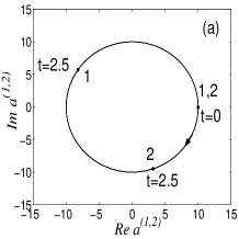
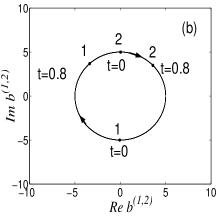
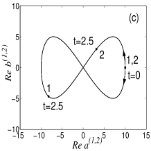
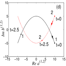
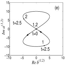
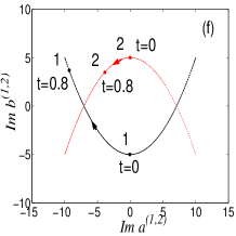
Figure 1: Phase-diagrams of the coexisting solutions (5)–(6) and (7)– (8) in black and red, respectively. The parameters are: $\mathit{Re}\,\alpha=10$, $\mathit{Im}\,\alpha=0$, $\omega=1$ and $\epsilon=0.1$. The positions of the phase points 1 and 2 are marked at the initial time $t=0$ and at the later times $t=0.8$ or $t=2.5$.

Generally, if we start from any point lying on a periodic trajectory of the system (3)– (4) we always remain in the same trajectory. This is frequently called the translation properties of autonomous systems which means that to a given trajectory corresponds an infinity of motions (solutions) differing from each other by the phase [17]. The question is, however the type of trajectories of the system (3) – (4) when the initial conditions do not lie on periodic orbits. There is no difficulty in solving this problem numerically in contradistinction to a general analytical approach. The numerical analysis shows that all trajectories of the system (3) – (4) originating from independent initial conditions $a(0)=\alpha$ and $b(0)=\beta$ (contrary to the dependent conditions $a^{(1,2)}(0)=\alpha$ and $b^{(1,2)}(0)=\pm\frac{i}{2}\sqrt{\frac{\alpha^{3}}{\alpha^{*}}}$ generating periodic orbits) behave in a nonperiodic, mainly quasiperiodc manner. For example, when $a(0)=\alpha$ and $b(0)=0$ we get an analytical result known since the pioneering work by Bloembergen [14, 15]:

$$a(t) = \alpha\,sech\left(\frac{\sqrt{2}}{2}\alpha\epsilon t\right)e^{-i\omega t}$$ (9)

$$b(t)=-\frac{\alpha}{\sqrt{2}}\tanh\left(\frac{\sqrt{2}}{2}\alpha\epsilon t\right)e^{-i2\omega t}$$ (10)

where $\alpha=\alpha^{*}$. Obviously, due to the time dependent amplitudes $\alpha\,sech\left(\frac{\sqrt{2}}{2}\alpha\epsilon t\right)$ and $-\frac{\alpha}{\sqrt{2}}\tanh\left(\frac{\sqrt{2}}{2}\alpha\epsilon t\right)$ the functions $a(t)$ and $b(t)$ are not formally periodic i.e. $a(t+T)\neq a(t)$ and $b(t+2T)\neq b(t)$, where $T=\omega/2\pi$. The solutions are frequently referred to as nearly periodic, which mearly means that in the course of time both functions approach a purely periodic motion.
Another question is the change in the harmonic solutions (5)–(8) on inclusion of damping in the dynamical system (3)–(4):

$$\frac{da}{dt} = -i\omega a-\gamma a+\epsilon a^{*}b\,,$$ (11)

$$\frac{db}{dt} = -i2\omega b-\gamma b-\frac{1}{2}\epsilon a^{2}\,,$$ (12)

where, for the sake of simplicity, we have put $\gamma_{1}=\gamma_{2}=\gamma$. Using the method [17] proposed by Krylov-Bogolubov (we do not present the details here) we get two coexisting nonperiodic solutions $\{a^{(1)}(t),b^{(1)}(t)\}$ and $\{a^{(2)}(t),b^{(2)}(t)\}$, namely:

$$a^{(1,2)}(t) = \alpha e^{-\gamma t}e^{-i[\omega t\pm\frac{\epsilon}{2\gamma}\sqrt{\alpha^{*}\alpha}(1-e^{-\gamma t})]}\,,$$ (13)

$$b^{(1,2)}(t) = \mp\frac{i}{2}\sqrt{\frac{\alpha^{3}}{\alpha^{*}}}e^{-\gamma t}e^{-i2[\omega t\pm\frac{\epsilon}{2\gamma}\sqrt{\alpha^{*}\alpha}(1-e^{-\gamma t})]}\,.$$ (14)

In the limit $\gamma\rightarrow 0$, the above functions become periodic solution (5)–(8). Here, in contradistinction to the periodic solutions, not only the amplitudes are functions of the damping constant $\gamma$ but also the phases. For $t\rightarrow\infty$ the coexisting solutions $\{a^{(1)}(t),b^{(1)}(t)\}$ as well as $\{a^{(2)}(t),b^{(2)}(t)\}$ tend to zero.
Damping damages degeneration of the periodic orbit in Fig.1 (a,b,c and e). By way of example, it is illustrated in Fig.2.

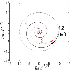
Figure 2: Phase diagram of the function (13) for $\gamma=0$ (circle) and $\gamma=0.2$ (spirals). The circle is identical to that in Fig.1a. The phase points $1$ and $2$ escape from the joint coexisting orbit due to damping. The first (black) goes faster then the second (red).

For $\gamma\neq 0$ the phase points 1 and 2, drawing different trajectories ($1$ goes faster than $2$), approach the fixed point $(0,0)$, being an attractor.
Equations (11)–(12) may be solved subject to the initial conditions $a(0)=\alpha$ and $b(0)=0$ to yield

$$a(t) = \alpha e^{-\gamma t}\,sech\left(\frac{\sqrt{2}}{2\gamma}\alpha\epsilon(1-e^{-\gamma t})\right)e^{-i\omega t}\,$$ (15)

$$b(t) = -\frac{\alpha e^{-\gamma t}}{\sqrt{2}}\tanh\left(\frac{\sqrt{2}}{2\gamma}\alpha\epsilon(1-e^{-\gamma t})\right)e^{-i2\omega t}\,.$$ (16)

The behavior of the above amplitudes and phases is remarkably different from that presented by Eqs.(13)–(14). Here, the phases depend neither on the initial conditions nor on the damping constant. The amplitudes are damped in a much more intricate way than those in Eqs. (13)–(14) .
In the phase space, both functions (13)–(14) and (15)–(16) tend to the same attractor being a fixed point. Obviously, in the limit $\gamma\rightarrow 0$ the functions (15)–(16) approach arbitrarily closely functions (9)–(10), respectively. Generally, the numerical studies show clearly that in the phase space the system (11)–(12) always tends to a fixed point, independently of the initial conditions.

2.2 Periodic resonance solutions of nonautonomous system

In order to find a periodic resonance solution of the system(1)– (2) we look for a solution in the form

$$a(t)=Xe^{-i\Omega_{1}t}\,\,,\,\,\,\,b(t)=Ye^{-i\Omega_{2}t}\,,$$ (17)

where $\Omega_{1}=\omega$ and $\Omega_{2}=2\omega$ are the resonance conditions. The amplitudes $X$ and $Y$ are constant in time. On inserting (17) into (1)– (2) we get two algebraic equations (quadratic) in the complex variables

$$-\gamma_{1}X+\epsilon X^{*}Y+F_{1}=0\,,$$ (18)

$$-\gamma_{2}Y-\frac{1}{2}\epsilon X^{2}+F_{2}=0\,.$$ (19)

Therefore, we look for $X$ and $Y$ as functions of the parameters: $\epsilon$, $\gamma_{1}$, $\gamma_{2}$, $F_{1}$ and $F_{2}$. Restricting the number of the parameter to three, we get solutions whose physical context is clear, and the algebraic form is easy for numerical investigation.

2.2.1 The case I,  $F_{1}=0$ , $F_{2}\neq 0$ , $\gamma_{1}\neq 0$ and $\gamma_{2}\neq 0$

This case ($F_{1}=0$) describes the subharmonic generation. There are two coexisting solutions $\{a^{(1)}(t),b(t)\}$ and $\{a^{(2)}(t),b(t)\}$

$$a^{(1,2)}(t) = \mp\sqrt{\frac{2F_{2}}{\epsilon}-\frac{2\gamma_{1}\gamma_{2}}{\epsilon^{2}}}\,e^{-i\omega t}\,\,\,\,,F_{2}>\frac{\gamma_{1}\gamma_{2}}{\epsilon}\,,$$ (20)

$$b(t) = \frac{\gamma_{1}}{\epsilon}e^{-i2\omega t}\,.$$ (21)

which differ only in the phase $a^{(2)}(t)=a^{(1)}(t)e^{-i\pi}$. Therefore, the coexistence has a trivial character. (see Eqs.(3.1, second line) in Ref.[10]).

2.2.2 The case II,  $F_{1}\neq 0$ , $F_{2}=0$, $\gamma_{1}\neq 0$ and $\gamma_{2}\neq 0$

Physically, this case ($F_{2}=0$) corresponds to the second harmonic generation. There are no coexisting solutions but only one single solution (see Eqs.(3) and (4) in Ref.[11]):

$$a(t) = (A+B)e^{-i\omega t}\,,$$ (22)

$$b(t) = -\frac{\epsilon}{2\gamma_{2}}(A+B)^{2}e^{-i2\omega t}\,,$$ (23)

$$A = \sqrt[3]{\frac{\gamma_{2}F_{1}}{\epsilon^{2}}+\sqrt{\left(\frac{2\gamma_{1}\gamma_{2}}{3\epsilon^{2}}\right)^{3}+\left(\frac{\gamma_{2}F_{1}}{\epsilon^{2}}\right)^{2}}}\,,$$

$$B = \sqrt[3]{\frac{\gamma_{2}F_{1}}{\epsilon^{2}}-\sqrt{\left(\frac{2\gamma_{1}\gamma_{2}}{3\epsilon^{2}}\right)^{3}+\left(\frac{\gamma_{2}F_{1}}{\epsilon^{2}}\right)^{2}}}\,.$$

2.2.3 The case III,  $F_{1}\neq 0$ , $F_{2}\neq 0$, $\gamma_{1}\neq 0$ and $\gamma_{2}=0$

Here, both the subharmonic effect and the second harmonic processes compete with each other. The assumption $\gamma_{2}=0$ describes the so-called good frequency conversion limit for subharmonic generation. It is easy to prove that the system (1)–(2) has two coexisting solutions $\{a^{(1)}(t),b^{(1)}(t)\}$ and $\{a^{(2)}(t),b^{(2)}(t)\}$ given by

$$a^{(1,2)}(t) = \mp\sqrt{\frac{2F_{2}}{\epsilon}}e^{-i\omega t}\,,$$ (24)

$$b^{(1,2)}(t) = \left(\frac{\gamma_{1}}{\epsilon}\pm\frac{F_{1}}{2F_{2}}\sqrt{\frac{2F_{2}}{\epsilon}}\,\right)e^{-i2\omega t}\,.$$ (25)

Physically, for the same values of parameters the system has two periodic states differing in the vales of amplitude. If $\frac{\gamma_{1}}{\epsilon}=\frac{F_{1}}{2F_{2}}\sqrt{\frac{2F_{2}}{\epsilon}}$, then second-harmonic vibrations are quenched ($b^{(2)}(t)=0$). In this case the subharmonic generation is maximal.

Phase diagrams for the coexisting solutions $\{a^{(1)}(t),b^{(1)}(t)\}$ and $\{a^{(2)}(t),b^{(2)}(t)\}$ are presented in Fig.(3). As seen, only the phase curve for the pair $(Re\,a^{(1)}(t),Im\,a^{(1)}(t))$ covers the phase curve for the pair $(Re\,a^{(2)}(t),Im\,a^{(2)}(t))$. Here, point $1$ is by $\pi$ out of phase with point $2$. The other curves are non-degenerate that is they are separable. This behaviour follows from the fact that the functions $b^{(1,2)}(t)$ differ in the values of amplitudes.
There is no geometrical correspondence between the phase portraits in Fig.1 and Fig.3.
The main difference is, however, between the autonomous and nonautonomous phase dynamics. The translation properties of autonomous systems ( sometimes called free phase [18]) do not hold in nonautonomous systems. It means, for example that the phase points $1$ and $2$ in Fig.3 (a) follow the circle provided that they start only from the points $(a(0)=-10$, $b(0)=0)$ and $(a(0)=+10$, $b(0)=0)$, respectively. If they start from the other points lying on the circle they escape from it, which does not take place in the autonomous case (this problem is considered in detail in Section III).
As seen from Eqs. (24)–(25) the parameter $\epsilon$ governing the nonlinearity of the system (1)–(2) is felt in the amplitudes, in contradistinction to the autonomous case, where $\epsilon$ is felt in the phases (see Eqs.(13)–(14)).

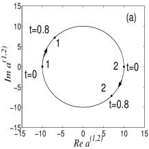
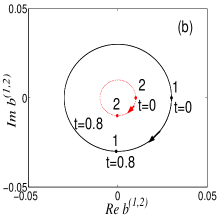
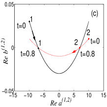
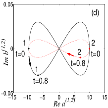
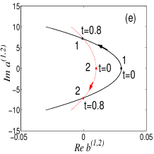
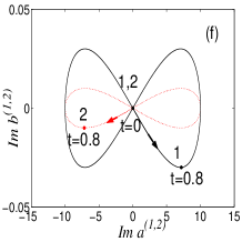
Figure 3: Phase-diagrams of the coexisting solutions (24)–(25) for $\omega=1$, $\epsilon=0.1$, $\gamma_{1}=0.002$, $F_{1}=0.01$ and $F_{2}=5$.

2.3 Fractional resonance

It is assumed that the difference between the periodic solutions of the autonomous and the nonautonomous system is mainly that the solution of the former has the period (frequency) being a function of the initial conditions and the parameter governing the nonlinearity of the system itself (vide Eqs.(5)–(8)), whereas that of the latter have period of the external pump fields only (vide Eqs. (24)–(25)).The main difference between the periodic solutions of the autonomous and nonautonomous systems is that the period of the former is a function of initial conditions and the parameter governing the nonlinearity of the system (vide Eqs.(5)–(8)), while that of the latter is determined by the external pump fields only (vide Eqs. (24)–(25)). However, in some cases the periodic solution of the nonautonomous system may have the period dependent also on the parameter governing the nonlinearity of the differential equation. This takes place in a special case of the resonance, namely when we want a nonautonomous system to vibrate at the frequency of its autonomous counterpart. Then, instead of looking for the solutions of (1)–(2) in the form of (17) we search for solutions given by (see Eqs.(5)–(8))

$$a(t)=xe^{-i\Omega_{1}t}\,,\,\,\,\,b(t)=\mp\frac{i}{2}\sqrt{\frac{x^{3}}{x^{*}}}e^{-i2\Omega_{1}t}\,,$$ (26)

where $\Omega_{1}=\omega\pm\frac{1}{2}\epsilon\sqrt{x^{*}x}$. It is easy to note that the functions (26) satisfy Eqs.(1)– (2) provided that $\gamma_{2}=0$, $F_{2}=0$ and $x=F_{1}/\gamma_{1}$. In this way the frequency $\Omega_{1}$ becomes additionally a function of the damping constant $\gamma_{1}$ and the amplitude $F_{1}$. By way of example, for $\gamma_{2}=0$, $F_{2}=0$, $\omega=1$, $\epsilon=0.1$ and $F_{1}=5$ the system (1)– (2) has a periodic solution provided that $\Omega_{1}=1\pm\frac{1}{2}$. Therefore, we have two sets equations. The first

$$\frac{da}{dt} = -ia-0.5a+0.1a^{*}b+5e^{-i\frac{3}{2}t}\,,$$ (27)

$$\frac{db}{dt} = -i2b-0.5\epsilon a^{2}\,,$$ (28)

where the solutions are given by $a(t)=10\exp(-i\frac{3}{2}t)$ and $b(t)=-5i\exp(-3it)$ and, the second

$$\frac{da}{dt} = -ia-0.5a+0.1a^{*}b+5e^{-i\frac{1}{2}t}\,,$$ (29)

$$\frac{db}{dt} = -i2b-0.5\epsilon a^{2}\,,$$ (30)

where $a(t)=10\exp(-i\frac{1}{2}t)$ and $b(t)=5i\exp(-it)$. Both sets of equations describe the so-called fractional (subharmonics, demultiplication) resonances. The periodic solutions of (27)–(28) and (29)–(30) satisfy the conservative autonomous system $da/dt=-ia+0.1a^{*}b$ and $db/dt=-i2b-0.5a^{2}$ and have phase representation identical to that in Fig.(1). Finally let us note that the system (1)–(2) if $\gamma_{2}=0$, $F_{2}=0$ and the resonance condition $\Omega_{1}=\omega$ holds, has a Bloembergen-type solution in the form:

$$a(t) = \frac{F_{1}}{\gamma_{1}}\,sech\left(\frac{\sqrt{2}}{2}\frac{F_{1}}{\gamma_{1}}\epsilon t\right)e^{-i\omega t}\,,$$ (31)

$$b(t)=-\frac{F_{1}}{\gamma_{1}\sqrt{2}}\tanh\left(\frac{\sqrt{2}}{2}\frac{F_{1}}{\gamma_{1}}\epsilon t\right)e^{-i2\omega t}\,.$$ (32)

The above functions for $t\rightarrow\infty$ tend to periodic states.

3 Chaotic behaviour

The coexisting periodic solutions (24)–(25) naturally lead to the question about the effects of a disturbance of the resonance conditions. It is intuitively clear that this problem can only be solved numerically. As a background to numerical investigations we use the equations

$$\frac{da}{dt} = -ia-0.002a+0.1a^{*}b+0.01e^{-i\Omega_{1}t}\,,$$ (33)

$$\frac{db}{dt} = -i2b-0.05a^{2}+5e^{-i\Omega_{2}t}\,,$$ (34)

where $\Omega_{1}$ and $\Omega_{2}$ play a role of parameters. If at the time $t=0$ the state of the above system is determined by the initial conditions $a(0)=10$ and $b(0)=0.01$ and the conditions of resonance are satisfied i.e. $\Omega_{1}=1$ and $\Omega_{2}=2$, then the pair of periodic functions

$$a(t)=10e^{-it}\,,\,\,\,\,\,b(t)=0.01e^{-i2t}.$$ (35)

satisfy the differential equations (33)–(34). Phase diagrams of the functions (35) are given in Fig.3 (black lines). For the initial conditions $a(0)=-10$ and $b(0)=0.03$ we get the second pair of coexisting periodic solutions (red line in Fig.3)

$$a(t)=-10e^{-it}\,,\,\,\,\,b(t)=0.03e^{-i2t}$$ (36)

Let us now consider the behaviour of the system in the neighbourhood of the resonance periodic solutions in the range

$$\Omega_{1}=1\,\,\,\,\mbox{and}\,\,\,\,0<\Omega_{2}<4\,.$$ (37)

Numerically, we solve Eqs. (33)–(34), with the help of a fourth-order Runge-Kutta method, with the initial conditions $(a(0)=10$, $b(0)=0.01)$, for $\Omega_{1}=1$ and selected values of $\Omega_{2}\neq 2$. Then, we repeat the same procedure with the initial conditions $(a(0)=10$, $b(0)=0.03)$. The numerical results are reflected in phase portraits and in the spectra of Lyapunov exponents, computed by the Wolf procedure [19].

At the beginning, let us consider two the most typical types of behaviour being a result of detuning, that is the resonance condition breaking.

Example I - large frequency detuning.
Take the frequency $\Omega_{2}=0.472$ instead of $\Omega_{2}=2$. We observe that initially the phase point follows the periodic solution (35) and then escapes from it to a chaotic state. This result of the large detuning is seen in the phase $(\mathit{Im}\,a\,,\mathit{Re}\,a)$ plane Fig.4(a). A symmetric behaviour is observed in the same phase portrait, if the system (33)–(34) starts with the initial conditions $a(0)=-10$ and $b(0)=0.03$, see Fig.4(b). The periodic ($\Omega_{2}=2$) and chaotic ($\Omega_{2}=0.472$) states of the system presented in Fig.4 confirm the spectra of the Lyapunov exponents$\{-0.0007,-0.0007,-0.0022,-0.0022\}$ and $\{0.1659,0.0012,-0.0029,-0.1699\}$, respectively. The latter spectrum, containing two positive exponents, indicates a strong chaotic behaviour, the so-called hyperchaos.

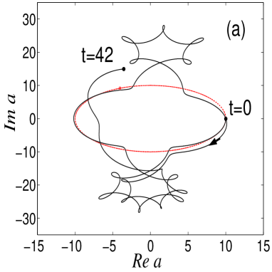
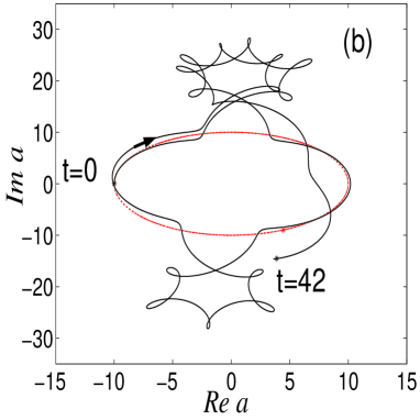
Figure 4: The symmetric escape of the phase points from the coexisting orbits. Figure (a) - evolution of the system (33)–(34) with the initial conditions $a(0)=10$, $b(0)=0.01$ and for 1) $\Omega_{1}=1$, $\Omega_{2}=2$ (periodic solution - read) and 2) $\Omega_{1}=1$, $\Omega_{2}=0.472$ (chaos - black). Figure (b)- the same as in Figure(a) but with the initial conditions $a(0)=-10$ and $b(0)=0.03$.

Example II - weak frequency detuning
Take now the frequency $\Omega_{2}=2.25$ instead of $\Omega_{2}=2$. Here, the point escapes from the periodic state (governed by Eqs.(35))to another periodic state characterized by the spectrum $\{-0.0013,-0.0014,-0.0015,-0.0015\}$. This is shown in (Fig.5). The same phase structure is obtained if the system starts from the coexisting periodic states described by Eqs.(36)).

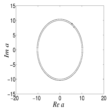
Figure 5: Escape from one periodic state (red) to another periodic state (black). Evolution of the system (33)–(34) with the initial conditions $a(0)=10$ and $b(0)=0.01$ and for 1) $\Omega_{1}=1$, $\Omega_{2}=2$ (red) and 2) $\Omega_{1}=1$, $\Omega_{2}=2.25$ (black). Black orbit has been drawn for $t>4500$, to omit the transient effects).

Globally, the behaviour of the system in the resonance neighbourhood (37) is presented in Fig.6. The spectra of the Lyapunov exponents $\{\lambda_{1},\lambda_{2},\lambda_{3},\lambda_{4}\}$ versus $\Omega_{2}$ show the regions of order or chaos. If $\lambda_{1}>0$ then system is chaotic (black colour), if simultaneously $\lambda_{1}>0$ and $\lambda_{2}>0$ then system is hyperchaotic (black and green) and finally if $\lambda_{1}\leq 0$ the system behaves nonchaotically (periodically). For $\Omega_{2}=2$ the system is in a periodic state (Eqs.(35) or solid lines in Fig.3).
Fig. (6) shows that the spectra are nearly symmetric relative to the resonance frequency $\Omega_{2}=2$. By way of example, for $\Omega_{2}=2.25$ (see Fig.5) we have the same spectrum as for $\Omega_{2}=1.75$ and get two identical phase structures.

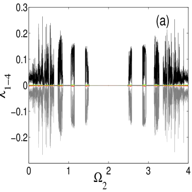
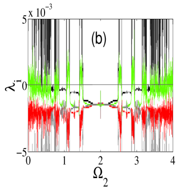
Figure 6: (a) Spectrum of Lyapunov exponents $\lambda_{i}$, $i=1,2,3,4$, for the system (33)–(34) with the initial conditions $a(0)=10$ and $b(0)=0.01$, for $\Omega_{1}=1$, and $0<\Omega_{2}<4$. (b) An enlargement of the region of $\mid\lambda_{j}\mid<5\times 10^{-3}$.

A convenient way of finding out what may be expected in the system (33)–(34) under conditions $\Omega_{1}\neq 1$ and $\Omega_{2}\neq 2$ is to calculate the maximal Lyapunow exponent $\lambda_{1}$ as a function of $\Omega_{1}$ and $\Omega_{2}$. Then, the global dynamics of the system is simply presented by the Lyapunov map in the space of ($\Omega_{1},\Omega_{2}$) (Fig.7), where the values of $\lambda_{1}$ are marked by an appropriate colour. A band structure of the map shows that the system is much more sensitive to the changes in $\Omega_{2}$ than to those in $\Omega_{1}$. This is caused by the fact that the amplitude of the forcing term in (33) is $500$ times lower than in the forcing term in (34). Therefore, the changes in $\Omega_{1}$ do not affect so much the stability of the system as those in $\Omega_{2}$. The map is simply symmetric to the line $\Omega_{1}=1$ which means that the detuning $\Omega_{2}\ +\delta$ as well as $\Omega_{2}\ -\delta$ causes the same kind of stability (instability) of the system. The cental point of the map $(\Omega_{1}=1,\Omega_{2}=2)$ corresponds to the periodic solution (35).
We might expect that if the nonlinear interaction is sufficiently weak, that is when $\epsilon/\omega<<1$, then in the presence of detuning (that is in the neighbourhood of the periodic solution (35)) beats could appear. Though the nonlinear interaction in (33)–(34) can really be treated as weak $(\omega=1,\epsilon=0.1)$ it is not sufficiently weak to induce quasiperiodic phenomenon. Distinct beats appear in (33)–(34) when $\epsilon/\omega<0.01$. This condition is satisfied (with a wide margin) if we put in (33)–(34), for example: $\Omega_{1}=\omega=100$ (instead of $\omega=1$) and $\Omega_{2}=200\pm\delta$, where $\delta$ is the value of detuning (for $\delta=0$ the system has the periodic solutions redefined $a(t)=10e^{-i100t}$ and $b(t)=0.01e^{-i200t}$). A typical example of beats is presented in Fig.8.

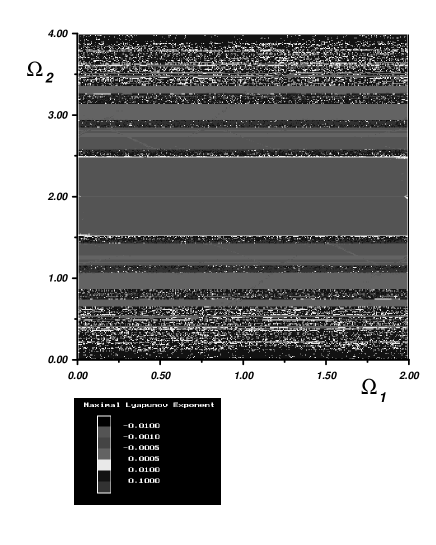
Figure 7: The values of maximal Lyapunov exponents for Eqs.(33)–(34) with the conditions $a(0)=10$ and $b(0)=0.01$ if $0<\Omega<2$ and $0<\Omega_{2}<4$.

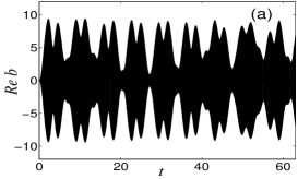
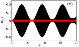
Figure 8: Beats. Time evolution $\mathit{Re}\,b(t)$ of the system (1)-(2) where $\omega=100$, $\gamma_{1}=0.002$, $\gamma_{2}=0$, $F_{1}=0.01$, $F_{2}=5$, $\Omega_{1}=100$ and the initial conditions are $a(0)=10$ and $b(0)=0.01$ and for (a) $\Omega_{2}=202$, (b) $\Omega_{2}=200.1$. The red band in (b) represents the periodic solution $\Omega_{2}=200$.

The beats proceed as follows: if $\Omega_{2}$ tends to $2\omega=200$ i.e. ($\delta\rightarrow 0$) the amplitude of beats increases but this happens only to a certain value of the difference $|2\omega-\Omega_{2}|=\Delta$ (in our case $\Delta=0.5$) after which the amplitude of beats began to decrease. Finally beats disappear for $2\omega=\Omega_{2}=200$ that is in the resonance. The beats problem (also chaotic beats) in different nonlinear systems has been recently investigated in nonlinear optics [20] and in electric circuits [21].

Nonautonomous systems do not manifest the so-called translation properties as their autonomous counterparts do. This property can be readily reflected in phase portraits. By way of example, to demonstrate this behaviour we use Fig.3a (black). If the system (33)– (34) starts from the point $A=(a(0)=10,b(0)=0.01)$ then in the phase portrait we observe a circle (the periodic solution (35)). However, if the same system starts from another point $B\neq A$, lying on the circle, it does not remain on the circle but escapes from it and draws another curve - in our case of chaotic one (Fig.9). This chaotic behaviour is confirmed by the spectrum of the Lyapunov exponents $\{0.0059,-0.0009,-0.0031,-0.0077\}$.
Generally, the system can escape from the periodic orbit to stable (periodic) states or to chaotic states. On calculating the maximal Lyapunov exponents $\lambda_{1}$ for the system starting from individual points of the periodic orbit we get the information on which orbit is chaotic $\lambda_{1}>0$ and which is nonchaotic $\lambda_{1}\leq 0$. This is shown in Fig.(10).

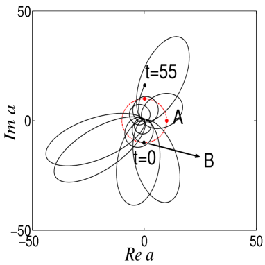
Figure 9: Escape of the phase curve starting from the point $B$ lying on the periodic curve (red circle). The periodic orbit, generated the system (33)–(34), starts from the point $A$ (the initial conditions: $a(0)=10$ and $b(0)=0.01$). The same system on starting from $B$ (the initial condition) $a(0)=-0.0922-i10.0196$ and $b(0)=0.0102-i0.002$ behaves chaotically.

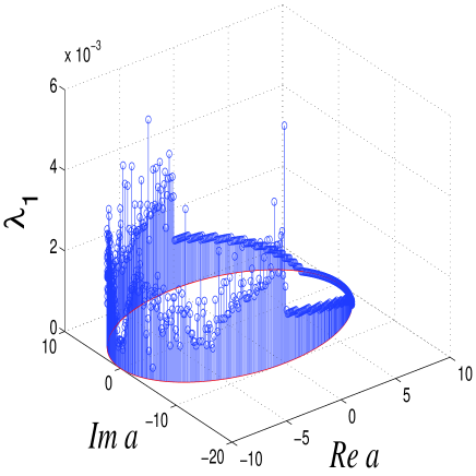
Figure 10: Maximal Lyapunov exponents $\lambda_{1}\geq 0$ for the trajectories of system (33)–(34) started from different points of the periodic orbit (red) in Fig.9. The individual values of $\lambda_{1}$ show from which points (lying on the orbit) chaotic ($\lambda_{1}>0$) , and from which nonchaotic ($\lambda_{1}=0$) phase curves originate.

4 Synchronization of the coexisting states.
Quenching

Let us now consider the synchronization problem (mutual or unidirectional) of two dynamical systems $(a,b)$ and $(A,B)$, which we may assume to be identical in all respects but being in two coexisting periodic states. We take the system $(a,b)$ given by (1) – (2) and its copy $(A,B)$ and couple them linearly:

$$\frac{da}{dt} = -i\omega a-\gamma_{1}a+\epsilon a^{*}b+F_{1}e^{-i\Omega_{1}t}$$

$$- S_{(a,A)}(a-A)\,,$$

$$\frac{db}{dt} = -i2\omega b-\gamma_{2}b-\frac{1}{2}\epsilon a^{2}+F_{2}e^{-i\Omega_{2}t}$$

$$- S_{(b,B)}(b-B)\,$$

$$\frac{dA}{dt} = -i\omega A-\gamma_{1}A+\epsilon A^{*}B+F_{1}e^{-i\Omega_{1}t}$$

$$- S_{(A,a)}(A-a)\,$$

$$\frac{dB}{dt} = -i2\omega B-\gamma_{2}B-\frac{1}{2}\epsilon A^{2}+F_{2}e^{-i\Omega_{2}t}\,$$

$$- S_{(B,b)}(B-b)\,$$

where $S_{(i,j)}=S_{(j,i)}$ is a parameter of the coupling. The coupling is usually turned on at an arbitrarily chosen time.
The most spectacular behaviour is observed if the systems $(a,b)$ and $(A,B)$ are autonomous and conservative, that is when $\gamma_{1}=\gamma_{2}=0$ and $F_{1}=F_{2}=0$. Suppose that the system $(a,b)$ is in the state (5) – (6) whereas $(A,B)$ is in the state (7) – (8). This means that the oscillator $a$ vibrates at the frequency $\omega+\delta$, where $\delta=0.5\epsilon\sqrt{\alpha^{*}\alpha}$, whereas the oscillator $A$ vibrates at the frequency $\omega-\delta$. The oscillators $b$ and $B$ vibrate at the frequencies $2(\omega+\delta)$, $2(\omega-\delta)$, respectively. Therefore, the pairs$(a,b)$ and $(A,B)$ are simply detuned in frequencies. If the oscillator pairs $(a,b)$ and $(A,B)$ are mutually coupled, they get synchronized. This is illustrated in Fig.11.

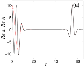
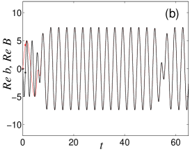
Figure 11: The temporal oscillation death in $a,A$-components, black and red, respectively (a); and oscillation in $b,B$-components (b). The effect forced by mutual synchronization in the system (4)–(4) with the initial conditions $a(0)=10$, $b(0)=5$, $A(0)=10$, $B(0)=-5$, for $\omega=1$, $\epsilon=0.1$, $\gamma_{1}=\gamma_{2}=0$, $F_{1}=F_{2}=0$ and $S_{a,A}=S_{b,B}=S_{A,a}=S_{B,b}=0.5$. The $S$-terms are turned at $t=10$.

As seen, the coupling $S=0.5$ is turned on at $t=10$ and the systems synchronize at $t=15$. Consequently, for $t>15$ $a(t)=A(t)$ and $b(t)=B(t)$. What is more, the oscillator $a$ and $A$ are quenched for some time but at the same time the oscillators $b$ and $B$ vibrate periodically with the double frequency $2\omega$. As seen from Fig.11 after the oscillation death in $a,A$-components we always observe its rapid and short revival – these effects occur one after the other. The revivals always correspond to appropriate collapses in $b,B$-components The quenching interval depends on the coupling constant $S$, the lager the value of $S$ the longer the quenching interval. Therefore, the quenching effect is the most effective in the case of strong interaction that is when $S>>\omega$. The quenching phenomenon is forced by the real parts of the $S_{i,j}$-terms in 4-4. They are simply the momentum (velocity) terms, sometimes named diffusive [22], being sources of dissipation in the individual systems.

Complete quenching can be obtained in the case of unidirectional interaction. Suppose, that $S_{(B,b)}=S_{(A,a)}=0$, which means that $(A,B)$ is a transmitter (master) system and $(a,b)$ is a receiver (slave) system. Moreover, the transmitter sends a continuous signal [23] that it is in the state described by (7) – (8) because we choose the frequency $\omega=\frac{1}{2}\epsilon\sqrt{\alpha^{*}\alpha}$. It is possible, for example, if $\omega=0.5$, $\alpha=10$, $S_{a,A}=S_{b,B}=0.5$ and $\epsilon=0.1$ (Fig.12). Physically, it means that the transmitter does not vibrate. The receiver is in a periodic state (5) – (6). On turning on the coupling the vibrations in the receiver are quenched – oscillation death is complete. The total quenching can be spectacularly observed with the help of the phase plots in Fig.1 (a). Namely, the phase point $2$ does not move, whereas point $1$ follows the periodic orbit. At the moment we turn on the synchronization mechanism and point $1$ moves slower and slower towards point $2$, and finally approaches the point $2$ – the orbit is quenched. A similar behaviour is observed in Fig.1 (b), (c) and (e). In Fig.1 (d) and (f) point $2$ does not lie on the orbit of point $1$. Point $1$ moves up and down along the parabole. If we turn on the synchronization mechanism point $1$ escapes from its orbit and tends to point $2$ – the orbit is quenched. Also, the inverse process is possible, that is creation of an orbit for point $2$.

With the help of the unidirectional synchronization we can force the phase point in Fig.9 to return and escape chaotically from the periodic orbit. To do that, it is necessary to use the system(4)–(4)with $S_{(A,a)}=S_{(B,b)}=0$, $\gamma_{1}=0.002$ $,\gamma_{2}=0$, $F_{1}=0.01$, $F_{2}=5$, $\Omega_{1}=1$, $\Omega_{2}=2$ and the initial conditions $a(0)=-0.0922-i10.0196$, $b(0)=0.0102-i0.002$ (chaotic orbit) and $a(0)=10$ and $b(0)=0.01$ (red circle). Moreover, the terms $S_{(a,A)}=S_{(b,B)}=0.5$ should be turned on at $t=10$, then we observe the situation presented in Fig.13.
Synchronization of the nonautonomous coexisting states is as easy as that of the autonomous ones. The resultant vibrations usually appear as intricate revivals and collapses, frequently chaotic.

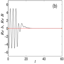
Figure 12: The complete quenching caused by unidirectional synchronization in the system(4)–(4) with the initial conditions $a(0)=10$, $b(0)=5$, $A(0)=10$, $B(0)=-5$, for $\omega=0.5$, $\epsilon=0.1$, $\gamma_{1}=\gamma_{2}=0$, $F_{1}=F_{2}=0$ and $S_{(A,a)}=S_{(B,b)}=0$. The terms $S_{(a,A)}=S_{(b,B)}=0.5$ are turned on at $t=10$.

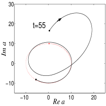
Figure 13: Return to the periodic orbit of a point chaotically escaping from it. The escape is shown in Fig.9. The return is caused by unidirectional synchronization switched at the time $t=55$.

5 Conclusions

The coexisting periodic solutions, presented and analyzed in this paper, are a natural feature of the nonlinear differential equations (1)–(2) describing nonlinear optical processes of the second order.
The coexisting solutions of the autonomous type (5)–(8) have a simple physical interpretation. Namely, we are able to prepare the initial states of two independent harmonic oscillators (of the frequencies $\omega$ and $2\omega$) in such a way that after turning on the nonlinear interaction the oscillators vibrate at the detuned frequencies $\omega+\delta$ and $2(\omega+\delta)$ or at the coexisting frequencies $\omega-\delta$ and $2(\omega-\delta)$. If the system is damped, this correction also depends on the damping constant. This is clearly seen from Eqs.(13)–(14). The coexistence in frequency but not in amplitudes seems to be characteristic of a large class of nonlinear autonomous systems in the so-called rotating wave approximation (see Appendix). Switching on a linear coupling between the two coexisting detuned systems leads to the temporal disappearance of $(\omega\pm\delta)$-vibrations and the appearance of $2\omega$-vibrations only. The quenching interval can be controlled by the coupling parameter. In special cases (unidirectional coupling) we are able to completely annihilate vibrations in both oscillators being in the coexisting states.

The physical interpretation of the coexisting solutions for the nonautonomous case is different to that presented above. The nonlinearity is now concealed in amplitude, and the frequency is a parameter of the system. Two periodic solutions, having the same resonance frequency, have different amplitudes (or the same amplitudes but different signs). Therefore, the coexistence means here a possibility of existence of two resonance states at the same values of parameters. The structure of the coexisting states in the phase space is completely degenerate as in the case of Eqs. (20)–(21). The difference is only in phase, or partially degenerate as in the case of solutions (24)–(25). In the latter case, it means that in some subspace (Fig.3(a)) two different coexisting states have identical phase curves. Changing the external parameters of the system, for example the external pump frequency, we can control the phase structure of the coexisting states. Consequently we can make the system jump from a coexisting state to a periodic, quasiperiodic (beats) or chaotic state.

6 Appendix

The method presented is a version of the Lindstedt’s method [17](p.224), applied to autonomous systems in complex variables. If this method is applied to differential eqations of nonlinear optics written in the rotating wave approximation it gives the so-called closed solution. Otherwise, we get series solutions. Below we show how this method works for the system(3)–(4). Moreover, we present other periodic solutions of the selected equations of nonlinear optics.

6.1 Second-harmonic problem

We find a periodic solution of Eqs.(3)–(4). The problem is considered for arbitrary initial conditions: $a(0)=\alpha$ and $b(0)=\beta$. It is obvious that if $\epsilon=0$ the system(3)–(4) has a periodic solution given by the functions : $a(t)=\alpha\exp{(-i\omega t)}$ and $b(t)=\beta\exp{(-i2\omega t)}$. Now, we suppose that if $\epsilon\neq 0$ the set of equations (3)–(4) also has periodic solution with unknown frequencies $\Omega$ and $2\Omega$. In order to avoid dealing with the unknown frequencies in the system (3)–(4) we put $\Omega t=\omega\tau\,$. This leads to

$$a(t)=a\left(\frac{\omega\tau}{\Omega}\right)=A(\tau)\,,\,\,\,\,\,b(t)=b\left(\frac{\omega\tau}{\Omega}\right)=B(\tau)\,,$$ (42)

and

$$\frac{da}{dt}=\frac{dA}{d\tau}\frac{\Omega}{\omega}\,,\,\,\,\,\,\frac{db}{dt}=\frac{dB}{d\tau}\frac{\Omega}{\omega}\,.$$ (43)

On inserting (42) and (43) into (3)–(4) we obtain the equations of motion in the new variables:

$$\frac{\Omega}{\omega}\frac{dA}{d\tau} = -i\omega A+\epsilon A^{*}B\,,$$

$$\frac{\Omega}{\omega}\frac{dB}{d\tau} = -i2\omega B-0.5\epsilon A^{2}\,.$$ (44)

In this case we can look for series solutions of the form:

$$A = A_{0}+\epsilon A_{1}+\epsilon^{2}A_{2}+...$$ (45)

$$B = B_{0}+\epsilon B_{1}+\epsilon^{2}B_{2}+...$$ (46)

$$\Omega = \omega+\epsilon\omega_{1}+\epsilon^{2}\omega_{2}+...$$ (47)

On substituting (45), (46) and (47) into(6.1) we get a recursive set of equations:

$$\dot{A}_{0} = -i\omega A_{0}\,,$$ (48)

$$\dot{B}_{0} = -i2\omega B_{0\,,}$$ (49)

$$\dot{A}_{1} = -i\omega A_{1}-\frac{\omega_{1}}{\omega}\dot{A}_{0}+A^{*}_{0}B_{0}\,,$$ (50)

$$\dot{B}_{1} = -2i\omega B_{1}-\frac{\omega_{1}}{\omega}\dot{B}_{0}-0.5A^{2}_{0}\,,$$ (51)

$$\dot{A}_{2} = -i\omega A_{2}-\frac{\omega_{1}}{\omega}\dot{A}_{1}-\frac{\omega_{2}}{\omega}\dot{A}_{0}+A_{1}^{*}B_{0}+A_{0}^{*}B_{1}\,,$$ (52)

$$\dot{B}_{2} = -i2\omega B_{2}-\frac{\omega_{1}}{\omega}\dot{B}_{1}-\frac{\omega_{2}}{\omega}\dot{B}_{0}-A_{0}A_{1}\,,$$

$$..........................................................$$

with the initial conditions:

$$A_{0}(0)=\alpha\,,\,\,\,\,\,\,\,B_{0}(0)=\beta\,,$$

$$A_{i}(0)=0\,,\,\,\,\,\,\,\,B_{i}(0)=0\,\,\,\,\,\mbox{for}\,\,\,i>0\,.$$ (54)

The dot denotes that differentiations are with respect to $\tau$. The zero-order solutions are:

$$A_{0}(\tau)=\alpha e^{-i\omega\tau}\,,$$ (55)

$$B_{0}(\tau)=\beta e^{-i2\omega\tau}\,.$$ (56)

On substituting (55) and (56) into (50) and (51) we have:

$$\dot{A}_{1} = -i\omega A_{1}+i\omega_{1}\alpha e^{-i\omega\tau}+\alpha^{*}\beta e^{-i\omega\tau}\,,$$ (57)

$$\dot{B}_{1} = -i2\omega B_{1}+i2\omega_{1}\beta e^{-2i\omega\tau}-0.5\alpha^{2}e^{-i2\omega\tau}\,.$$ (58)

The secular terms are: $i\omega_{1}\alpha e^{-i\omega\tau}+\alpha^{*}\beta e^{-i\omega\tau}$ and $i2\omega_{1}\beta e^{-i2\omega\tau}-0.5\alpha^{2}e^{-2i\omega\tau}$. To eliminate the secular terms we put

$$i\omega_{1}\alpha+\alpha^{*}\beta=0\,,$$ (59)

$$i2\omega_{1}\beta-0.5\alpha^{2}=0\,.$$ (60)

These assumptions reduce the set of equations (57) – (58) to the form

$$\dot{A}_{1} = -i\omega A_{1}\,,$$ (61)

$$\dot{B}_{1} = -i2\omega B_{1}\,.$$ (62)

The above equations with zero initial conditions $A_{1}(0)=0$ and $B_{1}(0)=0$ have trivial solutions, therefore : $A_{1}(\tau)=0$ and $B_{1}(\tau)=0$. Now, we calculate the new frequency $\Omega=\omega+\epsilon\omega_{1}$. From (59) and (60) we obtain $\omega_{1}=i\frac{\alpha^{*}\beta}{\alpha}$ and $\omega_{1}=-\frac{i}{4}\frac{\alpha^{2}}{\beta}$. This is only possible if $\beta=\pm\frac{i}{2}\sqrt{\frac{\alpha^{3}}{\alpha^{*}}}$. Therefore, we have $\Omega=\omega\pm 0.5\epsilon\sqrt{\alpha^{*}\alpha}$. Finally, from (45)–(46) and (42) we get

$$a(t) = \alpha e^{-i(\omega\pm\frac{1}{2}\epsilon\sqrt{\alpha^{*}\alpha})t}+\epsilon*0$$ (63)

$$b(t) = \mp\frac{i}{2}\sqrt{\frac{\alpha^{3}}{\alpha^{*}}}e^{-i2(\omega\pm\frac{1}{2}\epsilon\sqrt{\alpha^{*}\alpha})t}+\epsilon*0$$ (64)

Now, we can consider second-order corrections. Because $A_{1}=0$ and $B_{1}=0$, Eqs (52)–(6.1) have the form:

$$\dot{A}_{2} = -i\omega A_{2}-\frac{\omega_{2}}{\omega}\dot{A}_{0}=-i\omega A_{2}+i\omega_{2}\alpha e^{-i\omega\tau}\,,$$ (65)

$$\dot{B}_{2} = -i2\omega B_{2}-\frac{\omega_{2}}{\omega}\dot{B}_{0}=-i2\omega B_{2}+i2\omega_{2}e^{-i2\omega\tau}\,.$$ (66)

The secular terms are: $(\omega_{2}/\omega)\dot{A}_{0}$ and $(\omega_{2}/\omega)\dot{B}_{0}$. Therefore, we have to put $\omega_{2}=0$ which leads to the following equations:

$$\dot{A}_{2} = -i\omega A_{2}\,,$$ (67)

$$\dot{B}_{2} = -i2\omega B_{2}\,.$$ (68)

The above equations also have (with zero-initial conditions) zero-solutions: $A_{2}(\tau)=0$ and $B_{2}(\tau)=0$. Consequently:

$$a(t) = \alpha e^{-i(\omega\pm\frac{1}{2}\epsilon\sqrt{\alpha^{*}\alpha})t}+\epsilon*0+\epsilon^{2}*0$$ (69)

$$b(t) = \mp\frac{i}{2}\sqrt{\frac{\alpha^{3}}{\alpha^{*}}}e^{-i2(\omega\pm\frac{1}{2}\epsilon\sqrt{\alpha^{*}\alpha})t}+\epsilon*0+\epsilon^{2}*0$$ (70)

Generally, the mathematical induction method leads to $\omega_{i}=0$ and $A_{i}(\tau)=B_{i}(\tau)=0$ for $i>1$. Therefore, the above solutions are closed. Finally, we have:

$$a(t) = \alpha e^{-i(\omega\pm\epsilon\frac{1}{2}\sqrt{\alpha^{*}\alpha})t}\,,$$ (71)

$$b(t) = \mp\frac{i}{2}\sqrt{\frac{\alpha^{3}}{\alpha^{*}}}e^{-i2(\omega\pm\frac{1}{2}\epsilon\sqrt{\alpha^{*}\alpha})t}\,.$$ (72)

Remark.The first integral of the system (3)–(4) is of the form $\omega a^{*}(t)a(t)+2\omega b^{*}(t)b(t)=const$. The solutions of Eqs. (71)–(72) naturally implies that $a^{*}(t)a(t)=const$ and $b^{*}(t)b(t)=const$ (see also [16]).

6.2 Another selected solutions

The method presented also allow us to find a periodic solution if the number of equations is lager than two, for example [24]:

$$\frac{da}{dt} = -i\omega_{a}a+\epsilon cb^{*}\,,$$

$$\frac{db}{dt} = -i\omega_{b}b+\epsilon ca^{*}\,,$$

$$\frac{dc}{dt} = -i\omega_{c}c-\epsilon ab\,,$$ (73)

where $\omega_{c}=\omega_{a}+\omega_{b}$. Eqs. (6.2) are used to describe the so-called parametric optical processes [15]. If the initial conditions denoted by $a(0)=a$, $b(0)=b$ and $c(0)=c$ satisfy the relation $c=\frac{\mp iab}{\sqrt{a^{*}\alpha+b^{*}b}}$ then the periodic solution is given by

$$a(t) = ae^{-i\left(\omega_{a}\pm\epsilon\frac{b^{*}b}{\sqrt{a^{*}a+b^{*}b}}\right)t}\,,$$

$$b(t) = be^{-i\left(\omega_{b}\pm\epsilon\frac{a^{*}a}{\sqrt{a^{*}a+b^{*}b}}\right)t}\,,$$

$$c(t) = \frac{\mp iab}{\sqrt{a^{*}a+b^{*}b}}\,e^{-i\left(\omega_{c}\pm\epsilon\sqrt{a^{*}a+b^{*}b}\right)t}\,.$$ (74)

The method presented is also useful if the nonlinearities in a dynamical system are of different rank (for example, Kerr effect in the presence of second-harmonic generation [25]):

$$\frac{da}{dt} = -i\omega a+\epsilon a^{*}b-i\kappa a^{*}a^{2}\,,$$ (75)

$$\frac{db}{dt} = -i2\omega b-\frac{1}{2}\epsilon a^{2}\,.$$ (76)

We obtain:

$$a(t) = \alpha e^{-i\Omega t}\,,$$ (77)

$$b(t) = \left(i\frac{\kappa}{2\epsilon}\alpha^{2}\mp\frac{1}{2}i\sqrt{\frac{\kappa^{2}}{\epsilon^{2}}\alpha^{4}+\frac{\alpha^{3}}{\alpha^{*}}}\,\,\right)e^{-i2\Omega t}\,,$$ (78)

$$\Omega = \omega+\frac{1}{2}\left(\kappa\alpha^{*}\alpha\pm\sqrt{\kappa^{2}\alpha^{*2}\alpha^{2}+\epsilon^{2}\alpha^{*}\alpha}\,\right)\,,$$

where $\kappa=\epsilon\lambda$ ($\lambda$ is a numerical coefficient). The assumption $\kappa=\epsilon\lambda$ is necessary in the method presented. For $\lambda=0$ we get the solutions (71)-(72).

References

- [1] J. Guckenheimer and P. Holmes, Nonlinear Oscillations, Dynamical Systems, and Bifurcation of Vector Fields (Springer-Verlag, New York, 1983).
- [2] J. Curry, Commun. Math. Phys. 68, 129 (1979).
- [3] F. T. Arecchi, R. Meucci, G. Puccioni, and J. Tredicce, Phys. Rev. Lett. 49, 1217 (1982).
- [4] F.T. Arecchi and R.H. Harrison (eds), Instabilities and chaos in quantum optics, Springer-Verlag, Berlin, 1987.
- [5] E. Brun, B. Derighette, D. Meier, R. Holzner, and M. Raveni, J. Opt. Soc. Am. B 2, 156 (1985).
- [6] J. Maurer and A. Libchaber, J. Phys. (Paris) Lett. 41, 515 (1980).
- [7] J. M. T. Thompson and H. B. Stewart, Nonlinear Dynamics and Chaos (Wiley, Chichester, 1986).
- [8] A. Goldbeter and J.-L. Martiel, FEBS Lett. 191, 149 (1985); D. R. Chialvo and A. V. Apkarian, J. Stat. Phys. 70, 373 (1990).
- [9] J. Foss, A. Longtin, B. Mensour, and J. Milton, Phys. Rev. Lett. 76, 708 (1996).
- [10] P. Drummond, K. McNeil, and D. Walls, Opt. Acta 27, 321 (1980).
- [11] P. Mandel and T. Erneux, Opt. Acta 29, 7 (1982).
- [12] C. Savage and D. Walls, Opt. Acta 30, 557 (1983).
- [13] W. Gao, Phys. Lett. A 331, 292 (2004).
- [14] N. Bloembergen, Nonlinear Optics, Benjamin, 1965.
- [15] J. Perina, Quantum Statistics of Linear and Nonlinear Optical Phenomena, Kluwer Academic Publishers, Dordrecht, 1991.
- [16] G. Drobny, A. Bandilla, and I. Jex, Phys. Rev. A 55, 78 (1997).
- [17] N. Minorsky, Nonlinear Oscillations, Van Nostrand, Princeton, +1962.
- [18] A. Pikovsky, M. Rosenblum, and J. Kurths, Synchronization - a universal concept in nonlinear sciences, in Cambridge Nonlinear Sciences Series 12 , Cambridge Univ. Press 2001.
- [19] A. Wolf, J.B. Swift, H.L. Swinney and J.A. Vastano, Physica D16, 285 (1985).
- [20] K. Grygiel and P. Szlachetka, Int. J. Bifurcation and Chaos 12, 635 (2002).
- [21] D. Cafagna and G. Grassi, Int. J. Bifurcation and Chaos 15 (7), 2247 (2005).
- [22] D. G. Aronson, G. B. Ermentrout, and N. Koppel, Amplitude response of coupled oscillators, Physica D 41, 403-449 (1990).
- [23] K. Pyragas, Phys. Lett. A 170, 421 (1992).
- [24] A. Bandilla, G. Drobny, and I. Jex, Opt. Commun. 128, 353 (1996).
- [25] A. B. Klimov, L. L. Sanchez-Soto, and J. Delgado, Opt. Commun. 191, 419-426 (2001). Part 2, Ser.: Advances in Chemical Physics, Volume 119, ed. M.W.Evans , J. Wiley & Sons, 2001, p. 353-427.