Symmetry Breaking in Symmetric and Asymmetric Double-Well Potentials

Abstract

Motivated by recent experimental studies of matter-waves and optical beams in double well potentials, we study the solutions of the nonlinear Schrödinger equation in such a context. Using a Galerkin-type approach, we obtain a detailed handle on the nonlinear solution branches of the problem, starting from the corresponding linear ones and predict the relevant bifurcations of solutions for both attractive and repulsive nonlinearities. The results illustrate the nontrivial differences that arise between the steady states/bifurcations emerging in symmetric and asymmetric double wells.

Introduction. It is well known that the nonlinear Schrödinger (NLS) equation is a fundamental model describing the evolution of a complex field envelope in nonlinear dispersive media NLS . As such, it plays a key role in many different contexts, ranging from nonlinear and atom optics to plasma physics, fluid dynamics, and even biophysical models trubatch . The interest in the NLS equation has dramatically increased during the last few years, as it also describes the mean-field dynamics of Bose-Einstein condensates (BECs) gbec . In this context, the NLS is also known as the Gross-Pitaevskii (GP) equation, and typically incorporates external potentials that are used for the BEC confinement. Such potentials may be, e.g., harmonic (usually implemented by external magnetic fields) or periodic (implemented by the interference of laser beams), so-called optical lattices reviewsbec . Importantly, NLS models with similar external potentials appear also in the context of optics, where they respectively describe the evolution of an optical beam in a graded-index waveguide or in periodic waveguide arrays kivshar ; reviewsopt .

Another type of external potential, which has mainly been studied theoretically in the BEC context smerzi ; kiv2 ; mahmud ; bam ; Bergeman_2mode ; infeld is the double well potential. Moreover, it has been demonstrated experimentally that a BEC either tunnels and performs Josephson oscillations between the wells, or is subject to macroscopic quantum self-trapping markus1 . On the other hand, in the context of optics, a double well potential can be created by a two-hump self-guided laser beam in Kerr media HaeltermannPRL02 . A different alternative was offered in zhigang , wherein the first stages of the evolution of an optical beam, initially focused between the wells of a photorefractive crystal, were monitored.

One of the particularly interesting features of either matter-waves or optical beams in double well potentials is the spontaneous symmetry breaking, i.e., the localization of the respective order parameter in one of the wells of the potential. Symmetry breaking solutions of the NLS model have first been predicted in the context of molecular states ms and, apart from the physical contexts of BECs smerzi ; kiv2 ; mahmud ; bam ; Bergeman_2mode ; infeld (see also jackson ) and optics HaeltermannPRL02 ; zhigang mentioned above, they have also been studied from a mathematical point of view in Refs. mathsy ; mathsy1 .

These works underscore the relevance and timeliness of a better understanding of the dynamics of nonlinear waves in double well potentials. In view of that, in the present work we offer a systematic methodology, based on a two-mode expansion, of how to tackle problems in double wells, as regards their stationary states and the bifurcations (and ensuing instabilities) that arise in them. This way, considering both cases of attractive and repulsive nonlinearities, we illustrate the ways in which a symmetric double well potential is different from an asymmetric one. In particular, we demonstrate that, contrary to the case of symmetric potentials where symmetry breaking follows a pitchfork bifurcation, in asymmetric double wells the bifurcation is of the saddle-node type.

The paper is structured as follows: in Section II, we present the model and set the analytical framework. In Section III, we illustrate the value of the method by highlighting the significant differences of symmetric and asymmetric double wells. Finally, in Section IV, we summarize our findings and discuss future directions.

Model and Analytical Approach. In a quasi-1D setting, the evolution of the mean-field wavefunction of a BEC reviewsbec (or the envelope of an optical beam kivshar ) is described by the following normalized NLS (GP) equation,

$$iu_{t}=-\frac{1}{2}u_{xx}+s|u|^{2}u+V(x)u-\mu u.$$ (1)

In the BEC (optics) context, $\mu$ denotes the chemical potential (propagation constant) and $s=\pm 1$ for attractive or repulsive interatomic interactions (focusing or defocusing Kerr nonlinearity) respectively; below, for simplicity, we will adopt the terms attractive and repulsive nonlinearity for $s=\pm 1$ respectively. Finally, in Eq. (1), $V(x)$ is the double well potential, which is assumed to be composed by a parabolic trap (of strength $\Omega$) and a ${\rm sech}^{2}$-shaped barrier (of strength $V_{0}$, width $w$ and location $x_{0}$); in particular, $V(x)$ is of the form:

$$V(x)=\frac{1}{2}\Omega^{2}x^{2}+V_{0}{\rm sech}^{2}\left(\frac{x-x_{0}}{w}\right),$$ (2)

with the choice $x_{0}=0$ ($x_{0}\neq 0$) corresponding to a symmetric (asymmetric) double well. Note that such a double well can be implemented in BEC experiments upon, e.g., combining a magnetic trap with a sharply focused, blue-detuned laser beam expd . Similar double wells can also be implemented e.g., in optical systems.

The spectrum of the underlying linear Schrödinger equation ($s=0$) consists of a ground state, $u_{0}(x)$, and excited states, $u_{l}(x)$ ($l\geq 1$). In the nonlinear problem, using a Galerkin-type approach, we expand $u(x,t)$ as,

$$u(x,t)=c_{0}(t)u_{0}(x)+c_{1}(t)u_{1}(x)+\cdots,$$ (3)

and truncate the expansion, keeping solely the first two modes; here $c_{0,1}(t)$ are unknown time-dependent complex prefactors. It is worth noticing that such an approximation (involving the truncation of higher order modes and the spatio-temporal factorization of the wavefunction), is expected to be quite useful for a weakly nonlinear analysis. In fact, as will be seen below, we will be able to identify the nonlinear states that stem from the linear ones, as well as their bifurcations.

Substituting Eq. (3) into Eq. (1), and projecting the result to the corresponding eigenmodes, we obtain the following ordinary differential equations (ODEs):

$$i\dot{c}_{0} = (\omega_{0}-\mu)c_{0}-sA_{0}|c_{0}|^{2}c_{0}-sB(2|c_{1}|^{2}c_{0}+c_{1}^{2}\bar{c}_{0}),$$ (4)

$$- s\Gamma_{1}|c_{1}|^{2}c_{1}-s\Gamma_{0}(2|c_{0}|^{2}c_{1}+c_{0}^{2}\bar{c}_{1})$$

$$i\dot{c}_{1} = (\omega_{1}-\mu)c_{1}-sA_{1}|c_{1}|^{2}c_{1}-sB(2|c_{0}|^{2}c_{1}+c_{0}^{2}\bar{c}_{1}),$$ (5)

$$- s\Gamma_{0}|c_{0}|^{2}c_{0}-s\Gamma_{1}(2|c_{1}|^{2}c_{0}+c_{1}^{2}\bar{c}_{0}).$$

In Eqs. (4)-(5), dots denote time derivatives, overbars denote complex conjugates, $\omega_{0,1}$ are the eigenvalues corresponding to the eigenstates $u_{0,1}$, while $A_{0}=\int u_{0}^{4}dx$, $A_{1}=\int u_{1}^{4}dx$, $B=\int u_{0}^{2}u_{1}^{2}dx$, $\Gamma_{0}=\int u_{0}u_{1}^{3}dx$ and $\Gamma_{1}=\int u_{1}u_{0}^{3}dx$ are constants. Recall that $u_{0}$ and $u_{1}$ are real (due to the Hermitian nature of the underlying linear Schrödinger problem) and are also orthonormal. Notice also that in the symmetric case ($x_{0}=0$), due to the parity of the eigenfunctions, $\Gamma_{0}=\Gamma_{1}=0$.

We now use amplitude-phase (action-angle) variables, $c_{j}=\rho_{j}e^{i\phi_{j}}$, $j=0,1$ ($\rho_{j}$ and $\phi_{j}$ are assumed to be real), to derive from the ODEs (4)-(5) a set of four equations. Introducing the function $\varphi\equiv\phi_{1}-\phi_{0}$, we find that the equations for $\rho_{0}$ and $\phi_{0}$ are,

$$\dot{\rho}_{0} = s[(\Gamma_{0}\rho_{0}^{2}+\Gamma_{1}\rho_{1}^{2})\sin(\varphi)-\rho_{1}^{2}\rho_{0}\sin(2\varphi)],$$ (6)

$$\dot{\phi}_{0} = (\omega_{0}-\mu)+sA_{0}\rho_{0}^{2}+2sB\rho_{1}^{2}+sB\rho_{1}^{2}\cos(2\varphi)$$ (7)

$$+ s\left(\frac{\Gamma_{1}\rho_{1}^{3}}{\rho_{0}}+3\rho_{0}\rho_{1}\Gamma_{0}\right)\cos(\varphi),$$

while the equations for $\rho_{1},\phi_{1}$ are found by interchanging indices $1$ and $0$ in the above equations. Next, taking into regard the conservation of the total norm, we obtain the equation $\rho_{0}^{2}+\rho_{1}^{2}=N$, where $N=\int|u|^{2}dx$ is the integral of motion of Eq. (1) (the number of particles in BECs, or the power in optics). Finally, subtracting Eq. (7) for $\dot{\phi}_{0}$, and the corresponding one for $\dot{\phi}_{1}$, we obtain:

$$\dot{\varphi} = -\Delta\omega+s(A_{0}\rho_{0}^{2}-A_{1}\rho_{1}^{2})$$ (8)

$$- sB(2+\cos(2\varphi))(\rho_{0}^{2}-\rho_{1}^{2})-s\frac{\cos(\varphi)}{\rho_{0}\rho_{1}}$$

$$\times \left[\Gamma_{0}\rho_{0}^{2}(\rho_{0}^{2}-3\rho_{1}^{2})+\Gamma_{1}\rho_{1}^{2}(3\rho_{0}^{2}-\rho_{1}^{2})\right].$$

Equations (6), (8) is a dynamical system, which, in principle, can be thoroughly investigated using phase-space analysis (such an approach has been presented in smerzi ; kiv2 for similar systems that were derived using different expansion of the field $u$). Here, we will focus on the fixed points of the system [corresponding to the nonlinear eigenstates of Eq. (1)], and analyze their stability and bifurcations.

Results. Below we will analyze all possible cases ($s=\pm 1$, $x_{0}=0$, $x_{0}\neq 0$) for the double well of Eq. (2) with $V_{0}=1$, $\Omega=0.1$, and $w=0.5$ (the results do not change qualitatively using different values).

First we consider the case of attractive nonlinearity, i.e., $s=-1$, and a symmetric double well potential with $x_{0}=0$ (implying that $\Gamma_{0}=\Gamma_{1}=0$). In this case, the parameters involved in Eqs. (6) and (8) are found to be $A_{0}=0.09078$, $A_{1}=0.09502$, $B=0.08964$, $\omega_{0}=0.13282$ and $\omega_{1}=0.15571$. Then, it is readily observed that the possible real solutions of Eq. (6) are $\rho_{0}=0$ and $\rho_{1}=0$, as well as $\varphi=0\hskip 4.2679pt({\rm mod}\hskip 4.2679pt\pi)$. The former two are continuations of the linear solutions in the nonlinear regime. However, the latter one is a non-trivial combination of the two modes for $\varphi=\pi$ that results in an asymmetric pair of mirror-symmetric solutions jackson ; zhigang , emerging through a pitchfork bifurcation. From Eq. (8), we obtain that this new branch of solutions bifurcates from the symmetric branch $(\rho_{0},\rho_{1})=(\sqrt{N},0)$ for

$$N>N_{c}=\frac{\Delta\omega}{3B-A_{0}},$$ (9)

and for $\mu<\mu_{c}=\omega_{0}-A_{0}N=0.12115$. These analytical predictions are in excellent agreement with the numerical results $\mu_{c}=0.122(\pm 0.001)$. It is also easy to see that the anti-symmetric branch $(\rho_{0},\rho_{1})=(0,\sqrt{N})$ does not give rise to such a bifurcation. The different branches of the full numerical solutions (including the bifurcating ones) have been obtained through numerical fixed point algorithms solving the steady state version of Eq. (1), and using continuation of the solutions over the parameter $\mu$. The results are shown in the top left panel of Fig.1, where the norm of the solutions $N=\int|u|^{2}dx$ is shown as a function of the chemical potential (or propagation constant in optics) $\mu$. In addition, as expected from the nature of the bifurcation, the linear stability analysis has been used to illustrate the following: The emerging new asymmetric (i.e., “symmetry breaking”) branch of solutions is stable, while the original symmetric branch is unstable beyond the bifurcation point due to a real eigenvalue $\lambda_{r}$ (see bottom left panel of Fig. 1).

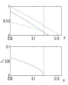
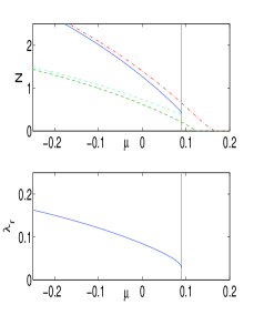
Figure 1: (Color online) The top panels show the norm of the solutions of Eq.(1) for attractive nonlinearity ($s=-1$) as a function of $\mu$ for symmetric (left panel, $x_{0}=0$) and asymmetric double well (right panel, $x_{0}=0.5$). The potential parameters are $\Omega=0.1$, $V_{0}=1$ and $w=0.5$. The solid lines denote the symmetric solution, the dashed-dotted lines denote the antisymmetric one, while the dashed lines denote the asymmetric solutions that are generated from the bifurcation at $\mu_{c}\approx 0.122$ (pitchfork) and $\mu_{c}\approx 0.009$ (saddle-node) respectively. The bottom panels show the maximal real eigenvalue associated with the linear stability of the symmetric branches.

Next, in the same case ($s=-1$), we consider a double well potenial with a weak asymmetry ($x_{0}=0.5$). In this case, the constants involved in Eqs. (6)-(8) are found to be $A_{0}=0.14903$, $A_{1}=0.15618$, $B=0.02958$, $\omega_{0}=0.1249$ and $\omega_{1}=0.16535$, while $\Gamma_{0}=0.0407$ and $\Gamma_{1}=-0.04077$. Note that even such a weakly asymmetric case, renders the right well “shallower”, in the following sense: the density, or power $N$ (regarding the ground state of the linear problem), in the right well is smaller than the one in the left well. Thus, in the nonlinear problem, the respective branches that bear the larger part of the density in the right or in the left well (i.e., the ones having, roughly speaking, the shape of a single pulse in each of the wells) are no longer equivalent. This results in a significant difference between the asymmetric and the symmetric case discussed above, namely there is no longer a pitchfork bifurcation, but instead, there is a saddle-node bifurcation. This result is shown in the top right panel of Fig. 1, where $N$ is shown as a function of $\mu$. It is readily observed that, due to the nature of the saddle-node bifurcation, two branches (one of which is stable and the other one is unstable) “collide” at some critical value of $\mu=\mu_{c}$ (see below) and disappear. These branches are the more “symmetric” one, that has support in both wells (see solid line in top left panel of Fig. 2), and the one pertaining to the state having the form of a single pulse in the shallower well (see dashed line in the rightmost top panel of Fig. 2). The instability of the former branch is depicted in the bottom right panel of Fig. 1, where the maximal real eigenvalue is shown as a function of $\mu$. On the other hand, there exists also another single-pulse branch supported over the deeper well (see top third panel of Fig. 2), which persists all the way to the linear limit. Furthermore, the dash-dotted anti-symmetric branch of the top right of Fig. 1 is shown in the second top panel of Fig. 2.

The novel feature described above, namely the asymmetric breakdown of the pitchfork bifurcation into a saddle-node one, is a particular feature of asymmetric double well potentials that, to the best of our knowledge, has not been previously appreciated. Notice that Eq. (8) predicts that the saddle-node bifurcation occurs at $\mu_{c}=0.08748$, while the numerical result is $\mu_{c}=0.09\pm 0.001$; apparently the two results are again in excellent agreement.

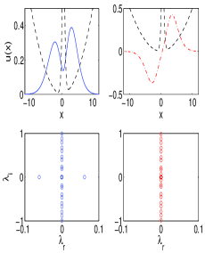
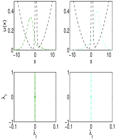
Figure 2: (Color online) The steady state solutions of Eq.(1), (see also Fig. 1) for the focusing, asymmetric case (top panels) and their linear stability (bottom panels) for $\mu=0.05$. The black-dashed line shows the double well potential.

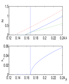
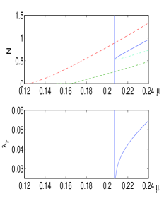
Figure 3: (Color online) Same as in Fig.1 but for the repulsive nonlinearity ($s=+1$). The dashed-dotted lines denote the symmetric solution, the solid the antisymmetric, while the dashed lines denote the asymmetric solutions generated from the bifurcation at $\mu_{c}\approx 0.168$ (pitchfork) and $\mu_{c}\approx 0.207$ (saddle-node) respectively. Contrary to the case $s=-1$, the bifurcations originate from the anti-symmetric branch.

Let us now consider the repulsive nonlinearity ($s=+1$). In this case, for the symmetric potential ($x_{0}=0$), the pitchfork bifurcation still occurs; however, now it does not originate from the symmetric branch, but rather from the anti-symmetric one with $(\rho_{0},\rho_{1})=(0,\sqrt{N})$, giving again rise to symmetry breaking. Analyzing Eq. (8), we find that this occurs when

$$N>N_{c}\geq\frac{\Delta\omega}{3B-A_{1}},$$ (10)

and for $\mu=\omega_{0}+3BN=0.16822$, once again in excellent agreement with the numerical result $\mu_{c}=0.168(\pm 0.001)$.

On the other hand, in the same case ($s=+1$) but for an asymmetric ($x_{0}=0.5$) double well, the bifurcation still originates from anti-phase (between the wells) solutions, but again (as in the asymmetric case with $s=-1$), the bifurcation is of the saddle-node type. This is theoretically predicted to occur at $\mu_{c}=0.21342$, once again in very close agreement to the numerical result $\mu_{c}=0.207\pm 0.001$. The details of the bifurcation diagrams, are illustrated in Fig. 3 (analogously to Fig. 1), while the steady state solutions and their linear stability are shown in Fig. 4 (analogously to Fig. 2).

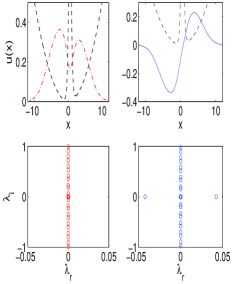
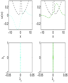
Figure 4: (Color online) The steady state solutions of Eq.(1), (see also Fig. 3) for $s=+1$ in the asymmetric case (top panels) and their linear stability (bottom panels) for $\mu=0.22$. The black-dashed line shows the double well potential.

Conclusions. In conclusion, we have presented a systematic analysis based on a Galerkin, two-mode truncation of the stationary states of symmetric and asymmetric double well potentials. The analysis has been carried out both for repulsive and attractive nonlinearities and, as such, can be relevant to a variety of physical contexts; these include matter-wave physics (most directly), nonlinear optics, as well as other contexts where it is relevant to consider double well potentials in the NLS model proper. We have demonstrated that our analytical approach describes quite accurately, both qualitatively and quantitatively the features of the nonlinear solutions; numerical results were shown to be in excellent agreement with the analytical predictions.

In the case of a symmetric double well potential, it has been shown that a symmetry-breaking (pitchfork) bifurcation of the ground state occurs for attractive nonlinearities, while it is absent for repulsive nonlinearities. It has also been found that a similar bifurcation of the first excited state occurs in the relevant branches for repulsive nonlinearities, oppositely to the case of attractive ones, where such bifurcation does not happen. Additionally, regarding the above feature, we have illustrated that symmetric potentials are very particular (degenerate) due to their special characteristic of mirror-equivalence of the emerging symmetry-breaking states. We have shown that even weak asymmetries lift this degeneracy and lead to saddle-node bifurcations instead of pitchfork ones that were similarly quantified in both attractive and repulsive nonlinearity contexts.

These results underscore the relevance of analyzing steady state features of nonlinear models (in the presence of external potentials) based on the states of the underlying linear equations. It would be particularly interesting to examine the extent to which dynamical features of such models can be captured by similar truncations. Such studies are currently in progress.

Acknowledgements. Constructive discussions with M.K. Oberthaler are kindly acknowledged. This work has been partially supported from “A.S. Onasis” Public Benefit Foundation (G.T.) and NSF (P.G.K.).

References

- (1) C. Sulem and P.L. Sulem, The Nonlinear Schrödinger Equation, (Springer-Verlag, New York, 1999).
- (2) M.J. Ablowitz, B. Prinari and A.D. Trubatch, Discrete and Continuous Nonlinear Schrödinger systems (Cambridge University Press, Cambridge, 2003).
- (3) F. Dalfovo, S. Giorgini, L.P. Pitaevskii, and S. Stringari, Rev. Mod. Phys. 71, 463 (1999).
- (4) P.G. Kevrekidis and D.J. Frantzeskakis, Mod. Phys. Lett. B 18, 173 (2004); V.V. Konotop and V.A. Brazhnyi, Mod. Phys. Lett. B 18 627, (2004).
- (5) Yu.S. Kivshar and G.P. Agrawal, Optical Solitons: From Fibers to Photonic Crystals, Academic Press (San Diego, 2003).
- (6) D. N. Christodoulides, F. Lederer and Y. Silberberg, Nature 424, 817 (2003); J.W. Fleischer et al., Opt. Expr. 13, 1780 (2005).
- (7) S. Raghavan et al., Phys. Rev. A 59, 620 (1999); S. Raghavan et al., Phys. Rev. A 60, R1787 (1999); A. Smerzi and S. Raghavan, Phys. Rev. A 61, 063601 (2000).
- (8) E.A. Ostrovskaya et al., Phys. Rev. A 61, 031601 (R) (2000).
- (9) K.W. Mahmud, J. N. Kutz and W. P. Reinhardt, Phys. Rev. A 66, 063607 (2002).
- (10) V.S. Shchesnovich, B.A. Malomed, and R.A. Kraenkel, Physica D 188, 213 (2004).
- (11) D. Ananikian and T. Bergeman, Phys. Rev. A 73, 013604 (2006).
- (12) P. Ziń et al., Phys. Rev. A 73, 022105 (2006).
- (13) M. Albiez et al., Phys. Rev. Lett. 95, 010402 (2005).
- (14) C. Cambournac et al., Phys. Rev. Lett. 89, 083901 (2002).
- (15) P.G. Kevrekidis et al., Phys. Lett. A 340, 275 (2005).
- (16) E.B. Davies, Commun. Math Phys. 64, 191 (1979)
- (17) R. K. Jackson and M. I. Weinstein, J. Stat. Phys. 116, 881 (2004).
- (18) W. H. Aschenbacher et al., J. Math. Phys. 43, 3879 (2002).
- (19) T. Kapitula and P.G. Kevrekidis, Nonlinearity 18, 2491 (2005).
- (20) C. Raman et al., Phys. Rev. Lett. 83, 2502 (1999); R. Onofrio et al., Phys. Rev. Lett. 85, 2228 (2000).