Nonlinear surface impurity in a semi-infinite 2D square lattice

Abstract

We examine the formation of localized states on a generalized nonlinear impurity located at, or near the surface of a semi-infinite 2D square lattice. Using the formalism of lattice Green functions, we obtain in closed form the number of bound states as well as their energies and probability profiles, for different nonlinearity parameter values and nonlinearity exponents, at different distances from the surface. We specialize to two cases: impurity close to an “edge” and impurity close to a “corner”. We find that, unlike the case of a 1D semi-infinite lattice, in 2D, the presence of the surface helps the formation of a localized state.

An interesting recent development for extended, nonlinear systems with discrete translational invariance is the the concept of “breather” or “intrinsic localized mode”, whose existence is the result of a careful balance between nonlinearity and discretenesskv_pt . These excitations are thought of as generic to a wide range of different physical systems, including Josephson junctionsjunction , biopolymersbio , Bose-Einstein condensates in a magneto-optical trapBE and arrays of nonlinear optical waveguidesDS , among others. In nonlinear optics, these excitations are known as “discrete solitons”(DS) due to their ability to move in a more or less robust manner, when endowed with momentum (beam angle). In fact, many theoretical predictions made for DS have now been experimentally verified in optics, causing a surge of activity in this field. It is believed that an understanding on the creation and propagation of DS under different conditions, might have a substantial impact on future telecomunication/computing systems.

When looking for discrete solitons, one notes that in the limit of high nonlinearity or high power, the effective nonlinearity is concentrated in a few “sites” only and, therefore, it makes sense to make the approximation of replacing the whole nonlinear system for a simpler one, consisting of a discrete linear lattice with a a small nonlinear cluster, or even a single site embedded in it. The simplified system is oftentimes amenable to exact mathematical treatment, leading to closed-form expressions for the relevant energies and nonlinearity parameters, as well as providing a bound state spatial profile for the relevant amplitudes, be these electronic or optical. This high-nonlinearity localized state provides a very good starting point when looking for discrete solitons in a more general, less restrictive context.prb1 ; prb2 .

On the other hand, given the practical need to scale down the components of any all-optical system, such as waveguide arrays, it becomes important to understand how the presence of some realistic effects such as boundaries or surfaces affect the creation and propagation characteristics of these DS. Discrete surface solitons at the edge of a one-dimensional (1D) waveguide array has been predictedmakris and experimentally observedsuntsov . It has been shown that the presence of nonlinearity can stabilize the surface modes in discrete systems, and give rise to different types of states localized at or near a 1D surface, in a vibrationaltakeno or optical contextmvk_OL .

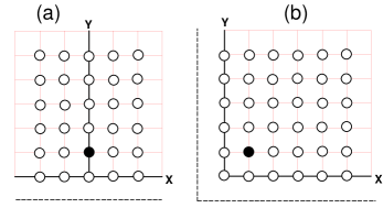
Figure 1: (color online) Nonlinear impurity placed near the “side” (a) and near the “corner” (b) of a semi-infinite square lattice. Along the dashed lines the amplitude is strictly zero.

In this work, we consider surface effects for a simple two-dimensional (2D) system consisting of a nonlinear impurity placed near the boundary of a semi-infinite square lattice(Fig.1), and examine the conditions for the existence of bound state(s), and compare them to the results obtained for 1D case.

The stationary modes of a $D$-dimensional discrete lattice in the presence of a single nonlinear impurity located at ${\bf d}$ are obtained from the stationary-state discrete nonlinear Schrödinger (DNLS) equation

$$-i\beta C_{\bf n}+V\;\sum_{n.n}\;C_{\bf m}+\delta_{{\bf nd}}\chi\;|C_{\bf n}|^{\alpha}\;C_{\bf n}=0$$ (1)

where ${\bf n}$ is a site of a $D$-dimensional lattice, $V$ is the transfer matrix element, $\chi$ is the nonlinearity parameter and $\alpha$ is the nonlinearity exponent. The sum in (1) is usually restricted to nearest-neighbors, but other cases have also been consideredprb_dispersion . In the conventional DNLS case, $\alpha=2$ and $\chi$ is proportional to the square of the electron-phonon coupling at site ${\bf n}$, while $\beta$ is the eigenenergy. In nonlinear optics Eq.(1) describes the transversal dynamics of an optical field in an array of weakly coupled linear waveguides, in the presence of a single, nonlinear (Kerr) waveguide. There, $\alpha=2$, $C_{n}$ is the normalized amplitude of the field in the nth waveguide, while V is the coupling among waveguides and $\chi$ is the effective nonlinearity of the “impurity” waveguide proportional to the nonlinear Kerr coefficient. Also in this case, $\beta$ in Eq.(1) must be understood as the propagation constant for the allowed optical modes along the longitudinal coordinate of the array. Hereafter, for the sake of definiteness, we will work in a condensed matter context, but the results obtained can be applied to nonlinear optics, where appropriate.

I Localized states near the surface of a 2D square lattice

Let us examine the existence of bound states around a single generalized nonlinear impurity located near the surface of a semi-infinite square lattice (Fig.1(a), (b)). We follow in this section the Green function procedure already described in previous worksprb1 ; prb2 , so that the reader already familiar with this formalism can skip this section and proceed directly to the next one. We denote by ${\bf d}=(d_{x},d_{y})$ the position of the impurity. By normalizing all energies to the half bandwidth of the infinite chain case ($4V$), the dimensionless Green function $G=1/(z-H)$ can be formally expanded aseconomou

$$G=G^{(0)}+G^{(0)}H_{1}G^{(0)}+G^{(0)}H_{1}G^{(0)}H_{1}G^{(0)}+\cdots$$ (2)

where $G^{(0)}$ is the unperturbed ($\chi=0$) Green function of the semi-infinite lattice and $H_{1}=\gamma|C_{\bf d}|^{\alpha}|{\bf d}\rangle\langle{\bf d}|$, with $\gamma\equiv\chi/4V$. Series (2) can be resumed to all orders to yield

$$G_{{\bf m}{\bf n}}=G_{{\bf m}{\bf n}}^{(0)}+{\gamma|C_{{\bf d}}|^{\alpha}G_{{\bf m}{\bf d}}^{(0)}G_{{\bf d}{\bf n}}^{(0)}\over{1-\gamma|C_{{\bf d}}|^{\alpha}G_{{\bf d}{\bf d}}^{(0)}}},$$ (3)

where $H_{{\bf m}{\bf n}}\equiv\langle{\bf m}|G|{\bf n}\rangle$. The energy of the bound state(s) is obtained form the poles of $G_{{\bf m}{\bf n}}$, i.e., by solving

$$1=\gamma|C_{{\bf d}}|^{\alpha}G_{{\bf d}{\bf d}}^{(0)}(z_{b}),$$ (4)

while the bound state amplitudes $C_{{\bf n}}$ are obtained form the residues of $G_{{\bf m}{\bf n}}$ at $z=z_{b}$:

$$|C_{{\bf d}}|^{2}=-{G_{{\bf n}{\bf d}}^{(0)}(z_{b})G_{{\bf d}{\bf n}}^{(0)}(z_{b})\over{{G^{\prime}}_{{\bf d}{\bf d}}^{(0)}(z_{b})}}$$ (5)

Inserting this back into the bound state energy equation leads to a nonlinear equation for the eigenenergies:

$${1\over{\gamma}}={{G_{{\bf d}{\bf d}}^{(0)}}^{\alpha+1}(z_{b})\over{[-G_{{\bf d}{\bf d}}^{{}^{\prime}(0)}(z_{b})]^{\alpha/2}}}.$$ (6)

The unperturbed Green function $G_{{\bf m}{\bf n}}^{(0)}$ for the semi-infinite lattice, can be calculated by a judicious application of the method of mirror images, as we will show in the next two sections.

II Impurity close to an “edge”

We start by placing the impurity near the edge of the lattice as depicted on Fig.1(a). In order to simplify matters, we take ${\bf d}=(0,d)$. Since there is no lattice below $(0,0)$, $G_{{\bf m}{\bf n}}^{(0)}$ should vanish identically along the sites lying on the dashed line in Fig.1(b). This implies,

$$G_{{\bf d}{\bf d}}^{(0)}=G_{{\bf d}{\bf d}}^{\infty}-G_{{\bf d},{-{\bf d}-2{\bf j}}}^{\infty}.$$ (7)

where ${\bf j}$ is a unit vector in the $y$-direction and where $G_{{\bf m}{\bf n}}^{\infty}$ refers to the Green function of the infinite 2D square lattice. Now, using the translation invariance property $G_{{\bf m}{\bf n}}^{\infty}=G_{{\bf m}-{\bf n}}^{\infty}$, and the symmetry $G_{{\bf m}{\bf n}}^{\infty}=G_{{\bf n}{\bf m}}^{\infty}$, we have $G_{{\bf d}{\bf d}}^{\infty}=G_{{\bf 0}{\bf 0}}^{\infty}$ and $G_{{\bf d},{-{\bf d}-2{\bf j}}}^{\infty}=G_{{\bf 0},{2{\bf d}+2{\bf j}}}^{\infty}$ or, using a simplified notation,

$$G_{{\bf d}{\bf d}}^{(0)}=G(z;0,0)-G(z;0,2d+2)$$ (8)

where $G(z;m,n)$ refers to the Green function for an infinite square lattice

$$G(z;m,n)={1\over{\pi^{2}}}\int_{0}^{\pi}d\phi_{1}\int_{0}^{\pi}d\phi_{2}{\cos(m\phi_{1})\cos(n\phi_{2})\over{z-(1/2)(\cos(\phi_{1})+\cos(\phi_{2}))}}$$ (9)

(see, for instance, ref.morita ). We note that (8) is identically zero at $d=-1$. The computation of $G(z;0,d)$ and $G(z;0,2d+2)$ can be achieved by using some recurrence relationsmorita by means of which, an arbitrary Green function $G(z;m,n)$ can be expressed in terms of two Green functions only: $G(z;0,0)$ and $G(z;1,1)$, where $G(z;0,0)=(2/\pi z)K[1/z^{2}]$ and $G(z;1,1)=(2/\pi z)(\ (2z^{2}-1)K[1/z^{2}]-2z^{2}E[1/z^{2}]\ )$, where $K[x]$ is the complete elliptical integral of the first kind: $K[x]=\int_{0}^{\pi/2}[1-x\sin(\phi)^{2}]^{-1/2}d\phi$, and $E[x]$ is the complete elliptical integral of the second kind: $E[x]=\int_{0}^{\pi/2}[1-x\sin(\phi)^{2}]^{1/2}d\phi$. In this way, we have obtained a number of non-diagonal Green functions in explicit form (see Appendix I). In particular, we have obtained $G(z;0,2)$, $G(z;0,4)$ and $G(z;0,6)$ and $G(z;0,6)$ in closed form, needed in Eq.(8). We finally insert (8) into the RHS of the eigenvalue equation, Eq.(6), and solve for $z_{b}$ numerically. However, the most important features can be already deduced from the structure of Eq.(6): In Fig.2 we show

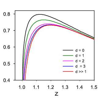
Figure 2: (color online) Impurity close to edge: Right-hand side of Eq.(6) versus $z$, for $\alpha=2$ and for different distances from the “edge”.

the right-hand side of Eq.(6), for the important case $\alpha=2$ (standard DNLS) and for different $d$ values. For comparison, the case $d\rightarrow\infty$ has also been included. Since it is the intersection of these curves with the horizontal line $1/\gamma$ what determines the existence of bound states, we see that in general, for finite $d$ a minimum value of nonlinearity $\gamma$ is needed to create a bound state. An increase past the threshold value creates two bound states. One of these tends to approach the band while the other departs from the band as $\gamma$ is increased. As argued before in previous worksprb1 ; prb2 , the former should correspond to an unstable localized state, while the latter denotes a stable bound state.

In Fig. 3 we show a bound state phase diagram in nonlinearity strength-nonlinearity exponent space, showing the number of bound states, for different positions of the impurity. As the impurity is brought more and more inside the lattice, the region in parameter space where two bound states are possible increases. In the limit $d\rightarrow\infty$, the curve where a single bound state is found, touches the origin, and coincides with the curve for an infinite square lattice computed in a previous workmm_prb_square , as expected.

An interesting question now is, how does the critical nonlinearity to form a localized state $\gamma_{c}$ depend on $d$? Such critical nonlinearity value is formally given by the inverse of the RHS of Eq.(6), evaluated at precisely the value of $z$ where the RHS of Eq.(6) possesses a maximum. In Fig. 4 we show $\gamma_{c}$ versus $d$, for a variety of nonlinearity exponents. As $d$ is increased past $3$, all curves seem to converge pretty quickly to their asymptotic values.

The situation depicted in Figs.3 and 4 is qualitatively similar to what one encounters when placing a nonlinear impurity near the edge of a semi-infinite 1D latticeprb1 , with a difference, though: In the 1D case, for $\alpha=2$ the presence of the surface tended to increase $\gamma_{c}$, while in our case, the proximity of the “edge” tends to decrease $\gamma_{c}$: its presence helps localization of the excitation. We also observe that, for a given impurity position $d$, the nonlinearity needed to create a bound state increases with $\alpha$. This was also observed in 1D and the explanation is quite general, independent of dimensionality: From Eq.(1) we see that, since $|C_{n}|<1$, as $\alpha$ is increased,$|C_{n}|^{\alpha}$ will necessarily decrease, meaning that a larger value of $\gamma$ will be needed to keep the value of the effective impurity strength, $\gamma|C_{\bf d}|^{\alpha}$.

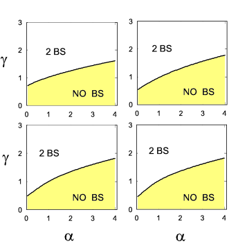
Figure 3: (color online) Bound state phase diagrams in nonlinearity parameter-nonlinearity exponent, for impurity placed at different distances from the “edge”: $d=0$(top left), $d=1$ (top right), $d=2$ (bottom left) and $d=3$ (bottom right). On the solid curve, there is precisely one bound state.

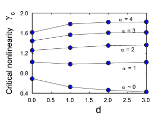
Figure 4: (color online) Scaled critical nonlinearity for onset of bound state as a function of the distance from the nonlinear impurity to the “edge” of the lattice, for several nonlinearity exponents, ranging from $\alpha\approx 0$ up to $\alpha=4$.

III Impurity close to a “corner”

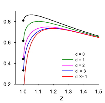
Figure 5: (color online) Impurity close to corner: Right-hand side of Eq.(6) versus $z$, for $\alpha=2$ and for different distances along the diagonal.

In this case, the impurity is located near the corner of the lattice as depicted on Fig.1(b). In order to simplify matters, we take ${\bf d}=(d,d)$; i.e., we place the impurity along the “diagonal” sites. In this case because the impurity is surrounded by “more surface” than in the previous case, one would expect even stronger departures from the 1D results already explored in refs.prb1 ; prb2 . Since there is no lattice to the left or below $(0,0)$, $G_{{\bf m}{\bf n}}^{(0)}$ should vanish identically along the sites lying on the dashed line in Fig.1(a). Thus,

$$G_{{\bf d},{\bf d}}^{(0)} = G_{{\bf d},{\bf d}}^{\infty}-G_{{\bf d},(d_{x},-d_{y}-2)}^{\infty}$$ (10)

$$-G_{{\bf d},(-d_{x}-2,d_{y})}^{\infty}+G_{{\bf d},(-d_{x}-2,-d_{y}-2)}^{\infty}$$

We can recast Eq.(10) as

$$G_{{\bf d}{\bf d}}^{(0)}(z)=G(z;0,0)-2G(z;0,2d+2)-G(z;2d+2,2d+2)$$ (11)

where $G(z;m,n)$ is given by Eq.(9). On Fig.5 we show the right-hand side of Eq.(6), for the important case $\alpha=2$ (standard DNLS) and for different $d$ values. For comparison, the case $d\rightarrow\infty$ has also been included. We note an important difference with the case of the previous section: As $z\rightarrow 1^{+}$, the RHS of Eq.(6) approaches a finite, non-zero value. This implies the following: An increase past a minimum value of nonlinearity $\gamma_{c}^{(1)}$ creates two bound states. One of these tend to depart from the band while the other approaches the band as $\gamma$ is increased. The former state is stable while the latter is unstable and, in fact ceases to exist altogether when $\gamma$ reaches a second critical value $\gamma_{c}^{(2)}$, marked with a dot on Fig.5. Afterwards, there is only a single bound state. The value of this second critical nonlinearity can be obtained in closed form by taking the limit $z\rightarrow 1^{+}$ in Eq.(6)(see Appendix II). In this way,we have obtained:

$$\gamma_{c}^{(2)}(d=0) = 1.236,\hskip 14.22636pt\gamma_{c}^{(2)}(d=1)=1.626$$

$$\gamma_{c}^{(2)}(d=2) = 2.267,\hskip 14.22636pt\gamma_{c}^{(2)}(d=3)=3.01$$ (12)

As $d$ increases, this critical nonlinearity parameter increases rapidly, and tends to diverge for $d\rightarrow\infty$, that is, for an infinite square lattice, the unstable bound state will still be present at arbitrarily large nonlinearity parameter values, a well-known factmm_prb_square .

In Fig. 6 we show bound state phase diagrams in nonlinearity strength-nonlinearity exponent space, showing the number of bound states, for different positions of the impurity. As the impurity is brought more and more inside the lattice, the region in parameter space where two bound states are possible increases. In the limit $d\rightarrow\infty$, the region comprising one bound state will get more and more “squeezed” into the $\gamma$ axis and will formally disappear for a truly infinite square latticemm_prb_square .

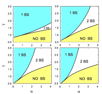
Figure 6: (color online) Bound state phase diagrams in nonlinearity parameter-nonlinearity exponent, for impurity placed at different (diagonal) distances from the “corner”: $d=0$(top left), $d=1$ (top right), $d=2$ (bottom left) and $d=3$ (bottom right).

In Fig.7 we show $\gamma_{c}^{(1)}$ versus $d$, for a variety of nonlinearity exponents. We note that, as the impurity is brought closer and closer to the “corner”, $\gamma_{c}^{(1)}$ increases or decreases, depending on whether $\alpha$ is above or below, approximately, two. This feature was also present in the previous case (see Fig.4). However, in this case, the proximity effect of the corner is much more pronounced. In particular, as the impurity is brought closer to the corner, the nonlinearity needed to create a bound state decreases even more than when the impurity is brought closer to the edge. This implies an even greater departure from the 1D results. As $d$ is increased past $3$, all curves seem to start converging towards their asymptotic values.

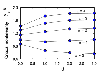
Figure 7: (color online) Scaled critical nonlinearity for onset of bound state as a function of the distance from the nonlinear impurity to “corner” of the lattice, for several nonlinearity exponents, ranging from $\alpha\approx 0$ up to $\alpha=4$.

IV Conclusion

We have examined the formation of bound states around a general nonlinear impurity located at, or near the “edge” or the “corner” of a semi-infinite 2D square lattice. By means of the lattice Green functions formalism, we have obtained in closed form the nonlinear equation for the bound state energies, from which we have obtained bound state phase diagrams in nonlinearity strength-nonlinearity parameter, for different impurity positions with respect to the surface. In general, one finds that, a minimum value of nonlinearity is needed to create a bound state. Up to two bound states are possible, although only one of them is always unstable. These features have been observed previously for the 1D semi-infinite system. However, for the standard DNLS case ($\alpha=2$), some interesting departures from the 1D case were also found: (i) The increased number of surface sites surrounding the impurity when it is close to the “corner” seem to obliterate completely the unstable bound state, for relatively high nonlinearity values. (ii) As the impurity is brought closer to the surface, the nonlinearity needed to create a localized state decreases, specially in the case when the impurity is near a “corner”. This suggests that, in a more general context, when considering the creation of discrete solitons near the surface of a completely nonlinear (Kerr) 2D square lattice, the surface (edge, corner) of the square lattice would exert an attractive potential, instead of the repulsive one observed in semi-infinite 1D systemsmvk_OL . This would make the creation of discrete solitons easier to accomplish and observe near the boundaries of 2D discrete periodic systems.

V Acknowledgments

This work was partially supported by Fondecyt grants 1050193 and 7050173. The author is grateful to Y. S. Kivshar for useful discussions.

VI APPENDIX I

For an infinite square lattice there are a number of recursion relations that allow one to express any desired Green function, in terms of , ultimately two basic ones. We state some recursion relations (see for instance, Moritamorita ). For the sake of space, we drop mention of the re-scaled frequency $z$ inside the argument of the Green functions and define:

$$A\equiv G(0,0)={2\over{\pi z}}K[1/z^{2}]$$ (13)

$$B=G(1,1)={2\over{\pi z}}[\ (2z^{2}-1)K[1/z^{2}]-2z^{2}E[1/z^{2}]\ ]$$ (14)

and use the relations:

$$G(1,0) = zG(0,0)-1$$ (15)

$$G(m+1,m+1) = {4m\over{2m+1}}(2z^{2}-1)G(m,m)$$ (16)

$$-{2m-1\over{2m+1}}G(m-1,m-1)$$

$$G(m+1,m) = 2zG(m,m)-G(m,m-1)\ \ \ \$$ (17)

$$G(m+1,n) = 4zG(m,n)-G(m-1,n)$$ (18)

$$-G(m,n+1)-G(m,n-1)$$

$$G(m+1,0) = 4zG(m,0)-G(m-1,0)$$ (19)

$$-2G(m,1)$$

Using these relations, one obtains:

$$G(0,1)=Az-1$$ (20)

$$G(0,2)=-2\,B-4\,z+A\,\left(-1+4\,z^{2}\right)$$ (21)

$$G(1,2)=1-A\,z+2\,B\,z$$ (22)

$$G(0,3)=-1-12\,B\,z-16\,z^{2}+A\,z\,\left(-3+16\,z^{2}\right)$$ (23)

$$G(2,2)=(1/3)(-A-4\,B+8\,B\,z^{2})$$ (24)

$$G(0,4)=$$ (26)

$$(1/3)A(-5+192\,z^{4})$$

$$-(8/3)(B+22\,B\,z^{2}+6\,(z+4\,z^{3}))$$

$$G(1,3)=(4/3)(A+6\,z-6\,A\,z^{2}+B((7/4)+4\,z^{2}))$$ (27)

$$G(2,3)=(1/3)(-3+A\,z+2\,B\,z\,(-7+8\,z^{2}))$$ (28)

$$G(3,3)=\frac{-3\,B}{5}+\frac{8\,\left(-1+2\,z^{2}\right)\,\left(-A-4\,B+8\,B\,z^{2}\right)}{15}$$ (29)

$$G(1,4) = 1+48\,z^{2}+8\,B\,z\,(3+2\,z^{2})$$ (30)

$$+A(9\,z-48\,z^{3})$$

$$G(3,4) = 1+(1/15)A(11\,z-32\,z^{3})$$ (31)

$$+(4/15)B\,z\,(29-84\,z^{2}+64\,z^{4})$$

$$G(4,4) = (64/105)A(-(71/64)+6\,z^{2}-6\,z^{4})$$ (32)

$$+(8/105)B(-(11/32)+(59/16)\,z^{2}$$

$$-9\,z^{4}+6\,z^{6})$$

$$G(0,5) = (16/3)48\,z^{4}\,(-1+A\,z)$$ (33)

$$+(1/48)(-3-65\,A\,z-140\,B\,z)$$

$$+(1/3)z^{2}\,(-27+15\,A\,z-50\,B\,z)$$

$$G(2,4) = (1/15)A\,(-23+156\,z^{2})-(180/15)z$$ (34)

$$+(B/15)(-19-136\,z^{2}+96\,z^{4})$$

$$G(1,5) = 8z(3+32\,z^{2})+(1/15)A(28+504\,z^{2}-3840\,z^{4})$$ (35)

$$+(1/15)B(43+2512\,z^{2}+768\,z^{4})$$

$$G(0,6) = (1/15)A(-31-2308\,z^{2}+11520\,z^{4}+15360\,z^{6})$$ (36)

$$-(2/15)(30\,z\,(9+256\,z^{2}+256\,z^{4})$$

$$+(1/15)B(23+3472\,z^{2}+8768\,z^{4})$$

VII APPENDIX II

For an impurity close to a “corner”, there is a critical nonlinearity value $\gamma_{c}^{(2)}$, beyond which, the unstable bound state ceases to exist. It can be computed by taking the limit $z_{b}\rightarrow 1^{+}$ in Eq.(6), with the Green functions obtained in section II. In this way, we have obtained:

$$\gamma_{c}^{(2)}(d=0) = {27\over{64}}\pi^{2}{(4-\pi)\over{(3\pi-8)^{3}}}=1.236$$

$$\gamma_{c}^{(2)}(d=1) = {8575\pi^{2}(65\pi-208)\over{1024(544-175\pi)^{3}}}=1.626$$

$$\gamma_{c}^{(2)}(d=2) = {132068475\pi^{2}(647955\pi-2037676)\over{64(5668760-1805265\pi)^{3}}}=2.267$$

$$\gamma_{c}^{(2)}(d=3) = {6087156075\pi^{2}(74669595\pi-234592192)\over{16384(132029312-42026985\pi)^{3}}}$$

$$=3.01$$

References

- (1) David K. Cambpell, Sergei Flach, and Yuri S. Kivshar, Physics Today 57, 43 (2004).
- (2) L. M. Floria , J. L. Marin , P. J. Martinez , F. Falo and S. Aubry, Europhys. Lett. 36, 539 (1996); E. Trias, J. J. Mazo and T. P. Orlando, Phys. Rev. Lett. 84, 741 (2000); P. Binder, D. Abraimov, A. V. Ustinov, S. Flach and Y. Zolotaryuk, Phys. Rev. Lett. 84, 745 (2000); A. Ustinov, Chaos 13, 716 (2003).
- (3) A. Xie, Lex van der Meer, Wouter Hoff and Robert H. Austin, Phys. Rev. Lett. 84, 5435 (2000); T. Dauxois, M. Peyrard, in Nonlinear Excitations in Biomolecules, M. Peyrard, ed., Springer, New York (1995), p. 127; J. C. Eilbeck, P. S. Lomdahl and A. C. Scott, Physica D 16,318 (1985); A.C. Scott, Phys. Rep. 217, 1 (1992); A. Scott, Nonlinear Science: Emergence and Dynamics of Coherent Structures, 2nd ed., Oxford U. Press, New York (2003); G. P. Tsironis, M. Ibanes and J. M. Sancho, Europhys. Lett. 57, 697(2002); S. F. Mingaleev, Y. B. Gaididei, P. L. Christiansen and Y. S. Kivshar, Europhys. Lett. 59, 403 (2002).
- (4) A. Trombettoni and A. Smerzi, Phys. Rev. Lett. 86, 2353 (2001); J. Phys. B 34, 4711 (2001); A. Smerzi, A. Trombettoni, P.G. Kevrekidis, and A.R. Bishop, Phys. Rev. Lett. 89, 170402 (2002).
- (5) D. N. Christodoulides, R. I. Joseph, Opt. Lett. 13, 794 (1988); Y. S. Kivshar, Opt. Lett. 18, 1147 (1993); H. S. Eisenberg, Y. Silberberg, R. Morandotti, A. R. Boyd, and J. S. Aitchison, Phys. Rev. Lett. 81, 3383 (1998); R. Morandotti, U. Peschel, J. S. Aitchison, H. S. Eisenberg and Y. Silberberg Phys. Rev. Lett. 83, 2726 (1999) and 83, 4756 (1999).
- (6) K. G. Makris, S. Suntsov, D. N. Christodoulides, G. I. Stegeman and A. Hache, Opt. Lett. 30, 2466 (2005).
- (7) S. Suntsov, K. G. Makris, D. N. Christodoulides, G. I. Stegeman, A. Hache, H. Yang, G. Salamo and M. Sorel, Phys. Rev. Lett. 96, 063901 (2006).
- (8) Yu. S. Kivshar, F. Zhang, and S. Takeno, Physica D 119, 125 (1998).
- (9) M. Molina, R. Vicencio, and Yu. S. Kivshar, Opt. Lett. 31 (2006), in press.
- (10) M. I. Molina, Phys. Rev. B 71, 035404 (2005).
- (11) M. I. Molina, Phys. Rev. B 73, 014204 (2006).
- (12) M. I. Molina, Phys. Rev. B 67, 054202 (2003).
- (13) E. N. Economou, Green s Functions in Quantum Physics, Springer Series in Solid State Physics (Springer-Verlag, Berlin, 1979), Vol. 7.
- (14) T. Morita, J. Math. Phys. 12, 1744 (1971).
- (15) M.I. Molina, Phys. Rev. B 60, 2276, (1999).