Bubble break-off in Hele-Shaw flows
Singularities and integrable structures

Abstract

Bubbles of inviscid fluid surrounded by a viscous fluid in a Hele-Shaw cell can merge and break-off. During the process of break-off, a thinning neck pinches off to a universal self-similar singularity. We describe this process and reveal its integrable structure: it is a solution of the dispersionless limit of the AKNS hierarchy. The singular break-off patterns are universal, not sensitive to details of the process and can be seen experimentally. We briefly discuss the dispersive regularization of the Hele-Shaw problem and the emergence of the Painlevé II equation at the break-off.

I Introduction

A Hele-Shaw cell is a narrow gap filled with an incompressible viscous liquid. When another incompressible fluid with low viscosity is injected into the cell, two immiscible liquids form a sharp interface which can be manipulated by pumping in or out the fluids. The motion of the interface is called Hele-Shaw flow and it belongs to a large class of processes referred to as Laplacian growth (LG) review . The latter describes the evolution of two dimensional domains where the normal velocity of the boundary is proportional to the conformal measure — the gradient of the conformal map of the domain taken at the boundary. The dynamics of the interface is unstable; An originally smooth interface tends to evolve into a complicated and highly curved finger-like shape consisting of a collection of near-singularities Sharon .

Recent progress in the study of Laplacian growth is due to the uncovering the integrable structure of the problem and linking to the universal Whitham hierarchy of soliton theory M-WWZ ; WZ ; KM-WWZ ; Shock ; Teo2 ; TW . The signatures of the integrable structure of the problem had appeared earlier in the seminal works R ; Ri ; BS ; 186:Howison ; Mineev ; Why . The integrable structure brings the Laplacian growth into a wider context of mathematical problems appearing in the theory of nonlinear-waves, and recently in random matrix theory and string theory. The relations between the integrable hierarchy and Hele-Shaw flow are transparent and geometrically illustrative and, therefore, the Hele-Shaw flow may serve as an intuitive geometric interpretation of the formal algebraic objects appearing in the theory of non-linear waves and string theory (for a recent development see Shih ). The relations read: (i) the real section of the spectral curve—the central object in Whitham theory—happens to be the interface in the Hele-Shaw flow, and (ii) the cusp-like singularities of the interface are linked to shock-waves of dispersive non-linear waves.

Soliton theory provides a framework for the study and the classification of singularities emerging in Hele-Shaw flows. A universal properties close to a separated singularity is described by a certain reduction of a more general hierarchy. For instance, some cusp-like singularities were recently identified with the KdV hierarchy Teo2 ; Shock and modified-KdV hierarchy TW , and have been studied in this framework.

In this paper we study another class of singularities in the Hele-Shaw flow: those arising at the break-offs—the processes where one bubble with low viscosity breaks into two. We describe the break-off and show that it is a solution of dispersionless limit of the AKNS hierarchy (dAKNS). Curiously, the breaking interface has emerged as a target space in the minimal superstring theory Shih2 .

As a natural extension of the result, we discuss the dispersive regularization of the singularities and the emergence of the Painléve II equation. In the next section, we suggest an experimental set-up where the surface tension and other suppressing mechanisms of singularities are negligible, so that the universal singular behavior at the break-off can be achieved experimentally.

II Set-up and results

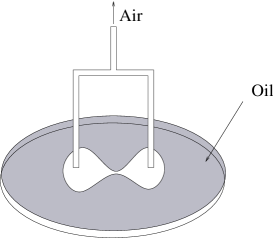
Figure 1: A scheme of an experiment where air is drawn from the air bubble surrounded by oil. A simply connected bubble pinches-off and eventually breaks-off through a singular neck. After the break-off both bubbles are maintained at the same pressure. The singular shape of the neck is universal; It does not depend on the shape of the original bubble.

A Hele-Shaw cell is a narrow gap between two plates filled with incompressible viscous fluid, say oil. Another immiscible and relatively inviscid fluid, say air, occupies part of the cell forming one or several bubbles. Most commonly the flow is produced when air is injected into the cell through a single point in the cell, pushing oil away to the border of the cell. Here we will study a different process: air is extracted from the air bubble—that already exists in the cell—from two fixed points of the cell situating in the bubble as depicted in Fig. 1. As the air is drawn out, a simply-connected air bubble will break into two. The set-up is designed such that the two separate bubbles after the break-off maintain the same pressure. This condition is important.

The Hele-Shaw flow is driven by D’Arcy’s law: velocity in the oil domain is proportional to the gradient of the pressure:

$$\vec{v}=-\frac{b^{2}}{12\mu}\vec{\nabla}P.$$ (1)

The coefficients are the separation of the plates, $b$ and the viscosity of oil, $\mu$. Below we set the pre-factor $\frac{b^{2}}{12\mu}$ to $\frac{1}{2}$, and set the flux-rate such that the area of the air bubble is $\pi t$ where $t$ is the time of the process in the traditional Hele-Shaw flow; $t$ flows backwards in time in our experimental set-up. As the oil is incompressible the pressure is a harmonic function in the oil domain. Inside the air bubble the pressure is a constant (which may be set to zero) in time and space. If the surface tension is negligible then the pressure is continuous across the boundary. These set up a Dirichlet boundary problem:

$$\Delta P=0\;\;\mbox{in oil},\quad P=0\;\;\mbox{on the interface},\quad P\to-\log|z|\;\mbox{ at }z\to\infty,$$ (2)

where we followed the conventional setup of injection. $z=x+iy$ is the complex coordinate.

A comment about surface tension is in order. In the case of an expanding interface, when the air is injected into the cell, almost every initial shape of the interface results in a cusp-like singularity at some finite time, if the surface tension and any other damping mechanism is neglected. After this time the problem defined by Eqs. 1 and 2 is ill-posed. Introduction of a damping mechanism (such as surface tension Tanveer ) usually ruins the analytical and integrable structure of the problem. The only exception, where the singularities are curbed, is the situation proposed in recent papers Teo2 ; Shock .

However, the reverse process, which we consider in this paper, is well defined (section 7 of Shock ). Before the break-off the interface remains smooth regardless of how thin the neck is. Remarkably the problem remains well defined even after the break-off when the tips of the two emergent bubbles are highly curved. This is true when the two bubbles are kept at the same pressure, which motivates the design of the cell as in Fig. 1. In this case, the surface tension can be safely neglected by increasing the extraction rate. This is perhaps the only case that the singularities can be regularized without resorting to a damping mechanism and thus preserving the analytic structure of the zero surface tension problem.

We will show that the singular behavior of the neck at the break-off falls into universal classes characterized by two even integers $(p,q)=(4n,2),\;n=1,2,\cdots$, and only by a finite number ($2n$) of parameters. They are called deformation parameters. While, an infinite number of remaining parameters characterizing the interface become irrelevant in the vicinity of the break-off: the break-off is universal. The deformation parameters are the flows of the integrable hierarchy.

Figure 2: Typical break-off of two droplets at successive time slices.

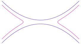
Figure 3: Local curves of (4,2)-break-off just before and after the break-off.

In Cartesian coordinates the shape of the neck reads:

$$y^{q}=x^{p}F_{p,q}\left(\frac{|t|^{\Delta_{pq}}}{x}\right),$$

where we translate the time $t$ such that $t=0$ corresponds to the break-off point. In this paper we consider only $(p,q)=(4n,2)$ with $n$ being a positive integer. We have obtained $\Delta_{4n,2}=\frac{1}{2n}$. The function $F_{4n,2}$, a polynomial of degree $4n$ at most, is characterized by $2n$ parameters. Two of these parameters may be eliminated by re-scaling the coordinates. For example, in the most generic case of $(4,2)$-break-off, shown in Fig. 3, the function reads

$$F_{4,2}(\xi)=\begin{cases}\left(1+\frac{1}{2}\xi^{2}\right)^{2},\quad~{}t>0:\mbox{before break-off}\\ 1-\xi^{2}~{},\quad\quad\quad t<0:\mbox{after break-off}\end{cases}.$$

The same curve will appear as the spectral curve of the AKNS hierarchy.

III Global solutions

Before emphasizing the singular behavior at the break-off, we start by a general description of Hele-Shaw processes from a global standpoint. We start from the case of an arbitrary genus (the genus is the number of bubbles minus one). Then we specify it to the case of two bubbles using elliptic functions. In this section we employ a traditional approach of describing the evolution by a set of moving poles of an analytical function mapping the exterior of the air bubbles to a standard domain. This approach has been developed in R ; Ri ; BS ; Mineev . It does not appeal to the notion of integrablilty.

III.1 The Schwarz function

Let us consider a bounded, multiply connected domain ${\sf D}$ in the complex plane (a Hele-Shaw cell). The domain is occupied by an incompressible fluid with negligible viscosity (air bubbles). Unbounded exterior of the domain, $\mathbb{C}\setminus{\sf D}$, is occupied by an incompressible fluid with high viscosity (oil). Each air bubble contains a source through which air can be drawn out of (supplied into) the bubble such that all bubbles are kept at an equal pressure. Another neutralizing source is placed at infinity.

We will assume that the domain ${\sf D}$ is an algebraic or quadrature domain Quadratures , or, more generally, an Abelian domain Why . These domains are defined by the nature of the Cauchy transform,

$$h(z)=\frac{1}{\pi}\int_{\mathbb{C}\setminus{\sf D}}\frac{d^{2}w}{z-w}=\begin{cases}h^{+}(z)\quad\quad\quad\mbox{at}~{}~{}z\in{\sf D}\\ \overline{z}+h^{-}(z)\quad\mbox{at}~{}~{}z\in\mathbb{C}\setminus{\sf D}\end{cases}.$$ (3)

For quadrature domains the function $h^{+}$ is rational: containing a finite number of poles. For Abelian domains $\partial h^{+}$ is rational and $h^{+}$ may have logarithmic singularities. The use of Abelian domains is not very restrictive; Any domain with a smooth boundary is known to be a limit of Abelian domains Gus —the set of Abelian domain is dense.

The main property of Abelian domains is: the analytical continuations of the function $\bar{z}$ from different connected pieces of the boundary to the exterior $\mathbb{C}\setminus{\sf D}$ give the same result. The function being obtained by this procedure is called a Schwarz function Davis ; Shapiro . In terms of the Cauchy transform (3),

$$S(z)=h^{+}(z)-h^{-}(z).$$

If the boundary is smooth, the Schwarz function can be analytically continued on some strip inside the domain ${\sf D}$.

To fix the notations and emphasize the analytical structure of the Schwarz function in $\mathbb{C}\setminus{\sf D}$ we write

$$S(z)\sim\sum_{k=1}^{K}\frac{\mu_{k}}{(z-q_{k})^{h_{k}}}+\sum_{l=1}^{L}\mu_{K+l}\log(z-q_{K+l})$$ (4)

where $\sim$ stands for an asymptotic equality near each of the singularities $q_{k}\in\mathbb{C}\setminus{\sf D}$ for $k=1,\cdots,K+L$. $h_{k}$’s are positive integers.

The evolution of the domain is determined by the holomorphic function,

$$\phi(z)=\xi(x,y)+ip(x,y),$$

where $\xi$ is stream function and $p$ is the pressure. In terms of $\phi(z)$ and the Schwarz function, D’Arcy’s law reads,

$$\partial_{t}S(z)=i\partial\phi(z).$$ (5)

An immediate consequence is that the Schwarz function behaves at infinity as,

$$\partial_{t}S(z)\sim\overline{q}_{0}+\frac{\overline{\mu}_{0}}{z}\quad\mbox{at}~{}~{}z\rightarrow\infty,\quad q~{}~{}\mbox{is constant and}~{}~{}\partial_{t}\overline{\mu}_{0}=1.$$ (6)

which follows form the boundary condition $\partial\phi(z)\to-i/z$ at infinity. Another consequence is: $h^{+}$ does not depend on time (the proof is in Appendix A):

$$\partial_{t}h^{+}(z)=0.$$

Therefore the parameters in (4) are fixed and can be used as the initial data for the domain.

For a single bubble, these data are sufficient to determine the evolution. For a domain consisting of $g+1$ bubbles, additional $g$ parameters are required KM-WWZ ; they are, for examples, relative areas of the bubbles, pressure differences in the bubbles, or a mixture of the two. Although later we will focus on the equal pressure case, here we do not demand this.

III.2 Dispersionless string equation

D’Arcy’s law written in (5) acquires another important form if the univalent function $\phi$ rather than $z$ is chosen as a coordinate:

$$\frac{\partial S}{\partial\phi}\frac{\partial z}{\partial t}-\frac{\partial S}{\partial t}\frac{\partial z}{\partial\phi}=-i.$$ (7)

Here the derivative in time is taken at fixed $\phi$. This form is known as the dispersionless string equation.

Figure 4: Two distant points $A$ and $B$ along the boundary become close at the break-off. A blow-up of the critical break-off region is plotted. Dotted lines are the interfaces when the bubble breaks up.

A Cartesian form of this equation is convenient to study break-off. Let us choose a coordinate system where the origin is at the pinch-off point and the $x$ axis is tangent to the interface at the pinch-off (the dashed lines in Fig. 4). It is convenient to use the following variables.

$$\tilde{x}(z)\equiv\frac{1}{2}(z+S(z)),\quad\tilde{y}(z)\equiv\frac{1}{2i}(z-S(z)).$$

Note that $\tilde{x}$ and $\tilde{y}$ are not Cartesian coordinates of the physical plane; They are holomorphic functions defined outside the bubble and analytical in some vicinity of the boundary. At the interface, however, $\tilde{x}$ and $\tilde{y}$ are equal to its Cartesian coordinates. Using the new variables (with a rescaling of time), Eq. 7 is written as

$$\{\tilde{y},\tilde{x}\}\equiv\frac{\partial\tilde{y}}{\partial\phi}\frac{\partial\tilde{x}}{\partial t}-\frac{\partial\tilde{y}}{\partial t}\frac{\partial\tilde{x}}{\partial\phi}=1.$$ (8)

And equivalently,

$$\partial_{t}\tilde{y}(\tilde{x})=-\partial_{\tilde{x}}\phi(\tilde{x}).$$ (9)

This form of the evolution equation appeared long ago in Kochina . It was recognized in M-WWZ as the dispersionless string equation known in soliton theory.

III.3 Hele-Shaw flow as evolving uniformizing map

It is illustrative to reformulate the Hele-Shaw problem as the evolution of a map $z(u)$ uniformizing the exterior domain $\mathbb{C}\setminus{\sf D}$. This map maps the exterior domain $\mathbb{C}\setminus{\sf D}$ consisting of $g+1$ holes, onto a Riemann surface ${\sf U}_{+}$.

It is customary and convenient to consider another Riemann surface ${\sf U}_{-}$ that is obtained from ${\sf U}_{+}$ by an anti-holomorphic automorphism: $u\to u^{*}=\overline{f(u)}$ satisfying

$$S(z(u))=\overline{z(u^{*})}=\overline{z}(f(u)).$$ (10)

At the interface, since $S(z)=\overline{z}$, we get $u=u^{*}$: the interface is invariant under the automorphism. The invariance allows ${\sf U}_{+}$ and ${\sf U}_{-}$ to be glued along the interface to a Riemann surface without boundary, $\sf U$. The genus of this surface is $g$—the number of the bubbles minus $1$. This Riemann surface will be invariant under the square of the automorphism, which is in this case called an anti-holomorphic involution. The Riemann surface obtained by this procedure is called a Schottky double Schiffer ; We shall refer to this Riemann surface as “the mathematical plane”.

Summarizing: $\sf U$ is a Riemann surface with an anti-holomorphic involution; there are $g+1$ closed cycles (the interfaces) that are fixed points of the involution; $\sf U$ is divided into ${\sf U}_{+}$ (an image of is the oil domain $\mathbb{C}\setminus{\sf D}$) and its mirror ${\sf U}_{-}$, that border each other along the cycles and are permuted by the involution.

The anti-holomorphic automorphism $u\to u^{*}$ on the mathematical plane induces an automorphism on the physical plane:

$$z\to z^{*}\equiv z(u^{*})=\overline{S(z)},$$

which is called Schwarz reflection. The interface is invariant under the map.

The Advantage of the above construction is that the analytic functions defined in the oil domain, such as $S$, $\tilde{x}$, $\tilde{y}$, and $\phi$, can now be extended to meromorphic functions on the Riemann surface $\sf U$. From this standpoint a Hele-Shaw flow is seen as an evolution of a special Riemann surface. A break-off changes its genus by one. To describe the break-off it is sufficient to take two bubbles mapped onto a torus ($g=1$). Later we will illustrate the above construction on this example .

We normalize the map such that it maps a point $u_{0}$ to infinity. Being a univalent map it has a simple pole at $u=u_{0}\in{\sf U}_{+}$.

$$z(u)\sim\frac{\alpha_{0}}{(u-u_{0})}\quad u_{0}\in{\sf U}_{+}.$$ (11)

All the other singularities of $z(u)$ must reside in ${\sf U}_{-}$.

From (10) and (4), the uniformizing map (of an Abelian domain) has the following singularity-structure, compatible with that of the Schwarz function:

$$z(u)\sim\sum_{k=1}^{K}\frac{\alpha_{k}}{(u-u_{k})^{h_{k}}}+\sum_{l=1}^{L}\alpha_{K+l}\log(u-u_{K+l}),$$ (12)

where $\sum_{k=1}^{L}\alpha_{K+k}=0$, to ensure the univalency of $z(u)$. The algebraic nature of the domain warrants the number of singularities to remain the same during the evolution. Again, they are all located in ${\sf U}_{-}$.

In this language the Hele-Shaw flow can be seen as the evolution of a Riemann surface, the domain of $z(u)$, which in its turn is governed by the motion of the singularities: $\alpha_{k}$’s and $u_{k}$’s. In other words the Hele-Shaw evolution is reduced to the pole dynamics of the map $z(u)$.

Eq. 10 relates the singularities of $z(u)$ in (12) to the fixed singularities of $S(z)$ in (4). The relations are explicitly:

$$q_{k}=z(u^{*}_{k}),\quad\mu_{k}=\overline{\alpha}_{k}\left[\frac{\partial z(u^{*}_{k})}{f^{\prime}(u^{*}_{k})}\right]^{h_{k}}\quad k=1,2,\cdots,K+L,$$ (13)

where we assume $h_{k}=0$ for $k\geq K+1$. Similarly, (6) and (11) give

$$q_{0}=z(u_{0}^{*}),\quad\partial_{t}\overline{\mu}_{0}=\partial_{t}\left[\alpha_{0}\,\overline{\partial z(u^{*}_{0})}{f^{\prime}(u_{0})}\right]=1.$$ (14)

In the appendix we discuss the derivation of these equations. Together they give a set of algebraic equations completely determining the flow in the case of one bubble.

Additional $g$ constraints will specify either the areas of the bubbles or pressure differences. The area of a bubble is the integral of the Schwarz function along the interface: $\oint_{{\bf a}_{i}}S(z)dz$, where ${\bf a}$ is the cycle encircling the bubble. Pressure-difference between two bubbles, say the $i$th and $j$th bubble, follows from (5). It is the real part of the integral of the velocity $\partial_{t}S(z)$ along the $b$-cycle ${\bf b}_{ij}$, connecting $i$th and $j$th bubble.

$${\rm Im}\,\phi(z)\big{|}^{i}_{j}={\rm Re}\int_{i}^{j}dz\,\partial_{t}S(z)=\frac{1}{2}\partial_{t}\left(\oint_{{\bf b}_{ij}}S(z)\,dz\right).$$

In the following section, we choose the pressures equal, as required by the set-up in Fig. 1. We would like to emphasize that the evolution with the same pressures differs drastically from the evolution with different pressures, which can also be achieved by controlling the rates of extraction between two bubbles. We don’t consider such cases here.

III.4 Two bubbles

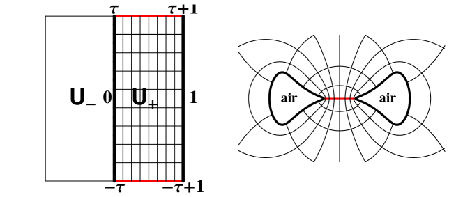
Figure 5: Mathematical plane (left) and the physical domain (right). Conformal map, $z(u)$, maps ${\sf U}_{+}$ to the oil-domain $\mathbb{C}\setminus{\sf D}$. We can see that the grid lines in ${\sf U}_{+}$ are distorted in $\mathbb{C}\setminus{\sf D}$ by the mapping. The thick lines at ${\rm Re}(u)=0$ and ${\rm Re}(u)=1$ correspond to the interfaces. The red line at the top (bottom) maps to the critical region.

A Riemann surface describing two bubbles, has the topology of a torus. The torus is modelled as the complex plane modulo the periods $2\omega_{1}$ and $2\omega_{2}$. The anti-holomorphic involution is chosen as $f(u)=-u$, and requires $\omega_{1}$ to be real and $\omega_{2}$ to be imaginary Why . Choosing a proper scale we set $\omega_{1}=1$ and $\omega_{2}=\tau$, where $\tau$ is an imaginary number—the modulus of the torus—which changes with time. We take the fundamental domain of $\sf U$ as $-1<{\rm Re}(u)\leq 1$ and $-|\tau|<{\rm Im}(u)\leq|\tau|$ with the opposite edges identified as in Fig. 5. The fixed points of the involution are the lines: ${\rm Re}(u)=0$ and ${\rm Re}(u)=1$. Each corresponds to each boundary of the bubbles.

We will follow Refrs. Ri ; Why to construct a map $z(u)$. For simplicity we discuss only the quadrature domains, where there is no log-singularity in $z(u)$. The map can be written in terms of the Weierstrass zeta function $\zeta(u)$: a quasi-periodic function satisfying,

$$\zeta(u+2\omega_{i})=\zeta(u)+2\eta_{i},\quad\eta_{i}\equiv\zeta(\omega_{i}),\quad i=1,2.$$

with a simple pole of residue $1$ at the origin $\zeta(u)\sim u^{-1}$.

The map $z(u)$ reads

$$z(u)=\alpha_{0}\zeta(u-u_{0})+\beta+\sum_{j=1}^{K}\alpha_{j}\zeta(u-u_{j})$$ (15)

where $u_{0}\in U_{+}$ and $u_{j}\in U_{-}$ for $j=1,\cdots,K$. The condition $0=\sum_{j=0}^{K}\alpha_{j}$ ensures the periodicity of the map. It reduces the total number of complex variables (excluding the modulus $\tau$) to $2K+2$. The constants of motion are computed from (13):

$$\mu_{j}=\overline{\alpha_{j}}\partial z(u^{*}_{j})\quad\mbox{and}\quad q_{j}=z(u^{*}_{j}),\quad(j=1,\cdots,K)$$ (16)

and from (14):

$$q_{0}=z(u^{*}_{0})\quad\mbox{and}\quad\mu_{0}=\overline{\alpha_{0}}\partial z(u^{*}_{0})=t+const.$$ (17)

Hence the total number of equations is $2K+2$ as well.

The modulus $\tau$ is chosen to ensure the equal pressure between the two bubbles: $0=\frac{1}{2}\partial_{t}\oint_{\bf b}S(z)\,dz$, where ${\bf b}$ is a cycle traversing the two bubbles. Integrating this equation we obtain another constant of motion, $\Pi$:

$$\Pi=\frac{1}{2}\oint_{\bf b}S(z)\,dz.$$ (18)

Before a break-off the cycle $\bf b$ does not exist, and at the break-off it contracts to a point. Therefore $\Pi$ must be zero for a break-off: $\Pi=0$, which provides the equation to determined the modulus. In terms of our conformal map:

$$0=\Pi=\sum_{j=0}^{K}\eta_{1}(\alpha_{j}\overline{q}_{j}-u_{j}\overline{\mu}_{j}-\overline{u}_{j}\mu_{j})-\sum_{j,k=0}^{K}\overline{\alpha}_{j}\alpha_{k}\left(\frac{\wp^{\prime}(\overline{u}_{j}+u_{k})}{2}+\zeta(\overline{u}_{j}+u_{k})\wp(\overline{u}_{j}+u_{k})\right),$$ (19)

where $\tau$ is implicit in all the elliptic functions.

In the conventional set-up where air is injected into bubbles, a smooth merging occurs only for a fine-tuned initial condition which satisfies $\Pi=0$ (19). If $\Pi\neq 0$, one bubble develops a singular cusp before the merging. After this moment the problem without surface tension becomes ill-posed, and requires a regularization.

IV Break-off

To illustrate a break-off we restrict ourselves to a left-right symmetric case. In this case a bubble will be broken into two symmetrical bubbles: one is a mirror reflection of the other. The pressure is also symmetric, and $\Pi$ is vanishing automatically.

It is convenient to follow the reversed evolution, that is, to consider a merger rather than a break-off. At the merger the period ($2\omega_{2}$) blows up; a rectangular fundamental domain becomes an infinitely long channel—a cylinder; the doubly periodic function $\zeta(u)$ degenerates into a periodic function with period $2\omega_{1}=2$. Accordingly, the (imaginary) modulus $\tau$ gets infinitely large. Therefore, a convenient small parameter for an expansion is $e^{i\pi\tau}<1$ (the nome of the Jacobi theta function) which becomes zero when a merging occurs. Here we only consider the situation up to the merging point, not after: $t<0$.

The area near the merger corresponds to the domain near the top of the rectangle. In $u$-coordinate this region is pushed away to the infinity as $e^{i\pi\tau}\to 0$. A new coordinate $\tilde{u}=u-\tau$ whose origin resides at the top of the rectangle is proper. We use the expansion in small $e^{i\pi\tau}$:

$$\zeta(u)=\zeta(\tilde{u}+\tau)=\frac{\pi^{2}}{12}(1-24e^{2i\pi\tau})\tilde{u}+2\pi e^{i\pi\tau}\,\sin\pi\tilde{u}+2\pi e^{2i\pi\tau}\sin 2\pi\tilde{u}+\cdots,$$

up to $\tilde{u}$-independent constants. The map (15) expands:

$$z(\tilde{u}+\tau) = C+e^{i\pi\tau}\left(A_{1}\sin\pi\tilde{u}+B_{1}\cos\pi\tilde{u}\right)+e^{2i\pi\tau}\left(A_{2}\sin 2\pi\tilde{u}+B_{2}\cos 2\pi\tilde{u}\right)+\cdots,$$ (20)

where

$$A_{n}=2\pi\sum_{k=0}^{K}\alpha_{k}\cos n\pi u_{k},\quad B_{n}=-2\pi\sum_{k=0}^{K}\alpha_{k}\sin n\pi u_{k},\quad n=1,2.$$

For a generic choice of the parameters shape of the interface is not physically acceptable: it may contain self-intersecting interface.

A particularly simple configuration occurs by further imposing up-down symmetry. (A break-off with no up-down symmetry is shown in Fig. 6.) The full symmetry (up-down and left-right) may be realized by setting (i) $u_{0}=\frac{1}{2}$, (ii) the points $u_{k}$ in ${\sf U}_{-}$ are all on the line ${\rm Re}(u)=-\frac{1}{2}$ symmetrically with respect to the real axis, (iii) the residues $\alpha_{k}$’s are all real, and the residues at poles $u_{k}$ and $\bar{u}_{k}$ are equal, iv) the merging point is at the origin: $z(\frac{1}{2}+\tau)=0$. Then we get $C=0$ and $A_{1}=B_{2}=0$.

Within this configuration let us solve the string equation (7), which is modified into the following form using (10):

$$\partial z(u)\partial_{t}\overline{z}(-u)-\partial_{t}z(u)\partial\overline{z}(-u)=i\partial\phi(u).$$ (21)

One use the expansion of $z(u)$ (20) to obtain the l.h.s. of the above equation (21):

$$(l.h.s.)\sim 2\pi e^{i\pi\tau}\,\frac{d\,e^{2i\pi\tau}}{dt}\cos\pi\tilde{u},$$ (22)

where the two remaining constants, $A_{2}$ and $B_{1}$, are reduced to 1 by a rescaling of coordinates.

To obtain the r.h.s. of (21) we must find a meromorphic function $\phi(u)$ that has vanishing imaginary part along the lines ${\rm Re}(u)=0$ and ${\rm Re}(u)=1$ and has the asymptotic behavior of $\phi(z)=i\log(u-u_{0})\sim-i\log z$ near infinity. One can construct such function $\phi(z)$ using the Weierstrass sigma function $\sigma(u)$:

$$\phi(u)=i\log\frac{\sigma(u-u_{0})}{\sigma(u-u^{*}_{0})}+2i\,\eta_{1}{\rm Re}(u_{0})\,u.$$

The first term renders ${\rm Im}[\phi(u)]$ constant along each line ${\rm Re}(u)=0$ and ${\rm Re}(u)=1$, then the second term shifts it to zero for both lines. In the critical regime one can also expand $\phi(u)$ to produce:

$$(r.h.s.)=i\partial\phi(u)\sim 4\pi\,e^{i\pi\tau}\cos\pi\tilde{u}.$$

Combined with the l.h.s. (22) we obtain $\frac{d\,e^{2i\pi\tau}}{dt}=const.$, or equivalently,

$$e^{i\pi\tau}\sim\sqrt{|t|}$$

with $t=0$ being the merging point ($t$ is negative before merging).

The evolution of the interface is described at the leading order:

$$(x,y)\sim(\sqrt{|t|}\ \cosh\pi s,\;|t|\sinh 2\pi s)$$

with $s\in{\mathbb{R}}$ parametrizing the interface. Alternatively

$$y=x^{2}F\left(\frac{\sqrt{|t|}}{x}\right),\quad F(\xi)=\sqrt{1-\xi^{2}}.$$

This is the simplest and the most generic (4,2)-class of the break-off.

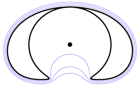
Figure 6: Up-down symmetry is broken. Thick line is the boundary. Thin lines are equi-pressure lines. The dot is one of the stagnation points. There is a merger in the upper part. Another merger in the bottom is imminent, whereupon the bubble will form a ring-type domain.

V Critical regime

While breaking-off the shape of the interface near the break-off point does not depend on the details of the rest of the bubble: locally, the breaking interface is universal. We will call this regime critical.

In the critical regime, different scales separate. It is convenient to define the scales in the complex plane of $\phi$—the complex counterpart of pressure—which can be put to zero at the the tips. As we did in the previous section, it is convenient to think about break-off in a reversed time. Then the process appears as a merger.

A critical regime is the image of a small domain containing the point $\phi=0$. We saw that at $\phi\sim e^{i\pi\tau}$ we see the details of the tips of the merging bubbles and details of the neck after they merge. At $1\gg\phi\gg e^{i\pi\tau}$, however, the details of the neck and the tip cannot be seen, and the details of the remote part of the bubble can not be seen either. At this scale we see only the asymptote of the neck $y^{q}\sim x^{p}$. Finally, $\phi=O(1)$ corresponds to the rest of the body of the bubble. The scale $e^{i\pi\tau}$ changes with time and eventually disappears at the critical point. In that limit, the shape is scale invariant as in Fig. 4. Two even integers $p$ and $q$ characterize the critical regime. They are sufficient to determine the scaling functions.

We find solutions only for $(p,q)=(4n,2)$, where $n$ is an integer. A similar analysis has been carried out for cusp-like singularity of Hele-Shaw flow in Teo2 .

V.1 (4,2)-break-off

We start from the most generic (4,2)-class, $\tilde{y}\propto A_{\pm}\tilde{x}^{2}$, where the asymptotes may differ at both sides of the $x$ axis, $A_{+}\neq-A_{-}$. More degenerate $(4n,2)$ will be addressed later.

After break-off we expect two distinct tips, located respectively at $x=u_{1}$ and $x=u_{2}$. Assuming these tips are smooth, we have an expansion: $\tilde{x}-u_{i}\propto\tilde{y}^{2}+O(\tilde{y}^{3})$, which leads to branch cut singularities at $u_{1}$ and $u_{2}$. Together with the $(4,2)$ asymptote we are led to the following form for the curve:

$$\tilde{y}(\tilde{x})=a(\tilde{x}-b)\sqrt{(\tilde{x}-u_{1})(\tilde{x}-u_{2})}+c\tilde{x}^{2}+d\tilde{x}+e,$$ (23)

with $b$, $u_{1}$, $u_{2}$, $d$, and $e$ vanishing at $t=0$.

The potential $\phi(\tilde{x})$ must have the same branch points as the curve, it must behave as $\tilde{x}$ at large (but not too large) $\tilde{x}$, and is real on the curve (when $\tilde{x}$ is a real coordinate of the curve). These requirements determine the potential:

$$\phi=-\sqrt{(\tilde{x}-u_{1})(\tilde{x}-u_{2})}-\gamma\tilde{x}.$$ (24)

The overall normalization can be chosen by a proper rescaling of time $t$, the coefficient $c$ controls the up-down asymmetry of the shape shown in the asymptote $\tilde{y}\propto(\pm a+c)\tilde{x}^{2}$, the coefficients $e$ and $\gamma$ control the up-down asymmetry of the velocity. In fact they will be connected by $e=\gamma t$.

Putting this ansatz into the evolution equation (9): $\partial_{t}\tilde{y}(\tilde{x})=-\partial_{\tilde{x}}\phi(\tilde{x})$, we see that the regular polynomial part of $\tilde{y}$ and its singular part consisting of the square root are decoupled. The solution for the polynomial part set $d=0$, and $c$ as a constant, and confirms that $e=\gamma t$.

In order to match the singular parts of $\partial_{y}\tilde{y}(\tilde{x})$ and $-\partial_{\tilde{x}}\phi(\tilde{x})$, it is sufficient to match their large $\tilde{x}$-expansions. $\tilde{y}$ expands as:

$$a\Big{[}\tilde{x}^{2}-\Big{(}b+\frac{u_{1}+u_{2}}{2}\Big{)}\tilde{x}+\frac{4(u_{1}+u_{2})b-(u_{1}-u_{2})^{2}}{8}+\frac{(2b-u_{1}-u_{2})(u_{1}-u_{2})^{2}}{16\,\tilde{x}}+\cdots\Big{]},$$ (25)

while the expansion of the singular part of $-\partial_{\tilde{x}}\phi(\tilde{x})$ is: $1+{\cal O}(\tilde{x}^{-2})$. Comparing, we conclude that the coefficients of the $\tilde{x}^{2},\,\tilde{x}$ and $\tilde{x}^{-1}$ terms in (25) are constants and that the constant term is proportional to time. The constants must be chosen such that the shape is $\tilde{y}=(\pm a+c)\tilde{x}^{2}$ at time $t=0$. This is equivalent to setting the parameter $\Pi$ in (19) to zero. We obtain $u_{1}=-u_{2}=\sqrt{\frac{2|t|}{a}}$ and $b=0$. Summing up we find an evolving curve (we write it in a self-similar form):

$$\tilde{y}=\tilde{x}^{2}\left(a\sqrt{1+\frac{2t}{a\tilde{x}^{2}}}+c+\gamma\frac{t}{\tilde{x}^{2}}\right).\quad\mbox{at}\quad t<0$$ (26)

Now we turn our attention to the flow after merging (before the break-off). It is simpler since it doesn’t involve any singularities. When the branch points meet to become a double point the curve degenerates. The potential becomes $\phi(\tilde{x})=\pm\tilde{x}-\gamma\tilde{x}.$ A similar procedure yields the following curve as the one before the break-off:

$$\tilde{y}=\tilde{x}^{2}\left(\pm a\left(1+\frac{t}{a\tilde{x}^{2}}\right)+c+\gamma\frac{t}{\tilde{x}^{2}}\right).\quad\mbox{at}\quad t>0$$ (27)

Equations (26) and (27) form our prediction of the self-similar dynamics for the generic $(4,2)$-break-off.

V.2 $(4n,2)$-break-offs

There is a larger class of solutions of the Eq. 9 for the same form of the potential (24). They belong to the $(4n,2)$ class. Below we only consider the curve with up-down symmetry: symmetric w.r.t. $x$-axis. In this case the curve and the potential read:

$$\tilde{y}=P(\tilde{x})\sqrt{(\tilde{x}-u_{1})(\tilde{x}-u_{2})},\quad\phi=-\sqrt{(\tilde{x}-u_{1})(\tilde{x}-u_{2})},$$ (28)

where $P(x)$ is a polynomial of degree $2n-1$. Its zeros are called the double points. Eq. 28 represents a degenerate hyperelliptic curve, where all but one branch cut shrink to double points. Double points and the branch points $u_{1}$ and $u_{2}$ move in time as determined by (9).

A formally identical problem appeared in the study of dispersionless integrable hierarchies kodama ; Kono . Below we adapt some of the results. The idea is based on the following observation: the large $\tilde{x}$-expansion of $\tilde{y}$ in (28) starts with $2n$ terms of positive powers in $\tilde{x}$, while the expansion of $\partial\phi$ starts from the constant $-1$ and skips the $\tilde{x}^{-1}$ term. These expansions match only if the coefficients of the positive powers of $\tilde{y}$ do not change in time, while the zeroth order term of the expansion of $\tilde{y}$ is equal to $t$, and the coefficient in front of $\tilde{x}^{-1}$ is a constant. Once these terms are matched the negative powers match automatically. In the previous section we saw how it works on the simplest $(4,2)$ example.

The functions ${H}_{k}(\tilde{x})$, defined below, form a useful basis of functions with proper analytical behavior: these functions have the same branch points as $\tilde{\phi}(\tilde{x})$, behave as $\tilde{x}^{k}$ at large $\tilde{x}$, and lack all other positive powers in large $\tilde{x}$-expansion: ${H}_{k}(\tilde{x})=\tilde{x}^{k}+O(1)$ for $k=1,2,\cdots$. These properties uniquely determine them to be given by the formula:

$${H}_{k}(\tilde{x}) = \left(\frac{\tilde{x}^{k}}{\sqrt{(\tilde{x}-v)^{2}-r^{2}}}\right)_{+}\sqrt{(\tilde{x}-v)^{2}-r^{2}}$$

$$= \tilde{x}^{k}-\frac{{R}_{k+1}}{r}-\frac{{V}_{k+1}}{\tilde{x}}+\cdots,$$

where the subscript $+$ denotes the polynomial part of the large $\tilde{x}$ expansion. We set

$$v=\frac{u_{1}+u_{2}}{2},\quad r=\frac{u_{1}-u_{2}}{2}.$$ (30)

The two next leading coefficients ${R}_{k}$ and $V_{k}$ are homogeneous polynomials in $r$ and $v$ of degree $k$ which may be expressed through Legendre polynomials as

$${R}_{k+1}=(-i)^{k}\rho^{k+1}\cosh\varphi\,P_{k}(i\sinh\varphi)$$ (31)

$${V}_{k+1}=(-i)^{k-1}\rho^{k+1}\frac{\cosh^{2}\varphi}{k+1}\,P^{\prime}_{k}(i\sinh\varphi),$$

where

$$\rho^{2}=r^{2}-v^{2},\quad~{}\sinh\varphi=\frac{v}{\rho},\quad\cosh\varphi=\frac{r}{\rho}.$$

A general solution is written as a superposition of ${H}_{k}$ with coefficients $t_{k}$’s (that will turn out to be time-independent):

$$\tilde{y}(\tilde{x})=\sum_{k=1}^{2n}(k+1)t_{k}{H}_{k}(\tilde{x}).$$ (32)

The coefficients are the deformation parameters. The differential form of these equation is:

$$\partial_{t_{k}}\tilde{y}=\partial_{\tilde{x}}H_{k+1}.$$

Matching the leading powers of the expansion (V.2) we get

$$\partial_{t}t_{k}=0,\quad\mbox{for}\quad k=1,\cdots,2n$$

$$t\,r=-\sum_{k=1}^{2n}(k+1)t_{k}{{R}_{k+1}},$$ (33)

$$\Pi=-\sum_{k=1}^{2n}(k+1)t_{k}{V}_{k+1},$$

where $\Pi$ is a constant of integration. The $2n+2$ conditions (33) determine $2n$ coefficients of the polynomial (28) and 2 branch points. Thus solving these algebraic equations is equivalent to solving the Hele-Shaw problem near the break-off. The last pair of these equations is called the hodograph relation.

The constant, $\Pi$, is the coefficient in front of $\tilde{x}^{-1}$ term of the expansion of $\tilde{y}$, and is exactly the integral (18) over the ${\bf b}$-cycle of the curve $\tilde{y}(\tilde{x})$ (28) - the integral along the cycle encircling the two branch points. It must vanish for a break-off.

A particularly simple case occurs at $v=0$ when the curve is left-right symmetric. Then $\Pi=0$, and hodograph equation (33) becomes:

$$t=\sum_{k=1}^{n}(2k+1)(-1)^{k+1}\begin{pmatrix}-\frac{1}{2}\\ k\end{pmatrix}\,t_{2k}\,r^{2k},$$

which determines the time dependence of $r$.

V.3 Various break-offs : self-similarity

Self-similar solutions are of a particular interest. There the evolution of the curve can be viewed as a scaling transformation of the coordinate $\tilde{y}$ and $\tilde{x}$. They occur when all the deformation parameter are set to zero except one from even order which we normalize as $t_{2n}=\frac{1}{2n+1}$. As a consequence of the merging condition $\Pi=0$ we have $v=0$, and $r$ remains as the only scale.

$$\tilde{y}(\tilde{x}) = {H}_{2n}(\tilde{x})=\left(\frac{\tilde{x}^{2n}}{\sqrt{\tilde{x}^{2}-r^{2}}}\right)_{+}\sqrt{\tilde{x}^{2}-r^{2}},$$ (34)

The curve enjoys an explicit formula in terms of the Chebyshev polynomial of the second kind: $U_{m}(\cosh\theta)=\frac{\sinh(m+1)\theta}{\sinh\theta}$.

$${H}_{2k}(\tilde{x}) = 2\sinh\theta\,\Big{(}\frac{r}{2}\Big{)}^{2k}\sum_{j=0}^{k-1}\begin{pmatrix}2k\\ j\end{pmatrix}\,U_{2k-2j-1}(\cosh\theta).\quad\mbox{where}\quad\cosh\theta\equiv\frac{\tilde{x}}{r}$$

The hodograph Eq. 33 degenerates into $t\,r=\left.-{R}_{2n+1}\right|_{v=0}=(-1)^{n+1}\begin{pmatrix}-\frac{1}{2}\\ n\end{pmatrix}\,r^{2n+1}$ and yields

$$r\propto|t|^{1/2n}.$$

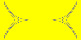
Figure 7: (8,2)-break-off at three successive time slices. Only $t_{4}$ is turned on. The curve is $\tilde{y}=\tilde{x}(\tilde{x}^{2}-\frac{r^{2}}{2})\sqrt{\tilde{x}^{2}-r^{2}}$. It shows more singular behavior than the (4,2)-break-off: $r\sim|t|^{1/4}$.

As an example the Fig. 7 illustrates ($8,2$)-break-off.

Another interesting case occurs at $u_{2}\to\infty$ while $u_{1}$ remains finite. In this case the distance between the bubbles is so large that one sees only a tip of one bubble. This case has been studied in Teo2 .

VI Hele-Shaw flows and dispersionless integrable hierarchy

Here we summarize features of the AKNS hierarchy and its relation to break-offs in the Hele-Shaw flow. We will show that the flow is identical to the evolution of the spectral curve appearing in the dispersionless AKNS (dAKNS) hierarchy. We start by reviewing the AKNS hierarchy book ; book2 .

VI.1 AKNS hierarchy

The AKNS hierarchy is an infinite set of non-linear differential equations written for two functions $r$ and $v$, which depend on time $t_{0}$ and an infinite set of deformation parameters (flows) $t_{k}$’s . An efficient way of defining the hierarchy requires the definitions of a few objects, first.

The first is the Lax operator $L$, a $2\times 2$ matrix consisting of a differential operator $\hbar\partial_{t_{0}}$ (Later we will consider the limit, $\hbar\to 0$, so we keep $\hbar$ in some of the formulae in this section), boost

$$L=\hbar\partial_{t_{0}}+U,\quad U=\frac{1}{2}\left(\begin{array}[]{cc}iv&r\\ r&-iv\end{array}\right).$$

The second object is the resolvent $Q(\tilde{x})$, defined as the diagonal component of the Green function: $Q(\tilde{x})=i\langle t_{0}|(L-i\tilde{x}\frac{\sigma_{3}}{2})^{-1}|t_{0}\rangle$, which is formally expanded in the spectral parameter $\tilde{x}$ as

$$Q(\tilde{x})=\sum_{k=1}^{\infty}Q_{k}\tilde{x}^{-k},\quad\quad\Big{(}Q_{0}=i\frac{\sigma_{3}}{2}\Big{)}$$

where the series of $2\times 2$ matrices $Q_{k}$’s are determined from the commutation relation,

$$\left[Q(\tilde{x}),L-i\tilde{x}\frac{\sigma_{3}}{2}\right]=0,$$ (35)

which, being expanded in powers of $\tilde{x}$, yield the recurrence relation for $Q_{k}$:

$$\frac{i}{2}[\sigma_{3},Q_{k+1}]=\hbar\partial_{t_{0}}Q_{k}+[U,Q_{k}].$$ (36)

The first few terms are given as

$$Q_{1} = -r\frac{\sigma_{1}}{2},$$

$$Q_{2} = -rv\frac{\sigma_{1}}{2}-r^{\prime}\frac{\sigma_{2}}{2}+i\frac{r^{2}}{2}\frac{\sigma_{3}}{2},$$

$$Q_{3} = -(\frac{1}{2}r^{3}+v^{2}r-r^{\prime\prime})\frac{\sigma_{1}}{2}-(2r^{\prime}v+rv^{\prime})\frac{\sigma_{2}}{2}+ir^{2}v\frac{\sigma_{3}}{2},$$

where “$~{}^{\prime}~{}$” means the time derivative: $\hbar\partial_{t_{0}}$. For general $k$, $Q_{k}$ is a polynomial of degree $k$ in $r$ and $v$, and their time derivatives. It follows, from the above definition of $Q_{1}$, that the equation $\hbar\partial_{t_{0}}L=[Q_{1}-iv\frac{\sigma_{3}}{2},\,L]$ holds trivially.

The dependence on the deformation parameters can be introduced accordingly. Including the time in the set of parameters we now define a hierarchy of flows as boost

$$\hbar\partial_{t_{k}}L=[Q_{k+1}-i\hbar\partial_{t_{k}}\beta\frac{\sigma_{3}}{2},L],\quad k=0,1,2,\cdots.$$ (37)

where $\beta\equiv\frac{1}{\hbar}\int v\,dt_{0}$. Eq. 35 ensures compatibility of the equations: the flows commute.

The first two flow equations are given by

$$t_{1} : \pm i\hbar\partial_{t_{1}}(re^{\pm i\beta})=(re^{\pm i\beta})^{\prime\prime}-\frac{r^{2}}{2}(re^{\pm i\beta})$$ (38)

$$t_{2} : \begin{cases}\hbar\partial_{t_{2}}r=\frac{3}{2}r^{2}r^{\prime}+3r^{\prime}v^{2}+3rvv^{\prime}-r^{\prime\prime\prime}\\ \hbar\partial_{t_{2}}\beta=\frac{3}{2}r^{2}v+v^{3}-3\frac{r^{\prime}}{r}v^{\prime}-3\frac{r^{\prime\prime}}{r}v-v^{\prime\prime}\end{cases}$$

The recursion relations (36) and the flow equations (37) are more explicitly written in terms of the components of $Q_{k}$,

$$Q_{k}\equiv-{\cal R}_{k}\frac{\sigma_{1}}{2}+\Theta_{k}\frac{\sigma_{2}}{2}+i{\cal V}_{k}\frac{\sigma_{3}}{2}.$$

They are: $r\Theta_{k}=-{\cal V}^{\prime}_{k}$, and

$${\cal R}_{k+1}=r{\cal V}_{k}+v{\cal R}_{k}-\left(\frac{{\cal V}^{\prime}_{k}}{r}\right)^{\prime},$$ (39)

$${\cal V}^{\prime}_{k+1}=v{\cal V}^{\prime}_{k}+r{\cal R}^{\prime}_{k},$$ (40)

and the flow equations (37):

$$\partial_{t_{k}}r=\frac{{\cal V}^{\prime}_{k+2}}{r},\quad\partial_{t_{k}}v=\left(\frac{{\cal R}_{k+2}}{r}\right)^{\prime}.$$ (41)

It follows that the flows can be written in an integrated form KMS

$$0 = \sum_{k=0}(k+1)t_{k}{\cal R}_{k+1}$$ (42)

$$-\Pi = \sum_{k=0}(k+1)t_{k}{\cal V}_{k+1}$$

with a constant $\Pi$. Alternatively, this hodograph-type relations (42) may be used as a definition of the hierarchy. The reader may notice that the structure of these equations is similar to the hodograph equations in (33).

There are several known reductions of AKNS hierarchy.

• NLS: When $r$ is purely imaginary, the first flow equation of the hierarchy is non-linear Schroedinger equation.

  $$0=i\dot{\psi}+\psi^{\prime\prime}+\frac{|\psi|^{2}}{2}\psi,\quad\psi=\pm ire^{-i\beta},\quad(\mbox{NLS equation})$$

  This reduction seems to be irrelevant for the Hele-Shaw problem. Other reductions are relevant.

• mKdV: When $v=0$ and $\kappa=\pm ir$. The even flows constitute mKdV hierarchy. The first equation of the hierarchy is the $t_{2}$-flow:

  $$0=\dot{\kappa}+\frac{3}{2}\kappa^{2}\kappa^{\prime}+\kappa^{\prime\prime\prime}.\quad\quad~{}(\mbox{mKdV equation})$$

  where “ $\dot{}$ ” stands for $\hbar\partial_{t_{2}}$.

• N-AKNS: It occurs if all the deformation parameters vanish except: $t_{N}=\frac{1}{N+1}$. The first interesting case occurs at $N=2$. In this case (42) reads

  $$\frac{r^{3}}{2}+v^{2}r-r^{\prime\prime}+t_{0}r=0$$

  $$r^{2}v+\Pi=0$$

  which, after elimination of $v$ yields the (modified) Painlevé II equation

  $$r^{\prime\prime}=\frac{r^{3}}{2}+\frac{\Pi^{2}}{r^{3}}+t_{0}r.$$ (43)

VI.2 Linear problem and $M$ operator

The flow equations appear as a result of compatibility of the spectral problems:

$$L\Psi=i\tilde{x}\frac{\sigma_{3}}{2}\Psi,$$ (44)

and,

$$\hbar\partial_{t_{k}}\Psi=\Big{(}{\cal H}_{k+1}(\tilde{x})-i\hbar\partial_{t_{k}}\beta\frac{\sigma_{3}}{2}\Big{)}\Psi,$$ (45)

where ${\cal H}_{k}(\tilde{x})=Q_{0}\tilde{x}^{k}+Q_{1}\tilde{x}^{k-1}+\cdots+Q_{k}$. boost

Another important object of the hierarchy is the $M$-operator defined as

$$M(\tilde{x})\Psi=\partial_{\tilde{x}}\Psi.$$ (46)

Its relation to flows follows from compatibility of the above definition with the Lax equations (44,45)

$$M(\tilde{x})=\sum(k+1)t_{k}\Big{(}{\cal H}_{k}(\tilde{x})-i\hbar\partial_{t_{k-1}}\beta\frac{\sigma_{3}}{2}\Big{)}.$$ (47)

The proof is standard in the theory of integrable hierarchy. We sketch it in the Appendix D.

The relation expressing the compatibility of (44) and (46):

$$[M(\tilde{x}),L-i\tilde{x}\frac{\sigma_{3}}{2}]=-i\frac{\sigma_{3}}{2},$$ (48)

is sometimes referred to as the string equation. The $M$-operator reflects homogeneous properties of the wave function $\Psi$ with respect to the scaling transformations: $t_{k}\to\lambda^{k+1}t_{k}$, and $(\tilde{x},r,v)\to(\frac{\tilde{x}}{\lambda},\frac{r}{\lambda},\frac{v}{\lambda})$.

VI.3 Dispersionless limit and genus-0 Whitham equations

The Hele-Shaw problem appears as a dispersionless limit of the hierarchy as $\hbar\to 0$.

Let us pursue the limit on a formal level. As is typical for a semiclassical approximations the wave function has the form

$$\Psi\sim e^{-\frac{1}{\hbar}{\cal A}},$$ (49)

where the “momentum,” $\phi=2i\partial_{t_{0}}{\cal A}$, obeys the spectral equation

$$\det\left(\frac{i}{2}\phi+U-i\tilde{x}\frac{\sigma_{3}}{2}\right)=0.$$

The latter gives a relation between the “momentum” $\phi$ and the spectral parameter

$$\phi^{2}(\tilde{x})=(\tilde{x}-v)^{2}-r^{2},$$

and determines a spectral surface—a Riemann surface where the wave function is univalent.

Accordingly, the commutator in (48) is replaced by a Poisson bracket. If $\tilde{y}(\tilde{x})$ is an eigenvalue of the operator $M(\tilde{x})$, treated as a function on the spectral surface, the pair $\tilde{y}(\tilde{x}(\phi))$ and $\tilde{x}(\phi)$ obey the dispersionless string equation

$$\{\tilde{y},\tilde{x}\}=1.$$

An alternative form of this equation follows from (46),

$$\partial_{t_{0}}y=-\partial_{\tilde{x}}\phi$$ (50)

where the time derivative is taken at a fixed $\tilde{x}$.

The dispersionless limit of Eqs. 38,39,43 is easy. One simply drops the time derivative there. In this limit the objects of AKNS hierarchy converge to the objects discussed in the previous section V.2.

$${\cal R}_{k}\to R_{k},$$

$${\cal V}_{k}\to V_{k},$$

$$\sqrt{\det|{\cal H}_{k}-i\frac{{\cal R}_{k+1}}{r}\frac{\sigma_{3}}{2}|}\to H_{k}.$$

Under this identification (42) become (33), and the Hele-Shaw dynamics is seen to be governed by the dispersionless AKNS hierarchy. The dispersionless limit can be also understood as genus-0 Whitham equations. We briefly discuss it below. For a comprehensive description of Whitham theory see Whitham .

Integrable equations have special solutions known as finite-gap solutions. They are quasi-periodic in times. For these cases, the wave-function $\Psi$ as a function of the spectral parameter $\tilde{x}$ is multi-valued. It is a univalent on a spectral surface. The case when $r$ and $v$ do not depend on time $t_{0}$ is the simplest example. The period of this solution is infinite, but the wave function of this solution oscillates with a period $\sim\hbar^{-1}$. Then the formula (49) gives an exact solution. The genus of the spectral surface is zero.

A class of non-periodic solutions may be obtained from periodic solutions under assumption that periods (the moduli) of the solution depend on time but change slowly, such that they do not change much at the time of the order to $\hbar$. Constructions of slowly modulated solutions is the subject of Whitham theory.

Modulation of genus-0 solutions is simplest. In order to obtain it one simply drops the time derivatives in most equations as it has been discussed above. By doing so we obtain the same equations as obtained for the break-off in the previous section.

VI.4 Hele-Shaw flow and dispersionless limit of integrable hierarchy

As we have seen, the dispersionless limit of AKNS hierarchy and equations for the Hele-Shaw flow close to a break-off/merging are identical. This is not an accident. In KM-WWZ an equivalence between Hele-Shaw and the universal Whitham hierarchy has been established on general grounds.

The relation between integrable hierarchies and Hele-Shaw flows can be summarized as follows: in the limit $\hbar\to 0$

• the eigenvalues of the Lax operator become different branches of the potential $L\to\phi(\tilde{x})$;

• the operator $M$ becomes the height function $M\to\tilde{y}(\tilde{x})$;

• the real section of the spectral curve $\tilde{y}(\tilde{x})$ when $\tilde{y}=y,\,\tilde{x}=x$ is identified with the form of the interface;

• Eq. 48 converts to D’Arcy’s law written in the form (8);

• The integrable hierarchy describe the response of the interface to a variation of deformation parameters.

VII Hele-Shaw problem as a singular limit of dispersive non-linear waves

A relation between the Hele-Shaw problem and the dispersionless limit of integrable equations reveals the nature of fingering instabilities and singularities of the Hele-Shaw problem. It is known for a long time that the dispersionless limit $\hbar\to 0$ of dispersive non-linear waves is singular singular . Despite the fact that the integrable equations are well defined at all times, the $\hbar\to 0$ limit of some—the most relevant—solutions cannot be taken after some finite time of evolution. These solutions develop singular features at small scales of the order $\hbar$ and have no meaning at $\hbar=0$. These singularities appear in non-linear waves as shock waves. In Hele-Shaw flows where the surface tension is omitted they appear as cusp-like singularities.

Some solutions, however, do not lead to a singularity. One of them has been considered in this paper. An inevitable break-off of the extracting process in Fig. 2, although singular, is well defined at all time even in the limit of zero-surface tension.

However, an injection process, unless it is fine-tuned to satisfy $\Pi=0$, leads to cusp-singularities.

We can summarize this on a simple example of Painléve II Eq. 43

$$\hbar^{2}\partial_{t}^{2}r=\frac{r^{3}}{2}+\frac{\Pi^{2}}{r^{3}}+t_{0}r.$$ (51)

As we have mentioned the $\hbar\to 0$ limit of this equation,

$$0=\frac{r^{3}}{2}+\frac{\Pi^{2}}{r^{3}}+t_{0}r,$$ (52)

describes the critical regime when all deformation parameters $t_{k}$ vanish for $k>2$. In this limit $r$ and $v$ have a simple interpretation: $r$ is a the distance between two tips, $v=-\frac{\Pi}{r^{2}}$ is a measure of asymmetry of the bubbles (Fig. 8). When $\Pi=0$ the bubbles merge according to the law $r=\sqrt{-2t_{0}}$. When $\Pi\neq 0$, however, Eq. 52 happens to have four real solutions. The graph of $r(t_{0})$ overhangs at some time $t^{*}=-\frac{3\Pi^{2/3}}{2^{4/3}}$ with $r(t^{*})=2^{1/3}\Pi^{1/3}$ as in Fig. 9. At this point the tip of one droplet develops a (2,3) cusp singularity $y^{2}\sim x^{3}$ as shown in Fig. 8. Equation (52), as well as the original un-regularized D’Arcy law (9), have no sense beyond this point.

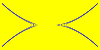
Figure 8: (4,2)-break-off with nonzero $\Pi$. One of the tip develops a (2,3)-cusp before merging. Evolution beyond this point requires a regularization of the cusp-singularity.

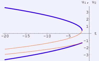
Figure 9: Trajectory of the branch points $u_{1}$ and $u_{2}$ from solving the dispersionless limit of Painlevé II equation (52). Blue (thick) line is the physical solution and the red (thin) line is the unphysical solution. Being continued through the cusp, the solution becomes multi-valued and therefore unphysical.

However, the Painlevé II Eq. 51 is well defined at any time. The approximation of simply dropping the dispersion term $\hbar^{2}\partial_{t}^{2}r$ is invalid. The reason is simple: an initially smooth function such as $r(t)$ will get sharper, such that the dispersion is no longer small. In fact the approximation becomes invalid some time before the overhang occurs. This phenomena is known in the theory of non-linear wave as a gradient catastrophe.

The relation between the integrable equations and the Hele-Shaw problem raises a natural question. Can the Hele-Shaw problem be extended beyond $\hbar\to 0$ limit? Can the parameter $\hbar$ be used to regularize singularities in a meaningful physical way? These questions will be the subject of future study.

VIII Conclusion

We have analyzed the universal shapes of bubbles in a Hele-Shaw cell at break-off. These are given by the Eq. 26. At the pinch-off point the shapes are universal and self-similar: their evolution is reduced to a proper re-scaling of the coordinates.

The universal shapes may be observed in a proposed experiment under the condition that, after break-off, the bubbles are all maintained at the same pressure.

We have extended the relation between Hele-Shaw flow and integrable hierarchies to the case of a break-off processes. We have shown that the universal shapes are solutions to the dispersionless limit of the AKNS hierarchy and Painlevé II equation.

Acknowledgments

We thank L. Kadanoff for discussion and interest to this work. The work was supported by the NSF MRSEC Program under DMR-0213745, NSF DMR-0220198. E.B. acknowledges H. Swinney for discussions.

Appendix A Richardson’s theorem

Here we prove that $h^{+}(z)$ does not change in time. The evolution of the domain ${\sf D}\to{\sf D}+\delta{\sf D}$ means an evolution of the function as follows:

$$\delta h^{+}(z)=-\frac{1}{\pi}\int_{\delta D}\frac{d^{2}w}{z-w}$$ (53)

where $\delta{\sf D}$ is the area trapped between the two contours $\partial{\sf D}$ and $\partial({\sf D}+\delta{\sf D})$. Its area is given by D’Arcy’s law $\delta t\,|\vec{v}\times\vec{dl}|=\frac{1}{2}\partial\phi(z)\,dz$, where $\vec{dl}$ is a tangent line element to the contour $\partial D$. This transforms the variance of the function (53) to an integral holomorphic function

$$\delta h^{+}(z)=-\frac{1}{2\pi}\oint_{\partial D}\frac{1}{z-w}\partial_{w}\phi(w)\,dw=0$$

which vanishes since the integrand is an analytical function in the exterior domain.

Appendix B Singularities of the Schwarz function

Now we examine the singularities in $S(z)$ (13,14).

Let us first pick a pole singularity $u_{k}$ . In its vicinity $S(z)$ diverges as

$$S(z) = \overline{z(u^{*})}\sim\frac{\overline{\alpha}_{k}}{(\overline{u^{*}-u_{k}})^{h_{k}}}=\frac{\overline{\alpha}_{k}}{(f(u)-f(u^{*}_{k}))^{h_{k}}}$$

$$\sim \frac{\overline{\alpha}_{k}}{f^{\prime}(u^{*}_{k})^{h_{k}}}\frac{1}{(u-u^{*}_{k})^{h_{k}}}$$

where we used $u=\overline{f(u^{*})}$. In its turn $z(u)-z(u^{*}_{k})\sim z^{\prime}(u^{*}_{k})(u-u^{*}_{k})$ as $u^{*}_{k}$ locates in ${\sf U}^{+}$, where $z(u)$ is analytical. Therefore the Schwarz function

$$S(z)\sim\overline{\alpha}_{k}\left[\frac{z^{\prime}(u^{*}_{k})}{f^{\prime}(u^{*}_{k})}\right]^{h_{k}}\frac{1}{(z-z^{*}_{k})^{h_{k}}}\quad\quad 1\leq k\leq K$$ (54)

is singular at $z^{*}_{k}\equiv z(u^{*}_{k})$. Similarly, for the logarithmic singularities yield $S(z)\sim\overline{\alpha}_{k}\log(z-z^{*}_{k})$.

Finally, the singularity (11) at $u_{0}$ determines the behavior of $S(z)$ at $z\to\infty$

$$S(z) = \overline{z(u^{*})}\sim\overline{z(u^{*}_{0})}+\overline{\partial z(u^{*}_{0})(u^{*}-u^{*}_{0})}$$ (55)

$$\sim \overline{z(u^{*}_{0})}+\overline{\partial z(u^{*}_{0})}{f^{\prime}(u_{0})}({u-u_{0}})\sim\overline{z^{*}_{0}}+\alpha_{0}\,\overline{\partial z(u^{*}_{0})}{f^{\prime}(u_{0})}\,\,\frac{1}{z}.$$

Appendix C Boost symmetry

Conventionally, in the AKNS system, the matrix $U$ is defined to be purely off-diagonal book ; book2 . It requires some similarity transformation, called “boost” symmetry KMS , to obtain our form. The “un-boosted” Lax operator is written as

$$\tilde{L}=e^{\frac{i}{2}\beta\sigma_{3}}L\,e^{-\frac{i}{2}\beta\sigma_{3}}=\hbar\partial_{t_{0}}+\frac{r}{2}\left(\begin{array}[]{cc}0&e^{i\beta}\\ e^{-i\beta}&0\end{array}\right),$$ (58)

where we have defined $\beta\equiv\frac{1}{\hbar}\int v\,d{t_{0}}$.

One may also define the un-boosted $Q_{k}$ as $\tilde{Q}_{k}=e^{\frac{i}{2}\beta\sigma_{3}}Q_{k}\,e^{-\frac{i}{2}\beta\sigma_{3}}$. The flow Eq. 37 are more natural in this frame.

$$\hbar\partial_{t_{k}}\tilde{L}=[\tilde{Q}_{k+1},\tilde{L}],\quad k=0,1,2,\cdots,$$

Also Eq. 45 takes a simpler form in this frame:

$$\hbar\partial_{t_{k}}(e^{\frac{i}{2}\beta\sigma_{3}}\Psi)=\tilde{\cal H}_{k+1}(\tilde{x})\,(e^{\frac{i}{2}\beta\sigma_{3}}\Psi)$$

with $\tilde{\cal H}_{k}=\tilde{Q}_{0}\tilde{x}^{k}+\tilde{Q}_{1}\tilde{x}^{k-1}+\cdots+\tilde{Q}_{k}$.

Appendix D $M$-operator and the flows

Here we derive the formula

$$M=\sum_{k=1}^{\infty}(k+1)t_{k}\partial_{t_{k-1}},$$

from the string Eq.  48. It is then obvious that, by acting $M$ on the wave-function $\Psi$ using Eq. 45, one gets Eq. 47. Here, instead, we are going to prove by acting $M$ on the un-boosted wavefunction, $\tilde{\Psi}=e^{i\beta\frac{\sigma_{3}}{2}}\Psi$.

We first write the $M$-operator as a linear sum of all the flows $M(\tilde{x})=\sum_{k=1}^{\infty}c_{k}\,\partial_{t_{k-1}}$ and prove the coefficients $c_{k}$ to be $(k+1)t_{k}$. The relation, $[M-\partial_{\tilde{x}},\partial_{t_{k}}-\tilde{\cal H}_{k+1}]=0$, by acting on $\tilde{\Psi}=e^{i\beta\frac{\sigma_{3}}{2}}\Psi$, gives the relation

$$0 = \partial_{\tilde{x}}\tilde{\cal H}_{k+1}-\partial_{t_{k}}\big{(}\sum_{j=1}^{\infty}c_{j}\tilde{\cal H}_{j}\big{)}M+[\tilde{\cal H}_{k+1},\big{(}\sum_{j=1}^{\infty}c_{k}\tilde{\cal H}_{j}\big{)}]$$

$$= =\partial_{\tilde{x}}\tilde{\cal H}_{k+1}-\sum_{j=1}^{\infty}\left[c_{j}\left(\partial_{t_{k}}\tilde{\cal H}_{j}-[\tilde{\cal H}_{k+1},\tilde{\cal H}_{j}]\right)+(\partial_{t_{k}}c_{j})\tilde{\cal H}_{j}\right]$$

$$= \partial_{\tilde{x}}\tilde{\cal H}_{k+1}-\sum_{j=1}^{\infty}\left[c_{j}\,\partial_{j-1}\tilde{\cal H}_{k+1}+(\partial_{t_{k}}c_{j})\tilde{\cal H}_{j}\right]=\partial_{\tilde{x}}\tilde{\cal H}_{k+1}-\left(\partial_{\tilde{x}}\tilde{\cal H}_{k+1}-(k+1)\tilde{\cal H}_{k}\right)-\sum_{j=1}(\partial_{t_{k}}c_{j})\tilde{\cal H}_{j}$$

$$= (k+1)\tilde{\cal H}_{k}-\sum_{j=1}(\partial_{t_{k}}c_{j})\tilde{\cal H}_{j},$$

where we have used $\sum_{j=1}c_{j}\,\partial_{j-1}\tilde{\cal H}_{k+1}=\partial_{\tilde{x}}\tilde{\cal H}_{k+1}-(k+1)\tilde{\cal H}_{k},$ following from $[R(\tilde{x}),\partial_{\tilde{x}}-M]=0.$ This gives $c_{k}=(k+1)t_{k}$.

References

- (1) For a review see D. Bensimon et al., Viscous flows in two dimensions, Rev. Mod. Phys. 58 977-999 (1986); B. Gustafsson and A. Vasil’ev, http://www.math.kth.se.
- (2) E. Sharon, M. G. Moore, W. D. McCormick, and H. L. Swinney, Coarsening of fractal viscous fingering patterns, Phys. Rev. Lett. 91, 205504 (2003).
- (3) M. Mineev-Weinstein, P. B. Wiegmann and A. Zabrodin, Integrable structure of integrable dynamics, Phys. Rev. Lett. 84 5106-5109 (2000).
- (4) P.B. Wiegmann and A. Zabrodin, Commun. Math. Phys. 213 523-538 (2000).
- (5) I. Krichever, M. Mineev-Weinstein, P. Wiegmann and A. Zabrodin, Physica D 198 1-28 (2004).
- (6) E. Bettelheim, P. Wiegmann, O. Agam and A. Zabrodin, Singular limit of Hele-Shaw flow and dispersive regularization of shock waves, Phys. Rev. Lett. 95, 244504 (2005).
- (7) R. Teodorescu, A. Zabrodin and P.B. Wiegmann, Hele-Shaw problem and the KdV hierarchy, Phys. Rev. Lett. 95 044502 (2005).
- (8) R. Teodorescu, and P.B. Wiegmann, unpublished.
- (9) S. Richardson, J.Fluid Mech. 56 609 (1972)
- (10) S. Richardson, Journal of Fluid Mechanics 56, 609 (1972); Eur. J. App. Math. 12, 571 (2001);12, 665 (2001).
- (11) B. Shraiman and D. Bensimon, Phys. Rev. A. 30, 2840 (1984)
- (12) S. D. Howison, Journal of Fluid Mechanics 167, 439 (1986).
- (13) M. Mineev-Weinstein, Phys. Rev. Lett. 80, 2113 (1998).
- (14) P. Etingof and A. Varchenko, Why does the boundary of a round drop becomes a curve of order four, University Lecture Series, vol. 3, American Mathematical Society, Providence, RI, 1992
- (15) N. Seiberg and D. Shih, Minimal String Theory, eprint hep-th/0409306.
- (16) N. Seiberg and D. Shih, Flux Vacua and Branes of the Minimal Superstring, JHEP 0501 (2005) 055
- (17) S. Tanveer, Phil. Trans. R. Soc. A 343 155 (1993).
- (18) D. Aharonov and H. S. Shapiro, J. Anal. Math. 30 (1976), 39; B. Gustafsson, Acta Appl. Math. 1 (1983), 209; D. Crowdy and H. Kang , Journal of NonLinear Science, 11 (2001), 279
- (19) B. Gustafsson, Acta Appl. Math. 1 (1983) 209-240.
- (20) P. J. Davis, The Schwartz function and its applications, The Mathematical Association of America, USA, (1974)
- (21) H. Shapiro, The Schwarz function and its generalization to higher dimensions, University of Arkansas Lecture Notes in the Mathematical Sciences, Volume 9, W.H. Summers, Series Editor, A Wiley-Interscience Publication, John Wiley and Sons, 1992.
- (22) P. Ya. Polubarinova-Kochina, Cokl, Akad. Nauk SSSR 47 254 (1945); P. P. Kufarev, ibid 57 335 (1947).
- (23) M. Schiffer, D.C. Spencer, Functionals of Finite Riemann Surfaces, Princeton University Press, 1954.
- (24) Y. Kodama, and B. G. Konopelchenko, Deformations of plane algebraic curves and integrable systems of hydrodynamics type, eprint arXiv:nlin.SI/0210002, Oct 2002.
- (25) B. Konopelchenko and L. Martínez Alonso, Integrable quasiclassical deformations of algebraic curves, J. Phys. A:Math. Gen. 37 (2004) 7859-7877.
- (26) L. A. Dickey, Soliton Equations and Hamiltonian Systems, Advanced series in mathematical physcis; v.26 (2003) World Scientific, Singapore.
- (27) F. Gesztesy, and H. Holden, Soliton Equations and Their Algebro-Geometric Solutions, Cambridge Studies in Advanced Mathematics; Vol. 79. (2003) Cambridge University Press, Cambridge, 2003.
- (28) I.R. Klebanov, J. Maldacena, and N. Seiberg, Unitary and Complex Matrix Models and 1-d Type 0 Strings, Commun. Math. Phys. 252 (2004) 275-323, hep-th/0309168.
- (29) Whitham, G. B., Nonlinear Dispersive Waves, SIAM Journal Appl. Math, 14 (4). 956-958, 1966.
- (30) I. Krichever, Funct. Anal. Prilozh., 22 (1988), 200-213.
- (31) Gurevich, A. V. and Pitaevski, L. P., Sov. Phys. JETP, 38 (2), 291-297, 1974
- (32) Singular Limit of Dispersive Waves, eds. N.M. Ercolani et.al., Plenum Press, New York (1994).
- (33) See the Appendix. C.