Macroscopic equations for the adiabatic piston

Abstract

A simplified version of a classical problem in thermodynamics — the adiabatic piston — is discussed in the framework of kinetic theory. We consider the limit of gases whose relaxation time is extremely fast so that the gases contained on the left and right chambers of the piston are always in equilibrium (that is the molecules are uniformly distributed and their velocities obey the Maxwell-Boltzmann distribution) after any collision with the piston. Then by using kinetic theory we derive the collision statistics from which we obtain a set of ordinary differential equations for the evolution of the macroscopic observables (namely the piston average velocity and position, the velocity variance and the temperatures of the two compartments). The dynamics of these equations is compared with simulations of an ideal gas and a microscopic model of gas settled to verify the assumptions used in the derivation. We show that the equations predict an evolution for the macroscopic variables which catches the basic features of the problem. The results here presented recover those derived, using a different approach, by Gruber, Pache and Lesne in J. Stat. Phys. 108, 669 (2002) and 112, 1177 (2003).

I Introduction

The so-called adiabatic piston is a long known problem in classical thermodynamics, which can be stated as follows callen ; feynman ; gruberlesne . An isolated cylinder of length $L$, containing a gas, is divided by an adiabatic wall (no internal degrees of freedom), the piston, into two compartments (Fig. 1). The initial condition is prepared in the following way: the piston is kept fixed by a clamp at a given position $X_{0}$; the gases in the left ($l$) and right ($r$) compartments are in equilibrium defined by their pressure, temperature and volume: $P_{l,r},T_{l,r},\Omega_{l,r}$. By assuming that the two gases are perfect and composed by $N_{l}=N_{r}=N$ molecules with equal masses $m$, the gas state equation $P_{l,r}\Omega_{l,r}=NT_{l,r}$ holds in both chambers (where the Boltzmann constant is set to unity by rescaling the temperatures). Being the piston adiabatic, the two subsystems are in equilibrium even if $T_{l}\neq T_{r}$. At $t\!=\!0$ the clamp is removed and the piston is free to move without friction with the cylinder. The nontrivial question is to predict the system evolution and the final position of the piston and of the thermodynamic quantities.

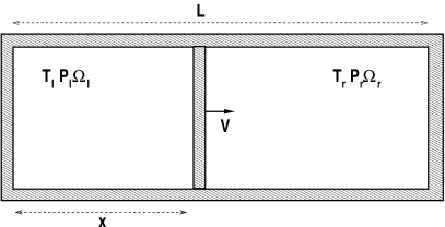
Figure 1: Sketch of the adiabatic piston. The subscripts $l$ and $r$ indicate the left and right compartments, respectively.

At the beginning of last century, the above setup was used as experimental device for measuring the ratio $c_{p}/c_{v}$ of the specific heat of gases Ruchardt , that is linked to the period of the piston oscillations. Renewed interest on the problem has lead to recent experiments exp1 ; exp2 .

Meanwhile, several attempts were made to predict the final equilibrium state by using the laws of thermodynamics only, ending in controversial answers. A naive application of the first two laws of thermodynamics lead to the (wrong) conclusion that the equilibrium conditions is $P_{l}/T_{l}=P_{r}/T_{r}$. A more careful treatment curzon shows that the correct answer is $P_{l}=P_{r}$. However, such a condition says nothing about the final position of the piston and gas temperatures, which remain undetermined. Therefore, equilibrium thermodynamics cannot predict the final state. To shed light on the problem one has to cope with the non-equilibrium process that occurs after the clamp removal.

From a microscopic point of view the adiabatic piston problem for ideal gases (non-interacting particles) can be described in terms of a one dimensional model, where the piston is a heavy particle of mass $M$ much larger that the mass $m$ of the gas molecules, which collide elastically with the piston. As argued by Feynman, the system first converges toward a state of mechanical equilibrium with $P_{r}\approx P_{l}$, consistently with the thermodynamic prediction. Then, the pressure fluctuations, which are asymmetric because $T_{l}\neq T_{r}$, very slowly drive the system toward thermal equilibrium $T_{r}=T_{l}$ feynman . In this way the final position of the piston and the thermodynamic quantities are determined.

More recently, the problem was the subject of renewed attention, mainly stimulated by the talk of Lieb at the Statistical Physics Conference in 1998 lieb , and by the connection of this problem with the physics of mesoscopic systems bustamante ; crosi1 and Brownian motors vandenbroeck1 .

Among the first attempts to understand quantitatively the time evolution of the adiabatic piston we mention Crosignani et al. crosignani who introduced a set of ordinary differential equations for the macroscopic observables. However, this model was only able to account for the position of the piston in the state of mechanical equilibrium and not for the final thermodynamic one.

Remaining in the framework of ideal gases, a systematic investigation in statistical mechanics terms, together with numerical simulations, has been carried on in the last decade by Gruber and coworkers gruber1 ; gruber2 ; gruber3 ; morrisgruber02 ; gruberpache02 ; lesne1 ; morrisgruber03 ; lesne . In these works the problem has been examined in several limits (see Ref. gruberlesne for a review). In particular, in the thermodynamic limit taken by letting the system size $L$ and the piston mass $M$ to go to infinity by holding fixed the ratios $\rho_{0}=N/L$ and $R=mN/M$, it has been shown that the system evolution can be reduced to a set of ordinary differential equations for the macroscopic observables (i.e. the gas left/right temperatures, and the moments of the piston velocity). These equations were obtained by using the Liouville and Boltzmann equations. Within such an approach it is possible to control the deviations from Maxwell-Boltzmann distribution for the gas velocities, observed in the simulations, and a whole hierarchy of equations can be written for all moments of the piston velocity. Remarkably, these equations describe not only the reaching of mechanical equilibrium, which comes from the treatment at zero order in $\frac{m}{M}$ lesne1 , but also the final equilibrium state, which comes from the first order terms in $\frac{m}{M}$ lesne . These analytical results have been shown by the same authors to be in agreement with numerical simulations of the ideal gas piston problem. Though it remains open the problem of a detailed description of the early stage of the dynamics in which the presence of shock waves has an important impact on the dynamics. Some recent attempts in this direction can be found in Ref. Mansour .

When the initial pressures are different, the system phenomenology can be described as follows gruberlesne . In a first stage, the piston oscillates driven by the pressure difference. These oscillations are then damped till the “mechanical equilibrium” state, $P_{r}\simeq P_{l}$ but $T_{r}\neq T_{l}$, is reached. Then, as argued by Feynman, it follows a regime controlled by the asymmetry in the fluctuations felt by the left/right walls. This phase is characterized by a very slow approach to the thermodynamic equilibrium, $P_{r}\simeq P_{l}$ and $T_{r}\simeq T_{l}$, with the piston position fluctuating around the middle of the cylinder. In the oscillatory phase, both experiments exp1 ; exp2 , numerical computations and analytical arguments gruberpache02 ; lesne1 ; morrisgruber03 have shown the existence of two different regimes: weak and strong damping, the relevant parameter being $R$. For $R<R_{c}$ the adiabatic oscillations of the piston are weakly damped, while for $R>R_{c}$ they are over-damped, $R_{c}$ being $\mathcal{O}(1)$ lesne1 .

Still in the context of ideal gases, it is worth mentioning some recent approaches based on dynamical systems theory that have been developed by Chernov, Lebowitz and Sinai sinai . In this context, also the case of gases starting from non-equilibrium conditions has been considered lebo1 ; Caglioti . Clearly, the ultimate goal would be to quantitatively understand the behavior of the system for an interacting gas, but this seems to be still too ambitious. Indeed only very few studies analyzed the case of gas composed by interacting particles vanderbroek2 .

In this paper, we consider a limiting case which has the advantage of being more tractable while displaying most of the non-trivial features of the problem. The basic idea of our approach is to assume that the gases in the two compartments are composed of interacting molecules and thus characterized by a relaxation time toward the equilibrium state. Our main hypothesis is that this time is very short compared with all the other characteristic times of the system. In particular, we require that any fluctuation away from equilibrium (which is characterized by homogeneously distributed gas molecules with a Maxwell-Boltzmann velocity statistics) induced by the collision with the piston is re-adsorbed before the new collision with the piston walls. Physically speaking, the efficient re-adsorption of the fluctuations means that the (mechanical) work done by the piston is immediately converted into heat; an obvious consequence is that shock waves are ruled out. For the sake of simplicity, we also assume that the gases follow the perfect gas law. These hypothesis make the problem tractable while retaining the basic phenomenology of the original problem.

Although a microscopic model of a gas able to fulfill the above requirements may sound rather artificial, at a practical level such a “microscopic model” can be easily implemented on a computer. The basic idea is to start with an equilibrium configuration with temperatures $T_{l,r}$ for the gases, and then reinitialize the gas molecules as soon as one particle collides with the piston. The temperatures are recomputed after the collision and used for extracting a new configuration of the gas molecules. The procedure is then repeated. In the following we shall call such a model randomized gas. Even though, no actual interaction among the particles is actually considered, one can think that the re-generation of the gas configuration from an equilibrium one (but with the new temperature) is the result of such “unresolved” interactions.

With the above assumptions for the gas, we will derive a set of ordinary differential equations for the time evolution of the macroscopic quantities describing the state of the system. Indeed the fact that the gas is always homogeneous and following the Maxwell-Boltzmann distribution allows us to compute the joint probability density function that, in a given state of the system, the first colliding gas particle hits the piston in a time $t$ and with a velocity $v$. Then, by averaging over this joint distribution the energy and momentum exchange due to the collisions with the piston, we derive the evolution of the macroscopic observables. The minimal set of variables required to have a closed set of equations is made up of the gas temperatures, the mean piston position, the first and second moment of the piston velocity. The second moment is required for accounting the piston fluctuations which, as argued by Feynman, are crucial for recovering the correct thermodynamic equilibrium feynman ; gruber3 ; lesne . The equations are derived perturbatively up to the first order in $\frac{m}{M}$. As we will see, though with a different approach and assumption, these equations are very similar to those derived by Gruber and coworkers lesne ; lesne1 , in particular at the zeroth order in $\frac{m}{M}$ they are identical.

We compare then the evolution of the system obtained by simulations of the ideal and randomized gas. In particular, the agreement in the first (mechanical) regime is quantitatively perfect in the case of the randomized gas. While in the second regime, which is dominated by the fluctuations, the agreement seems to be only qualitative. Somehow surprisingly, we found that, in this regime, a better quantitative agreement seems to be possible disregarding some $\mathcal{O}(\frac{m}{M})$ terms. However, with such terms excluded the equipartition of energy at equilibrium is violated by the piston. Some hints to explain these findings could come by higher orders terms in the expansion. Unfortunately, the computation of the higher order terms is very cumbersome. Since the newest aspects of our work is in the proposed derivation and in the introduction of the randomized gas model, we present in this paper the all approach up to first order in $\frac{m}{M}$.

The paper is organized as follows. In Sect. II we present our approach based on the collision statistics and derive the equations for the macroscopic observables. In Sect. III we compare the results of the model with those obtained by simulations. Discussions and conclusions can be found in Section IV. In order to avoid long appendices, the technical material, with the detailed derivation and all the formulas needed to make explicit the equations, is presented as electronic supplementary material  epaps .

II Derivation of the macroscopic equations

The underlying idea of our approach is to derive a set of deterministic dynamical equations for the “macroscopic” variables describing the evolution of the thermodynamic state of the system under the assumption that, at any time, the gases in both chambers are perfect and at equilibrium. In other words the gases are able to instantaneously dissipate the fluctuations induced by the collisions with the piston. Thus a Maxwell-Boltzmann equilibrium state holds always in both compartments but, in general, with different temperatures and volumes.

While the above hypothesis define the macroscopic state of the gas, for the piston the problem is more subtle. We would like to describe its motion on times longer than the single collisions, that is to average its instantaneous position and velocity $(X,V)$ over the collisions so to obtain a deterministic (macroscopic) trajectory defined by the average position $x=\overline{X}$ and velocity $v_{x}=\overline{V}$ The symbol $\overline{[\dots]}$ denotes the average over the collisions. As discussed in the introduction, it is crucial to account also for the fluctuations of the piston velocity. For this reason, the second moment of the piston velocity $\overline{V^{2}}$ is included in the description.

In the thermodynamic limit we will consider, one can argue that the fluctuation of the piston position can be safely ignored. This means that in the following we will consider the piston position as a deterministic quantity and we shall use only the mean piston position $x$.

Given the piston position, the gas is characterized by the temperature $T_{l,r}$, and volume $\Omega_{l,r}$, with $\Omega_{l}=x$ and $\Omega_{r}=L-x$ (we assume a 1d geometry for the sake of simplicity). Being perfect gases, the pressures are given by the equation of state $P_{l,r}\Omega_{l,r}=NT_{l,r}$.

In the sequel we show how to derive a set of differential equations for the evolution of $x$, $v_{x}$, $\overline{V^{2}}$ and $T_{l,r}$. In order to keep the presentation as simple as possible, here we shall sketch how the equations can be derived and the averages performed skipping all the algebra of the computation, which is detailed in epaps .

II.1 Macroscopic equations from the collision rule

For the formal derivation of the deterministic equations, we only need the above discussed assumptions and a microscopic ingredient: the elastic collision rules

$$V^{\prime}=V+\frac{2m}{M+m}(v-V)$$

$$v^{\prime}=v-\frac{2M}{M+m}(v-V)\,.$$ (1)

Primes denote postcollisional velocities, and $v$ the colliding gas particle velocity. The quantities we are interested in are the time derivatives of the macroscopic observables

$$\frac{{\rm d}x}{{\rm d}t}=v_{x}$$ (2)

$$\frac{{\rm d}v_{x}}{{\rm d}t}=\left\langle V^{\prime}-V\right\rangle$$ (3)

$$\frac{{\rm d}\overline{V^{2}}}{{\rm d}t}=\left\langle V^{\prime 2}-V^{2}\right\rangle$$ (4)

$$\frac{{\rm d}T_{l,r}}{{\rm d}t}=m\left\langle v^{\prime 2}-v^{2}\right\rangle_{l,r}\,,$$ (5)

where we set the Boltzmann constant $k_{B}=1$. The time derivatives should be computed starting from the collision rules as the averages $\langle[\dots]\rangle_{l,r}=\overline{[\dots]}_{l,r}/\overline{\delta t}$ suggest, $\overline{\delta t}$ being the mean collisions time (for a more precise and operative definition see Sect II.3). The subscripts ${l,r}$ denote averages performed over the collisions with particles residing on the left/right compartments.

It is useful to introduce $\sigma^{2}_{V}=\overline{V^{2}}-\overline{V}^{2}$ which evolves as

$$\frac{{\rm d}\sigma^{2}_{V}}{{\rm d}t}=\left\langle V^{\prime 2}-V^{2}\right\rangle-2v_{x}\frac{{\rm d}v_{x}}{{\rm d}t}\,,$$ (6)

where we used Eqs. (3) and (4). It should be noted that, at this level, the piston is completely described by $v_{x}$ and $\sigma_{V}^{2}$. This amounts to assume that its velocity distribution is Gaussian

$$P(V)=\frac{1}{\sqrt{2\pi\sigma^{2}_{V}}}e^{-\frac{(V-v_{x})^{2}}{2\sigma^{2}_{V}}}\,.$$ (7)

Since at the initial time $t=0$, one starts with $v_{x}=0$ and $\sigma_{V}^{2}=0$, the above probability distribution is initially a $\delta$ function. Plugging (II.1) into (3-5), we obtain

$$\frac{{\rm d}v_{x}}{{\rm d}t} = N\frac{2m}{M\!+\!m}(\langle v\rangle\!-\!\langle V\rangle)$$ (8)

$$\frac{{\rm d}\sigma^{2}_{V}}{{\rm d}t} = N\frac{4m}{(m\!+\!M)^{2}}\left[\!-\!M\langle\sigma^{2}_{V}\rangle\!+\!m\langle v^{2}\rangle\!+\!(M\!-\!m)\langle vV\rangle\!\right.$$ (9)

$$- \left.(m\!+\!M)v_{x}\langle v\rangle\!+\!(m\!+\!M)v_{x}\langle V\rangle\!-\!M\langle v_{x}^{2}\rangle\right]$$

$$\frac{{\rm d}T_{l}}{{\rm d}t} = \frac{4Mm}{(M\!+\!m)^{2}}\left[M\langle\sigma_{V}^{2}\rangle_{l}+M\langle v_{x}^{2}\rangle_{l}\right.$$ (10)

$$- \left.(M\!-\!m)\langle Vv\rangle_{l}-m\langle v^{2}\rangle_{l}\right]\,,$$

$$\frac{{\rm d}T_{r}}{{\rm d}t} = \frac{4Mm}{(M\!+\!m)^{2}}\left[M\langle\sigma_{V}^{2}\rangle_{r}+M\langle v_{x}^{2}\rangle_{r}\right.$$ (11)

$$- \left.(M\!-\!m)\langle Vv\rangle_{r}-m\langle v^{2}\rangle_{r}\right]\,.$$

The equation for $\sigma^{2}_{V}$ (9) is obtained from (6) and (4) by using the collision rules (II.1). In (8) and (9), the prefactor $N$ appears as a result of a time rescaling, that sets the time unit to the average collision time, which is order $1/N$. Said differently, the change of the gas temperatures due to the collision with the piston is order $1/N$.

Notice that, for reasons that will become clear in the following, the average of the type $\langle V\,v\rangle$ is different from $v_{x}\langle v\rangle$. We anticipate that this difference is not due to a breakdown of molecular chaos hypothesis (as one may naively think) but to the fact that the collision statistics depends on the instantaneous value of the piston velocity. More explicitly, $v_{x}\langle v\rangle$ represents only the zeroth order term of $\langle V\,v\rangle$, and a term coming from the fact that $V$ is a fluctuating quantity will also appear.

Notice also that the above equations conserve the total (gas plus piston) energy

$$E=\frac{RM}{m}\frac{T_{l}+T_{r}}{2}+\frac{M}{2}(v_{x}^{2}+\sigma^{2}_{V})\,.$$ (12)

The consistent (first order in $\frac{m}{M}$) equations can then be obtained from (8-11) by expanding the various prefactors, performing the limit $N\to\infty$ and suitably expanding around it. Since the procedure is delicate, we proceed step by step.

II.2 Thermodynamic limit and formal expansion of the equations

First of all we have to specify the limiting procedure, that as explained in gruberlesne can be done in different ways. We are interested in the limit $N,M,L\to\infty$ in which we keep fixed $\rho_{0}={N}/{L}$ and the nondimensional mass ratio $R={Nm}/{M}$. We have now to expand around this limit retaining all terms which are first order in $\frac{m}{M}$ (and consequently at the first order in $1/N$). Aiming to make explicit the zeroth and first order terms we formally write the averages as:

$$\langle[\dots]\rangle=\langle[\dots]\rangle^{(0)}+\langle[\dots]\rangle^{(1)}\,,$$ (13)

where the first and second terms on the r.h.s are the zeroth and first order terms of the expansion. How to explicitly perform such an expansion will be explained in the following subsections. We warn the reader that for maintaining the notation as compact and explicit as possible in the following we adopt the convection to indicate with $\langle[\dots]\rangle^{(1)}$ all averages which are $\mathcal{O}(\frac{m}{M})$ irregardless if this comes from the expansion of the average or from the averaged quantity. For instance, by direct inspection of Eq. (9) at equilibrium, one easily realizes that $\sigma^{2}_{V}$ is $\mathcal{O}(\frac{m}{M})$. Therefore, we shall always indicate its average with $\langle\sigma^{2}_{V}\rangle^{(1)}$. Finally, notice also that all the terms involving powers of $(V-v_{x})$ vanish at the zeroth order. Keeping in mind these simplifications, the (expanded) equations become:

$${}\frac{{\rm d}v_{x}}{{\rm d}t}\!\! = \!\!2R\langle v-v_{x}\rangle^{(0)}+2R\left[\langle v-v_{x}\rangle^{(1)}-\langle V-v_{x}\rangle^{(1)}-\frac{m}{M}\langle v-v_{x}\rangle^{(0)}\right]$$ (14)

$${}\frac{{\rm d}\sigma^{2}_{V}}{{\rm d}t}\!\! = \!\!4R\left[-\langle\sigma^{2}_{V}\rangle^{(1)}+\frac{m}{M}\langle(v-v_{x})^{2}\rangle^{(0)}+\langle(V-v_{x})v\rangle^{(1)}+\langle(V-v_{x})v_{x}\rangle^{(1)}\right]$$ (15)

$${}\frac{{\rm d}T_{l}}{{\rm d}t}\!\! = \!\!4m\!\left\{\!\langle v_{x}(v_{x}\!-\!v)\rangle_{l}^{(0)}\!+\!\left[\!\langle v_{x}(v_{x}\!-\!v)\rangle_{l}^{(1)}\!\!\!-\!2\frac{m}{M}\langle v_{x}^{2}\rangle_{l}^{(0)}\!\!+\!3\frac{m}{M}\langle v_{x}v\rangle^{(0)}_{l}\!\!+\!\langle\sigma_{V}^{2}\rangle^{(1)}_{l}\right.\right.-\left.\left.\langle(V\!-\!v_{x})v\rangle^{(1)}_{l}\!\!-\!\frac{m}{M}\langle v^{2}\rangle^{(0)}_{l}\!\right]\!\right\}$$ (16)

$${}\frac{{\rm d}T_{r}}{{\rm d}t}\!\! = \!\!4m\!\left\{\!\langle v_{x}(v_{x}\!-\!v)\rangle_{r}^{(0)}\!+\!\left[\!\langle v_{x}(v_{x}\!-\!v)\rangle_{r}^{(1)}\!\!\!-\!2\frac{m}{M}\langle v_{x}^{2}\rangle_{r}^{(0)}\!+\!3\frac{m}{M}\langle v_{x}v\rangle^{(0)}_{r}\!\!+\!\langle\sigma_{V}^{2}\rangle^{(1)}_{r}\right.\right.-\left.\left.\langle(V\!-\!v_{x})v\rangle^{(1)}_{r}\!\!-\!\frac{m}{M}\langle v^{2}\rangle^{(0)}_{r}\!\right]\!\right\}\,.$$ (17)

Before sketching the way the above averages can be computed (see Sect. II.3 and epaps ) we briefly discuss some properties of the above equations.

The first observation is that Eqs. (14-17) ensure the energy conservation (12) both at the zeroth and first order, meaning that the expansion is consistent. Notice also that the relative importance of the various terms is not the same at all times. As the system evolves, their relative weights change corresponding to the different stages of the evolution, briefly summarized in the introduction and detailed in the following. For example, consider $\sigma^{2}_{V}$. At the beginning $\sigma^{2}_{V}=0$, then it grows until it reaches its equilibrium value. Consequently, the terms which involve the velocity fluctuations are not important at the beginning. While they become $\mathcal{O}(\frac{m}{M})$ and play a crucial role in the final stage of the system evolution. The opposite is true for the terms involving the average drift $v_{x}$, which is close to zero in the second (Brownian) stage of the evolution, and large in the first (mechanical) part of the system evolution. Among the terms involving the piston velocity fluctuations, we should mention a special role played by those in which it does not (explicitly) appear $\sigma^{2}_{V}$. These are the terms of the form $\langle(V-v_{x})v_{x}\rangle^{(1)}_{l,r}$ and $\langle(V-v_{x})v\rangle^{(1)}_{l,r}$, as we will see they will be both proportional to $\sigma^{2}_{V}$ and, as anticipated, find their origin in the way the fluctuations of $V$ affect the collision statistics (see next subsections and the supplementary material epaps ). However, a closer inspection shows that $\langle(V-v_{x})v_{x}\rangle^{(1)}_{l,r}$ is very small at all times. In the first stage the fluctuations are negligible while in the second stage the average drift is very small. Though we retained this term in the equations and in the numerical simulations, one can show that they can be removed without problem. Differently the terms $\langle(V-v_{x})v\rangle^{(1)}_{l,r}$ are very important in the final stage of the evolution and, as discussed below, for obtaining the correct equilibrium state.

We are still left with performing the infinite volume limit. We anticipate here that all the terms appearing in the averages are proportional to either $1/x$, when coming from a left-chamber average, or $1/(L-x)$ when coming from a right-chamber average. There is no other dependence on $x$ or $L$ in equations (2-5) and, consequently, Eqs. (14-17). This implies that one can simply introduce the hydrodynamic time $t_{H}=t/L$ and the rescaled $x$ coordinate $x_{H}=x/L$. With this rescaling, $L$ does not appear anymore in the equations and there is no need to perform the limit, meaning that there are no corrections to the results due to finite size effects. For a simpler comparison with the simulations, we will keep writing in the following the equations for finite values of $L$; the corresponding expressions in the hydrodynamic time can be simply obtained with the above substitution, that in practice corresponds to set $L=1$.

II.2.1 Equation at the $0^{th}$ order in $\frac{m}{M}$: Mechanical Regime

Let us start a closer inspection of the equations starting from the zeroth order terms, i.e. assuming $\frac{m}{M}\to 0$. The velocity fluctuations of the piston are ignored (meaning the motion of the piston is purely deterministic) and the final equilibrium position depends on the initial conditions. The result is anyway nontrivial. As discussed in crosignani ; lesne1 , having considered the dynamics and not only the thermostatics (which only tells us the equality of pressures), we can now determine the mechanical equilibrium position. In the sequel, we shall show that at the zeroth order in $\frac{m}{M}$ we obtain, by using a different approach, the same equations of Gruber and coworkers lesne1 , and following them we sketch how the mechanical equilibrium point can be computed.

For obtaining the equations at the $0^{th}$ order, we need to set $\frac{m}{M}=0$ and to ignore all averages indicated with the superscript ⁽¹⁾ in (14), (16) and (17). In other words we only need the averages

$$\langle v\rangle_{l}^{(0)} = \ \frac{T_{l}}{2xm}\left[1-\mathrm{erf}\left(v_{x}\sqrt{\frac{m}{2T_{l}}}\,\right)\right]$$ (18)

$$\langle v\rangle_{r}^{(0)} = -\frac{T_{r}}{2(L-x)m}\left[1+\mathrm{erf}\left(v_{x}\sqrt{\frac{m}{2T_{r}}}\,\right)\right]\,,$$

with $\mathrm{erf}(x)=2/\sqrt{\pi}\int_{0}^{x}\mathrm{d}z\exp(-z^{2})$, and the averages

$$\langle v_{x}\rangle^{(0)}_{l}\!\!\!\! = \!\!\frac{v_{x}}{x}\!\!\left[\!\sqrt{\frac{T_{l}}{2\pi m}}e^{-\frac{mv_{x}^{2}}{2T_{l}}}\!-\!\frac{v_{x}}{2}\!+\!\frac{v_{x}}{2}\mathrm{erf}\!\left(v_{x}\sqrt{\frac{m}{2T_{l}}}\,\right)\!\right]$$ (19)

$$\langle v_{x}\rangle^{(0)}_{r}\!\!\!\! = \!\!\frac{v_{x}}{L\!-\!x}\!\!\left[\sqrt{\frac{T_{r}}{2\pi m}}e^{-\frac{mv_{x}^{2}}{2T_{r}}}\!+\!\frac{v_{x}}{2}\!+\!\frac{v_{x}}{2}\mathrm{erf}\!\left(v_{x}\sqrt{\frac{m}{2T_{r}}}\,\right)\!\right]\,.$$

See the supplements epaps for the derivation of the above expressions. Assuming $v_{x}\ll\sqrt{T_{l,r}/m}$ (which is reasonable for realistic values of the physical parameters), and expanding (18) and (19) in $v_{x}$, the equations (14) and (16-17) reads

$$\frac{{\rm d}v_{x}}{{\rm d}t} = \frac{R}{m}\left(\frac{T_{l}}{x}-\frac{T_{r}}{L-x}\right)-\frac{R}{m}\gamma(v_{x},T_{l},T_{r})v_{x}$$ (20)

$$\frac{{\rm d}T_{l}}{{\rm d}t} = -\frac{2T_{l}v_{x}}{x}+2\gamma_{l}(v_{x},T_{l},T_{r})v_{x}^{2}$$ (21)

$$\frac{{\rm d}T_{r}}{{\rm d}t} = \frac{2T_{r}v_{x}}{(L\!-\!x)}+2\gamma_{r}(v_{x},T_{l},T_{r})v_{x}^{2}$$ (22)

where for the friction coefficients it holds $\gamma=\gamma_{l}+\gamma_{r}$ ensuring energy conservation (12) at the $0^{th}$ order; from (18-19), at the lowest order in $v_{x}$ one has:

$$\gamma_{l,r}(v_{x}=0,T_{l},T_{r})=\frac{1}{\Omega_{l,r}}\sqrt{\frac{8mT_{l,r}}{\pi}}\,,$$ (23)

we remind that $\Omega_{l}=x$ and $\Omega_{r}=L-x$. Note that apparently, in the limit $L\to\infty$, $\gamma_{l,r}\to 0$, this is not the case if the hydrodynamic rescaling is properly applied. Indeed, taking the hydrodynamic limit the above expression remains unchanged, keeping in mind that in this case the ”hydrodynamic volumes” are $\Omega^{H}_{l}=x_{H}$ and $\Omega^{H}_{r}=1-x_{H}$. In particular, the damping coefficients go to a finite value also in the hydrodynamic limit. It is worth remarking, that the linearized equations (20-22) coincide with those derived in Ref. lesne1 with a different method. In the absence of friction, one can easily see that they describe a purely adiabatic transformation of a one-dimensional perfect (mono-atomic) gas. Indeed the first term on the r.h.s. of Eqs. (20) is simply the pressure difference on the two sides of the piston, while the first term of Eq. (21) and (22) can be obtained by differentiating with respect to time the equation of an iso-entropic process, namely

$$T_{l}x^{c_{p}/c_{v}-1} = C_{l}$$

$$T_{r}(L-x)^{c_{p}/c_{v}-1} = C_{r}\,,$$ (24)

where $c_{p}/c_{v}=3$ is the specific heats ratio and the initial conditions fix $C_{l,r}=T_{l,r}(0)\Omega_{l,r}^{c_{p}/c_{v}-1}(0)$. In the absence of the friction terms this would give rise to periodic oscillations of the piston. As discussed in crosignani ; lesne1 , the friction terms are responsible for the irreversible evolution toward a state of mechanical equilibrium for which

$$\frac{N\tilde{T}_{l}}{\tilde{x}}=P_{l}=\tilde{P}=P_{r}=\frac{N\tilde{T}_{r}}{L-\tilde{x}}\,$$ (25)

where the tilde indicates the mechanical equilibrium quantities. Notice that in this framework irreversibility naturally emerges as a result of the averaging over the collisions HOO . Eq. (25) is also the result of thermostatics, but it is not enough to determine $\tilde{x}$ and $\tilde{T}_{l,r}$. Indeed, the full dynamics given by (20-22) is needed to predict such mechanical equilibrium point, as shown in the sequel where we briefly summarize the results first derived in Gruber et al. lesne1 . First, notice that (25) together with (12) tell us that $\tilde{T}_{l,f}=2T_{0}\Omega_{l,r}/L$, with $T_{0}=E/N=(T_{l}(0)+T_{r}(0))/2$. So that the equilibrium pressure is $\tilde{P}=2NT_{0}/L$. Second, defining $Z=\sqrt{T_{l}}x-\sqrt{T_{r}}(L-x)$ and by using (20-22) one can easily see that ${\rm d}Z/{\rm d}t=\mathcal{O}(v_{x}^{3})$, which if $v_{x}\ll 1$ means that $Z$ is conserved. $Z=const$ provides the missing condition to determine the mechanical equilibrium. The resulting equation for the equilibrium point is therefore lesne1 :

$$\sqrt{\tilde{T}_{l}}\tilde{x}-\sqrt{\tilde{T}_{r}}(L-\tilde{x})=\sqrt{T_{l}(0)}x(0)-\sqrt{T_{r}(0)}(L-x(0))\,,$$ (26)

which should be solved for $\tilde{x}$ after plugging $\tilde{T}_{l}=2T_{0}\tilde{x}/L$ and $\tilde{T}_{r}=2T_{0}(1-\tilde{x}/L)$.

II.2.2 Equation at the $1^{th}$ order in $\frac{m}{M}$: Brownian Regime

When the first order (in $\frac{m}{M}$) terms are retained, the terms in $\sigma_{V}^{2}$ (among which, as discussed above, we have also to consider the terms $\langle(V-v_{x})v\rangle^{(1)}$ and $\langle(V-v_{x})v_{x}\rangle^{(1)}$) allows for energy exchange among the two compartments mediated by the fluctuation of the piston. Of course, such terms start to play a role once the mechanical regime (described by the $0^{th}$ order terms) is finished, i.e. when the fluctuations of the piston become relevant. This regime driven by the fluctuations results from the expansions in $\frac{m}{M}$ and $1/N$ which, as it happens commonly in Brownian motor-like systems vandenbroeck1 , are intertwined and add new (sometimes unexpected) features to the dynamics. In particular, in this case one can show that Eq. (14-17) evolve toward a nontrivial stable fixed point corresponding to the thermodynamic equilibrium, i.e.:

$$\frac{x_{eq}}{L}=\frac{1}{2}\,,\quad v_{x}=0\,,\quad T_{l}=T_{r}=T_{eq}\,,\quad{\sigma^{2}_{V}}_{eq}=\frac{T_{eq}}{M}\,.$$ (27)

The last equality cannot be explicitly seen from (15), which simply states that at equilibrium $\langle\sigma^{2}_{V}\rangle^{(1)}=\frac{m}{M}\langle v^{2}\rangle^{(0)}+\langle(V-v_{x})v\rangle^{(1)}$. As we discussed, $\langle(V-v_{x})v\rangle^{(1)}\propto\sigma^{2}_{V}$ and with the explicit computation at equilibrium epaps one can see that ${\sigma^{2}_{V}}_{eq}=T_{eq}/M$, which is a pleasant result since it is in agreement with the condition of equipartition of energy. Notice that Eq. (27) suggests to interpret $M\sigma^{2}_{V}=T_{p}$ as the temperature of the piston.

We conclude this subsection mentioning that the above equations are similar with the ones obtained by Gruber, Pache and Lesne lesne . Due to the very long expressions involved in the equations at the first order, we could not decipher whether they are exactly equal. At the end of next section we shall discuss the possible source of differences. However, we stress that in these two works a different approach and different assumptions were made on the gases. In particular, Gruber, Pache and Lesne derived the equations from an expansion of the Boltzmann and Liouvulle equations. In some sense, our and their different assumptions can be seen as two different ways to close the hierarchy of equations to the second order and one should expect the phenomenology of the two equations to be, at least, qualitatively similar.

Section III is devoted to compare the evolution of the macroscopic observables obtained by integrating (14-17) with that of the microscopic model. In the following subsection we detail the procedure by which the averages can be computed.

II.3 Explicitation of the averages

In order to finalize our program we have now to make explicit the averages in (14-17). Let us start by making explicit the formal expression of averages such as $\langle[\dots]\rangle_{l,r}$, which should be interpreted as follows. Denote with $G_{l,r}(t,v|V)$ the probability of having a left/right collision in a time $t$ with a velocity $v$ for the r/l-particle conditioned to a realization in which the piston has velocity $V$, and indicate with $G$ their sum, i.e. $G=G_{l}+G_{r}$, which is normalized to 1. Then performing the average $\langle A(v,V,t)\rangle_{l,r}$ of a generic function $A(v,V,t)$ means:

$$\langle A(v,V,t)\rangle_{l,r}=\frac{\int\mathrm{d}t\int\!\!\!\int\mathrm{d}v\mathrm{d}VP(V)G_{l,r}(t,v|V)\,A(v,V,t)}{\int\mathrm{d}t\int\!\!\!\int\mathrm{d}v\mathrm{d}V\,t\,P(V)G(t,v|V)}\,,$$ (28)

where $\overline{\delta t}=\int\mathrm{d}t\int\!\!\!\int\mathrm{d}v\mathrm{d}V\,t\,P(V)G(t,v|V)$ is the mean collision time.

II.3.1 Derivation of $G_{l,r}(t,v|V)$

Let us now derive $G_{l}$ and $G_{r}$. In particular, we shall compute them in the thermodynamic limit by explicitly considering the terms order $1/N$ and consequently $\frac{m}{M}$. These terms are those entering the averages we indicated with $\langle[\dots]\rangle^{(1)}_{l,r}$.

We start by the equilibrium distribution of the gases, which is uniform in the particle positions $y$ and Maxwell-Boltzmann for the velocities $v$:

$$p_{l}(y,v) = p_{l}(y)p_{l}(v)=\frac{1}{x}\frac{1}{\sqrt{2\pi m^{-1}T_{l}}}e^{-\frac{mv^{2}}{2T_{l}}}$$ (29)

$$p_{r}(y,v) = p_{r}(y)p_{r}(v)=\frac{1}{(L-x)}\frac{1}{\sqrt{2\pi m^{-1}T_{r}}}e^{-\frac{mv^{2}}{2T_{r}}}\,,$$

that, under our assumptions, describe the gases at all times. Note that the above distributions depend (parametrically) on the dynamical variables $x$ and $T_{l,r}$.

From the equilibrium joint distributions (29) we can derive the probability density $g_{l,r}(t|v,V)$ that a particle on the left/right collides in a time $t$ given its velocity $v$ and the macroscopic state of the system defined by the temperatures, the piston position $x$ and velocity $V$ and the equation of state. Of course, most of the weight to such an hitting probability comes from particles that are close to the piston and that have a large (negative) relative velocity with it. These particles are far from the bulk of the gas and in this derivation we assume that we can use the evolution of free particles to compute their hitting time with the piston. Within such an assumption, it is easy to realize that the probability $g_{l,r}(y,v)$ is simply obtained through a change of variables from (29)

$$g_{l}(t|v,V)\! = \!\Theta(t)\Theta\left(\frac{x}{v\!-\!V}\!-\!t\right)\Theta(v\!-\!V)\frac{v-V}{x}$$

$$\approx \Theta(t)\Theta(v\!-\!V)\frac{v-V}{x}$$

$$g_{r}(t|v,V)\! = \!\Theta(t)\Theta\left(\frac{L\!-\!x}{V\!-\!v}\!-\!t\right)\Theta(V\!-\!v)\frac{V\!-\!v}{L\!-\!x}$$

$$\approx \!\Theta(t)\Theta(V\!-\!v)\frac{V\!-\!v}{L\!-\!x}\,,$$

$\Theta$ being the unitary step function. Note that in the second expression we ignored the second $\Theta$ function. This is justified by the fact that $t$ indicates the time between two consecutive collisions, which for $N\gg 1$ is always much shorter than the time needed for a particle to travel along a whole chamber. Further, considering only positive times, the functions $g_{l,r}(t,v|V)$ do not depend on $t$. We shall then use the compact notation $f_{l,r}(v|V)=g_{l,r}(t,v|V)$. Notice also that we use the instantaneous piston velocity $V$ and not its average $v_{x}$, while we ignore the fluctuations in position. Moreover, we neglected possible correlations between the velocities and positions, which amounts to implicitly assume molecular chaos.

Given $g_{l,r}(t|v,V)$, the joint probability of having an impact of a particle with $v$ in a time $t$ is :

$$g_{l,r}(t,v|V)=g_{l,r}(t|v,V)p_{l,r}(v)\,.$$ (32)

The probabilities $F_{l,r}(t_{m})$ that a left/right particle collides in a time $\leq t_{m}$ is then given by

$$F_{l,r}(t_{m})\!=\!\!\int_{0}^{t_{m}}\!\!\!\!\!\mathrm{d}t\!\!\int_{-\infty}^{\infty}\!\!\!\!\!\mathrm{d}v\ g_{l,r}(t,v|V)\!=\!t_{m}\!\!\int_{-\infty}^{\infty}\!\!\!\!\!\mathrm{d}vf_{l,r}(v|V)$$ (33)

which we rewrite as

$$F_{l,r}(t_{m})=t_{m}H_{l,r}(x,V,T_{l,r})\,,$$ (34)

with

$$H_{l}(x,V,T_{l})\!=\!\int_{V}^{\infty}\!\!\!\mathrm{d}v\frac{v\!-\!V}{\sqrt{2\pi m^{-1}T_{l}}x}e^{-\frac{mv^{2}}{2T_{l}}}$$ (35)

$$H_{r}(x,V,T_{r})\!=\!\int_{-\infty}^{V}\!\!\!\!\mathrm{d}v\frac{V\!-\!v}{\sqrt{2\pi m^{-1}T_{r}}(L\!-\!x)}e^{-\frac{mv^{2}}{2T_{r}}}\,.$$

In the following we will use the shorthand notation $H_{l,r}=H_{l,r}(x,V,T_{l,r})$ and $h_{l,r}=H_{l,r}(x,v_{x},T_{l,r})$.

Considering that we have $N$ particles on both the left and right, the probability densities that one of them on the left/right impacts the piston in $x$ with a velocity $v$ are given by

$$G_{l}(t_{m},\!v)\!=\!N\left[1\!-\!F_{l}(t_{m})\right]^{N\!-\!1}\!\left[1\!-\!F_{r}(t_{m})\right]^{N}\!f_{l}(v|V)$$

$$G_{r}(t_{m},\!v)\!=\!N\!\left[1\!-\!F_{r}(t_{m})\right]^{N\!-\!1}\!\left[1\!-\!F_{l}(t_{m})\right]^{N}\!f_{r}(v|V).$$ (36)

We can now perform the limit $N\!\to\!\infty$ and $t_{m}\!\to\!0$ holding $Nt_{m}\!=\!\tau$ fixed. Noticing that $F_{l.r}(t_{m})\!\to\!\tau H_{l,r}/N$ and expanding $[1\!-\!F_{l,r}]^{N}\!=\!\exp[N\ln(1\!-\!F_{l,r})]\approx\exp[N(-F_{l,r}-F_{l.r}^{2}/2)]$ and retaining terms only up to $1/N$, we find

$$G_{l,r}(\tau,v|V)\!=\!\left[1\!+\!\frac{H_{l,r}\tau}{N}\!-\!\frac{H^{2}_{l}\!+\!H_{r}^{2}}{2N}\tau^{2}\right]\!\tilde{G}_{l,r}(\tau,v|V)$$ (37)

with

$$\tilde{G}_{l,r}(\tau,v|V)=e^{-\tau(H_{l}+H_{r})}f_{l,r}(v|V)\,.$$ (38)

By recalling that $N=MR/m$, and aiming to retain only the first order $\frac{m}{M}$ terms (37) can be rewritten as

$$G_{l,r}(\tau,v|V)\! = \!\tilde{G}_{l,r}(\tau,v|V)\!+\!$$

$$\frac{m}{M}\left(\frac{h_{l,r}\tau}{R}\!-\!\frac{(h^{2}_{l}\!+\!h_{r}^{2})}{2R}\tau^{2}\right)\tilde{G}_{l,r}(\tau,v|v_{x})$$

where we substituted $h$ in place of $H$ and $v_{x}$ in place of $V$ in the part which is already at the first order in $\frac{m}{M}$. However another contribution to the ${\mathcal{O}}(\frac{m}{M})$ term comes from the expansion of the first term in (II.3.1).

II.3.2 Expansion of the average

We need now to further expand (II.3.1) in $V$ around $v_{x}$, this can be accomplished by Taylor expanding $\tilde{G}$

$$\tilde{G}(\tau,v|V) = \tilde{G}(\tau,v|v_{x})+\partial_{V}\tilde{G}(\tau,v|v_{x})(V-v_{x})$$ (40)

$$+ \frac{1}{2}\partial^{2}_{V}\tilde{G}(\tau,v|v_{x})(V-v_{x})^{2}.$$

Noticing that $\int\mathrm{d}VP(V)(V-v_{x})=0$ and that $\int\mathrm{d}VP(V)(V-v_{x})^{2}=\sigma^{2}_{V}$ we can write, for example, the (expanded) average collision time:

$$\overline{\delta t} = \frac{1}{h_{l}+h_{r}}\left[1-\frac{m}{M}\frac{h_{l}^{2}+h_{r}^{2}}{R(h_{l}+h_{r})^{2}}\right.$$

$$+ \left.\frac{h_{l}+h_{r}}{2}\sigma^{2}_{V}\int\!\!\!\int\mathrm{d}t\,\mathrm{d}v\,t\,\partial^{2}_{V}\tilde{G}(\tau,v|v_{x})\right].$$

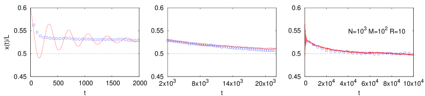
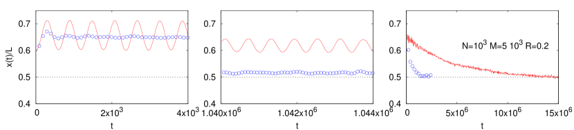
Figure 2: (Color online) (top) Comparison between the evolution of the piston position $x(t)$ in a simulation of an ideal gas (red solid line) and of the randomized model (blue, open circles). In both models we set $N=1000$, $M=100$ and $L=2000$ corresponding to $R=10$, at time zero $T_{l}=40$, $T_{r}=60$ and $x=0.6L$. To have a cleaned curve we performed an average of about $100$ independent realizations. (bottom) The of (top) with $N=1000$, $M=5000$ and $L=2000$ corresponding to $R=0.2$, and the initial state set as $T_{l}=150$, $T_{r}=50$ and $x=0.6L$. Here, for the ideal gas, the oscillations last for a much longer time and are damped very slowly before the Brownian motor like regime sets in; while the randomized gas is much more efficient in damping the oscillations.

Finally, we can write the correct expansion of (28) at the first order in $\frac{m}{M}$, by plugging all the expanded terms in (28) to have the zero and first order terms of the average of a generic observable, $\langle A\rangle_{r,l}=\langle A\rangle^{(0)}_{r,l}+\langle A\rangle^{(1)}_{r,l}$. The result is:

$${}\langle A\rangle^{(0)}_{r,l}=\!(h_{l}\!+\!h_{r})\int\!\!\!\!\int\!\!\!\!\int\!\mathrm{d}\tau\mathrm{d}v\mathrm{d}V\,P(V)\,\tilde{G}_{l,r}(\tau,\!v|v_{x})\,A$$ (43)

$${}\langle A\rangle^{(1)}_{r,l}=\!\int\!\!\!\!\int\!\!\!\!\int\!\mathrm{d}\tau\mathrm{d}v\mathrm{d}V\,P(V)\bigg{[}\partial_{V}\tilde{G}_{l,r}(\tau,\!v|v_{x})(V\!-\!v_{x})$$

$${}+\!\frac{1}{2}\partial^{2}_{V}\tilde{G}_{l,r}(\tau,\!v|v_{x})(V\!-\!v_{x})^{2}\!\bigg{]}\,A\!+\!\left[\!\frac{m}{M}\frac{h_{l,r}}{R(h_{l}+h_{r})}\!-\!\sigma_{V}^{2}\right.$$

$${}\left.\frac{(h_{l}+h_{r})^{2}}{2}\int\!\!\!\!\int\!\!\mathrm{d}t\,\mathrm{d}v\,t\,\partial^{2}_{V}\tilde{G}(\tau,\!v|v_{x})\right]\int\!\!\!\mathrm{d}v\,f_{l,r}(v|v_{x})A$$

which can be used to compute all the averages in (14-17). However we mention that there are exceptions to the above recipe. For instance, the average of $A=(V-v_{x})^{2}$, whose result is $\langle\sigma^{2}_{v}\rangle^{(1)}$ and not $\langle\sigma^{2}_{v}\rangle^{(0)}$. This is due to the convention adopted for the average: remember that we chose to write the superscript ⁽¹⁾ also when the $\frac{m}{M}$ order comes from the averaged quantity and not from the expansion of the collision distribution, like in this case.

Notice that in the first term of the r.h.s of (43), as for the average collision time, we expanded $\tilde{G}$ with the aid of (40). Depending on the observable $A$, which may have or not a linear term in $V-v_{x}$, also the first derivative of $\tilde{G}$ may appear.

III Comparison between model and molecular dynamics simulations

In this section we compare the evolution of the macroscopic observables given by (14-17) with numerical simulations of the microscopic model. We consider two kinds of microscopic simulations: the ideal and the randomized gas. The latter is meant to fulfill the assumptions we made on the gas in deriving the equations. Let us now better clarify how this is realized.

From a computational point of view, it is very easy to realize the randomized gas, the idea is to let the gases relax in an artificial manner through a randomization procedure. More precisely, the simulations are performed in the following way: we generate an equilibrium configuration of the system, corresponding to given values of the macroscopic observables. Then the system is let to evolve up to the first collision of the piston without interactions among the gas particles. After the collision, the energy of the gas containing the colliding particle changes; the fast relaxation of the system is mimicked by updating the gas temperature (corresponding to the new energy) and redrawing an equilibrium configuration of the gases corresponding to the new temperatures (and volumes). Then the process is iterated. Notice that in this way one keeps track of all the observables except the piston velocity fluctuation, which needs some kind of average to be defined/measured. Collisions are evaluated, as for the ideal gas, with an event driven algorithm.

In Figure 2 we show the evolution of the piston position by numerical simulations of the ideal and randomized gas for two different values of $R$ (namely $R=10$ (top) and $R=0.2$ (bottom). As discussed in the introduction (see gruberlesne ; lesne for a more detailed treatment) these two choices correspond to the case of strongly and weakly damped oscillations, respectively. In both cases one has two regimes: mechanical and Brownian. The former is characterized by damped oscillations of the piston, which in the strongly damped case are very few or nonexistent. For the ideal gas, as discussed by Gruber et al. lesne1 ; lesne ; gruberlesne the detailed damping of the oscillations depends on the presence of shock waves, which are absent in the randomized gas. In fact, the latter is damped much more efficiently than the former. As shown in the bottom panel, for $R=0.2$ the evolution is weakly damped and many oscillations are observable. In this case, the piston is very slow and the gases perform quasi-adiabatic oscillations, which are damped more and more mildly as $R\to 0$. Again, also in this case the damping appear to be much more efficient in the randomized case.

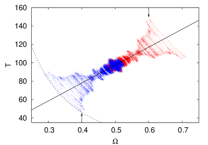
Figure 3: (Color online) Evolution of the system in the temperature volume ($T\Omega$) plane. The dotted line indicates the adiabatic phase $T\propto V^{-2}$, while the solid straight line the isobar that characterizes the final phase (Brownian motor like regime). The rightmost arrow indicates the initial state of the gas in left compartment $T_{l}(0)=150$ $\Omega_{l}(0)=x(0)=0.6L$ which evolves (red dots) toward the final equilibrium in the middle. The leftmost arrow indicate the initial state of the gas in left compartment $T_{l}(0)=150$ $\Omega_{r}(0)=L-x(0)=0.4L$ which evolves (blue dots) toward the final equilibrium in the middle. The simulation is done with the ideal gas, for which the initial oscillations are much more evident that for the randomized one.

The Brownian motor-like regime vandenbroeck1 , occurs when the oscillations are completed damped, i.e. the mechanical equilibrium is realized with approximately equal pressures $P_{l}\approx P_{r}$, which differ only for terms $\mathcal{O}(\frac{m}{M})$. From now on, both the ideal and randomized gas remain in a state of marginal equilibrium approximately along the isobar $T_{l}/x=T_{r}/(L-x)$, which is the prediction of thermodynamics (shown in Fig. 3 for the ideal gas only). The Brownian motor-like mechanism is responsible for heat transfer from the warmer to the colder chamber mediated via the piston fluctuations vandenbroeck1 ; vanderbroek2 . This stage occurs on a long timescale (proportional to $M$). For realistic values of the various parameters, one can realize that the timescales necessary for reaching the thermodynamic equilibrium state are enormous. It is therefore very difficult to observe this regime in experiments, and well controlled numerical simulations are mandatory. In the final state the two chambers have the same temperatures and the piston fluctuates reaching equipartition with the same temperature. It is worth noticing that for the ideal gas, since the molecules interact only through the collisions with the piston, the probability distribution of the velocities of the gas molecules may (and actually do) deviate sensibly from the Maxwell-Boltzmann distribution that is recovered only after the reaching of the final equilibrium state gruberlesne ; lesne . By construction, this problem is not present in the randomized gas which is forced to remain Maxwell-Boltzmann.

In the following we shall compare the evolution of the macroscopic equations with the simulations.

III.1 Mechanical regime

We start the comparison by considering the oscillatory regime in the weakly damped case. Here we know from previous studies lesne1 that the model is able to correctly predict the period of the oscillations.

The period of the oscillations in the model can be estimated from the linearized dynamics at the zeroth order in $\frac{m}{M}$, Eqs. (20-22). As discussed in Sect. II.2, the oscillations will occur around a mechanical equilibrium position $\tilde{x}$ defined by Eq. (26). Then to recover the period of the oscillations it is enough to linearize (20-22) around the mechanical equilibrium state defined by $\tilde{x}$, $\tilde{T}_{l,r}$ and $\tilde{v}_{x}=0$. Linearizing (21-22) one can easily recognize that the equation define an iso-entropic process, i.e. (24), meaning that $T_{l}(x)=\tilde{T}_{l}(\tilde{x}/x)^{c_{p}/c_{v}-1}$ and $T_{r}(x)=\tilde{T}_{r}[(L-\tilde{x})/(L-x)]^{c_{p}/c_{v}-1}$, which plugged in (20) and expanding in $\delta x=x-\tilde{x}$ lead to the equation of a damped oscillator:

$$\frac{{\rm d}^{2}\delta x}{{\rm d}t^{2}}+\frac{R}{m}\gamma\frac{{\rm d}\delta x}{{\rm d}t}+\frac{R}{mN}\frac{c_{p}}{c_{v}}\frac{\tilde{P}L}{\tilde{x}(L-\tilde{x})}\delta x=0\,,$$ (44)

where we recall that $c_{p}/c_{v}=3$ and $\tilde{P}=2NT_{0}/L$ (see Sec. II.2.1). Since the friction coefficient does not modify the period one immediately gets:

$$\mathcal{T}=2\pi\sqrt{\frac{Nm\tilde{x}(L-\tilde{x})}{R(c_{p}/c_{v})\tilde{P}L}}\,,$$ (45)

this formula is at the basis of the measurement of the specific heat ratio in experiments Ruchardt .

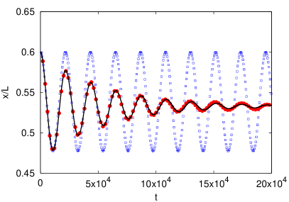
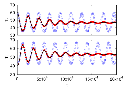
Figure 4: (Color online) Comparison between the simulations of the non-interacting 1D gas, the randomized one and the prediction given by the macroscopic equations. The parameters are: $T_{l}=40$, $T_{r}=60$, $L=12000$, $x_{0}/L=0.6$, $M=10^{5}$, $N=10^{3}$ corresponding to $R=0.01$. (top) Evolution of the piston position. (bottom) Evolution of the temperatures. Blue open squares refer to the ideal gas and red filled circles to the randomized gas, the solid line is the model (14-17).

In Fig. 4, we compare the ideal gas simulations with that of the randomized gas and the numerical integration of the determinist equations (14-17). As one can see, the ideal and randomized gas have the same period, while the damping is different, and the model is in perfect agreement with the randomized gas simulations. Integrating the equation at the zeroth order, we find $\tilde{x}=6.39\times 10^{3}$ which agrees with the predicted value (26) and Eq. (45) predicts $\mathcal{T}=2.17\times 10^{4}$ which is in very good agreement with the the measured period in both the randomized and ideal gas.

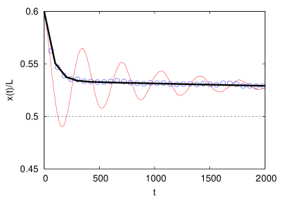
Figure 5: (Color online) The same as the leftmost plot of Fig. 2(top) with superimposed the thick black line superimposing on randomized gas data (blue empty circles) is obtained by the numerical integration of (14-17). The agreement of the model with the randomized gas is perfect also for the temperatures (not shown).

We mention that in Ref. lesne1 a detailed study of the period of the oscillations was reported. Since our linearized equations coincide with those of Ref. lesne1 , we shall not repeat here this study. It is however interesting to compare the first stage of the evolution of the ideal and randomized gas with the model in the case of strong damping. In Fig. 5 we show the leftmost plot of Fig. 2 (top), as one can see although the model is unable to reproduce the oscillation of the ideal gas, its evolution coincides with that of the randomized gas.

As discussed in Ref.gruberlesne , estimating the decay rate of the oscillations for the ideal gas is a nontrivial task, since it requires a detailed study of the dissipation mechanisms of the shock waves created by the piston motion. These shock waves survive for a long time in the ideal gas, while they lifetime is expected to be shorter in the presence of interactions, which should be able to decrease their coherence. The randomized gas represents a sort of limiting case of interaction in which the shock waves are completely absent. Most likely the absence of shock waves is at the origin of the faster damping of the oscillations in the randomized gas and of the very good agreement between its evolution and the one obtained from the macroscopic equations. It would be interesting to investigate the transition between weak and strong damping in the randomized model. This is far from the aim of the present paper, however the above results suggest that the critical value of $R$ for the transition will probably be smaller (but of the same order) of that of the ideal gas which is order unity.

III.2 Brownian motor-like regime

As the mechanical equilibrium is reached $P_{l}\approx P_{r}$, the system slowly evolves, along an approximate isobar, driven by fluctuations toward the thermodynamical equilibrium defined by Eq. (27), which is the (stable) fixed point of the ordinary differential equations (14-17).

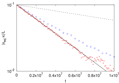
Figure 6: (Color online) Comparison between the molecular dynamics of a non-interacting 1D gas and the model in the Brownian motor-like regime. Simulations have been performed setting the initial state as $T_{l}=40$, $T_{r}=60$ and $x(0)=0.4L$ with $M=500$ and $L=12N$ with $N=10^{4}$: red triangles refer to the randomized gas and the blue squares to the ideal gas, respectively. The dashed line is the prediction of the macroscopic equation, the solid line (which perfectly superimposes on the randomized gas data) is explained in the text. The simulation data are obtained by performing an average over about $10$ realizations to reduce the fluctuations.

We shall now compare the evolution given by the macroscopic equations with that of the ideal and randomized gases in the Brownian regime. To minimize the possible differences between the ideal and randomized gases we performed a simulation which starts in a mechanical equilibrium state having the gas molecules distributed according to the Maxwell-Boltzmann distribution. For the ideal gas, this might be not the typical situation: usually when the system arrives to the mechanical equilibrium from a non-equilibrium state, it may be strongly non-Maxwellian gruberlesne ; lesne . As exemplified in Fig. 6, where we show the deviation from the final equilibrium of the piston position, $|x-x_{eq}|/L$, the relaxation is exponential. The randomized gas relaxes faster than the ideal one, likely because the latter develops slightly non-Maxwellian distribution (we observed that the difference in the relaxation time tends to diminish as the number of particles is increased). Note that the simulation has been performed with $R>1$ because the time scale for reaching the equilibrium is controlled by $M$; with $N=10^{4}$, as here, working with $R<1$ would have implied the necessity to reach too large time scales to study the relaxation.

As shown in the figure, the macroscopic equations (dashed line) predict a relaxation slower than both the randomized and ideal gases. This came out as a surprise for us, because we were encouraged by the very good agreement in the mechanical regime, discussed in the previous section. With the aim of understanding such a difference we examined all the terms appearing in the macroscopic equations and we realized that the mismatch in the relaxation was due to the terms $\langle(V-v_{x})v\rangle_{l,r}^{(1)}$ that, as discussed in Sect. II.2.2, are those which ensures the equipartition of energy at equilibrium, i.e. the fact that $M{\sigma_{V}^{2}}_{eq}=T_{eq}$. In particular, eliminating such terms from (14-17) (note that this is not affecting the conservation of energy), we found a perfect agreement between the macroscopic equations, now modified, and the randomized gas, as shown by the solid line in the figure. Nevertheless, with such a modification the energy equipartition is not verified anymore and at equilibrium $M{\sigma_{V}^{2}}_{eq}=2T_{eq}$.

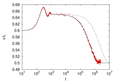
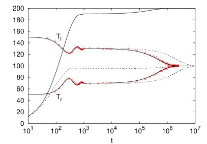
Figure 7: (Color online) (top) Evolution of the piston position for parameter as in Fig. 2(bottom) now plotted in log-lin scale. The (red) symbols refer to the randomized gas simulations, the dashed curve to the evolution predicted by the macroscopic equations and the solid curve (which perfectly superimposes on the simulation data) is explained in the text. (bottom) Same as (top) but for the evolution of the gas temperatures $T_{l}$ and $T_{r}$ as in label. The two curved which start from zero show the evolution of the piston temperature $T_{p}=M\sigma_{V}^{2}$ as obtained from the macroscopic equations (dashed curve which saturates to $T_{p}\approx 100$ and as explained in the text the solid one which saturates ad $T_{p}\approx 200$.

One may think that the agreement is incidental, and so we did a more severe test. In Fig. 7 we show the evolution of the piston position (top) and of the gas temperatures (bottom) with the simulations of the randomized gas previously shown in Fig. 2(bottom). As one can see, the modified (solid lines) and original (dashed lines) macroscopic equations generate, a part from $\sigma^{2}_{V}$, two indistinguishable dynamics for $x$ and $T_{l,r}$ up to times for which the mechanical equilibrium is reached. Actually for such times the dynamics is essentially given by the zeroth order equations (20-22) which are the same for both the original and modified equations: this explain their behavior in the mechanical regime. As one can see the main difference in the dynamics is that retaining the terms $\langle(V-v_{x})v\rangle_{l,r}^{(1)}$ leads the system to stay for a longer time interval in a state of approximate mechanical equilibrium and thus to a slower relaxation to equilibrium. The evolution of the piston temperature $M{\sigma_{V}^{2}}$ shown in Fig. 7 (bottom) clearly show the difference in the two dynamics, and in particular the breaking of equipartition at equilibrium for the modified dynamics.

It should be stressed that the behaviors shown in the above figures is not related to the peculiar parameters choice as it has been verified in other simulations (not shown).

The picture emerging from this comparison is that the model we introduced goes to the correct equilibrium state and respects the basic physics principles as conservation of energy and its equipartition. On the other hand, the relaxation is slower than the one of the microscopic model it should correspond to (i.e. the randomized gas). As shown in the above figures the terms responsible for this slowing down are the ones coming from the fluctuation of the piston velocity in the expansion of the function $G$. At present we dot not have a definite understanding either of this difference in the dynamics of the macroscopic equations and of the randomized gas, or of the very good agreement between the modified equations and the randomized gas. We suspect that the contribution to the relaxation time of these terms might be counterbalanced by the resummation of higher order terms in the $\frac{m}{M}$ expansion. However, carrying the analysis to higher order terms is very demanding due to the proliferation of terms in the expansion, and therefore we shall not discuss it here.

We conclude this section by mentioning that the equations derived by Gruber and coworkers lesne predict a reasonable relaxation time and equipartition at the same time. We remark that going to higher order in their approach requires to include into the description also higher order moments of the piston velocity, namely $\overline{V^{3}},\dots$; while within our approach the description remains at the level of the second order moment because the statistics is constrained to remain Gaussian (Maxwell-Boltzmann) for the gases and the piston. This may be the origin of the difference between our and their derivation. Their equations at the first order might likely correspond to a resummation of higher order terms in our approach, meaning that their closure with the second moment of the velocity is exact while ours remains only approximate.

IV Conclusions

In the framework of kinetic theory, we derived a set of deterministic equations describing the evolution of the macroscopic variables in the adiabatic piston problem. Our basic assumptions are that at each time the gases in the two compartments are perfect, spatially homogeneous, and described by the Maxwell-Boltzmann statistics. Thus, at the level of simulations, a (randomized) gas model has been introduced with aim to have microscopic model respecting such assumptions. We obtained a set of five ordinary differential equations for the variables that describe the macroscopic state of the system, namely the mean position of the piston, the average velocity of the piston, the temperatures of the gases in the two compartments and the second moment of the piston velocity. The equations are derived up to the first order in $\frac{m}{M}$.

At the zeroth order they describe a deterministic piston characterized by a velocity distribution collapsed on the mean, namely $P(V)=\delta(V-v_{x})$. This is enough to solve the problem of finding the final state of mechanical equilibrium and the result coincides with that derived in Ref. lesne1 by using a different approach.

At the first order the fluctuations of the piston velocity, now assumed to be Gaussian, allow for recovering the correct final thermodynamic equilibrium. Although the evolution of the macroscopic observables provided by this set of equations is in good qualitative agreement with simulations of the randomized gas, we found some quantitative discrepancy for the relaxation timescales.

Apart from the performance in comparing with the simulations, we would like to stress the conceptual aspects of the method we developed. It allows for a transparent description of the macroscopic dynamics of a nontrivial non-equilibrium problem, similarly to how the perfect gas law can be derived from the microscopic collisions by using elementary kinetic theory.

- (1) H.B. Callen, Thermodynamics (J. Wiley ans Sons, New York, 1963).
- (2) R.P. Feynman, Lectures in Physics I (Addison-Wisley, New York, 1965).
- (3) C. Gruber and A. Lesne, in Encyclopedia of Mathematical Physics J.P. Francoise, G. Naber, T.S. Tsun (eds.) (Elsevier, 2006).
- (4) E. Rüchardt, Z. Phys. 30, 58 (1929).
- (5) O.L. de Lange and J. Pierrus, Phys. Rev. E 57, 5520 (1998).
- (6) J. Pierrus and O.L. de Lange, Phys. Rev. E 56, 2841 (1997).
- (7) A.E. Curzon, Am. J. Phys. 37, 404 (1969).
- (8) E. Lieb, Physica A 263, 491 (1999).
- (9) C. Bustamante, J. Liphardt and F. Ritort, Phys. Today 58, 43 (2005).
- (10) B. Crosignani and P. Di Porto, Europhys. Lett. 53, 290 (2001).
- (11) C. Van den Broeck, New J. Phys. 7, 10 (2005).
- (12) B. Crosignani, P. Di Porto and M. Segev, Am. J. Phys. 64, 610 (1996).
- (13) C. Gruber, Eur. J. Phys. 20, 259 (1999).
- (14) C. Gruber and J. Piasecki, Physica A 268, 258 (1999).
- (15) C. Gruber and L. Frachebourg, Physica A 272, 392 (1999).
- (16) G.P. Morriss and C. Gruber, J. Stat. Phys. 109, 549 (2002).
- (17) C. Gruber, S. Pache, Physica A 314, 345 (2002).
- (18) C. Gruber, S. Pache and A. Lesne, J. Stat. Phys. 108, 669 (2002).
- (19) C. Gruber, S. Pache and A. Lesne, J. Stat. Phys. 112, 1177 (2003).
- (20) G.P. Morriss and C. Gruber , J. Stat. Phys. 113, 297 (2003).
- (21) M.M. Mansour, C. Van den Broeck, and E. Kestemont, Europhys. Lett. 69, 510 (2005); M.M. Mansour, A.L. Garcia, and F. Baras, Phys. Rev. E 73, 016121 (2006).
- (22) N. Chernov, J. L. Lebowitz, and Ya. Sinai, J. Stat. Phys. 109, 529 (2002).
- (23) N. Chernov and J.L. Lebowitz, J. Stat. Phys. 109, 507 (2002).
- (24) E. Caglioti, N. Chernov and J.L Lebowitz, Nonlinearity 17, 897 (2004).
- (25) E. Kestemont, C. Van den Broeck and M. Malek Mansour, Europhys. Lett. 49, 143 (2000).
- (26) See EPAPS associated to this paper.
- (27) W.G. Hoover, Time reversibility, computer simulations, and chaos, pg. 47 (World Scientific, Singapore, 2001).