Interaction for Solitary Waves with a Phase Difference in a Nonlinear Dirac Model

Abstract

This paper presents a further numerical study of the interaction dynamics for solitary waves in a nonlinear Dirac field with scalar self-interaction by using a fourth order accurate Runge-Kutta discontinuous Galerkin method. Our experiments are conducted on the Dirac solitary waves with a phase difference. Some interesting phenomena are observed: (a) full repulsion in binary and ternary collisions and its dependence on the distance between initial waves; (b) repulsing first, attracting afterwards, and then collapse in binary and ternary collisions of initially resting two-humped waves; (c) one-overlap interaction and two-overlap interaction in ternary collisions of initially resting waves.

,

1 Introduction

Ever since its invention in 1929 the Dirac equation has played a fundamental role in various areas of modern physics and mathematics, and is important for the description of interacting particles and fields. Consider a classical spinorial model with scalar self-interaction, described by the nonlinear Lagrangian $L=\mathrm{i}\overline{\mbox{\boldmath$\psi$}}\gamma^{\mu}\partial_{\mu}\mbox{\boldmath$\psi$}-m\overline{\mbox{\boldmath$\psi$}}\mbox{\boldmath$\psi$}+\lambda(\overline{\mbox{\boldmath$\psi$}}\mbox{\boldmath$\psi$})^{2}$ from which we may derive the nonlinear Dirac equation

$$\mathrm{i}\gamma^{\mu}\partial_{\mu}\mbox{\boldmath$\psi$}-m\mbox{\boldmath$\psi$}+2\lambda(\overline{\mbox{\boldmath$\psi$}}\mbox{\boldmath$\psi$})\mbox{\boldmath$\psi$}=0,$$ (1)

where the $\gamma^{\mu}$ matrices are defined by

$$\gamma^{0}=\left(\begin{matrix}I&0\\ 0&-I\end{matrix}\right),\gamma^{k}=\left(\begin{matrix}0&\sigma^{k}\\ -\sigma^{k}&0\end{matrix}\right),$$

here $\sigma^{k}$ with $k=1,2,3$, denote the Pauli matrices. The nonlinear self-coupling term $(\overline{\mbox{\boldmath$\psi$}}\mbox{\boldmath$\psi$})^{2}$ in the Lagrangian allows the existence of finite energy, localized solitary waves, or extended particle-like solutions, see e.g. [1]. Several authors have committed themselves to analytically investigating the nonlinear Dirac model [2, 3, 4, 5, 6, 7].

Here we only pay our attention to advances in numerical studies of interaction dynamics of the Dirac solitary waves. Up to now, some reliable, higher-order accurate numerical methods have been constructed to solve the nonlinear Dirac equation (1). They include Crank-Nicholson type schemes [8, 9], split-step spectral schemes [10], Legendre rational spectral methods [11], and Runge-Kutta discontinuous Galerkin (RKDG) methods [12], etc. The interaction dynamics for the solitary wave solutions of (1) were numerically simulated in [8] by using a second-order accurate difference scheme. The authors saw there: charge and energy interchange except for some particular initial velocities of the solitary waves; inelastic interaction in binary collisions; and bound state production from binary collisions. Weakly inelastic interaction in ternary collisions is observed in [12]. The interaction dynamics in the binary and ternary collisions of two-humped solitary waves are first investigated in [13].

However, the experiments carried out in the literatures are all limited to the binary and ternary collisions of the in-phase solitary waves of (1). In this Letter we will devote ourselves to further investigating the interaction dynamics in the binary and ternary collisions of the Dirac solitary waves with an initial phase shift by using a fourth-order accurate RKDG method [12] and report some interesting observations. The RKDG methods adopt a discontinuous piecewise polynomial space for the approximate solutions and the test functions, and an explicit, high-order Runge-Kutta time discretization. It has been demonstrated by various experiments that the fourth-order RKDG method is numerically stable without generating numerical oscillation within a very long time interval, has uniformly numerical convergence-rates, and preserve conservation of the energy and charge. We refer the reader to [12] as well as [13] for a detailed description and more numerical demonstrations.

2 Preliminaries

We restrict our attention to the $(1+1)$-dimensional nonlinear Dirac model (1), and use the same notations $\rho_{E}(x,t)$ and $\rho_{Q}(x,t)$ as ones in [12, 13] to denote the energy and charge densities defined by

$$\rho_{E}(x,t)= \mbox{Im}(\psi_{1}^{*}\partial_{x}\psi_{2}+\psi_{2}^{*}\partial_{x}\psi_{1})+m(|\psi_{1}|^{2}-|\psi_{2}|^{2})-\lambda(|\psi_{1}|^{2}-|\psi_{2}|^{2})^{2},$$ (2)

$$\rho_{Q}(x,t)= |\psi_{1}|^{2}+|\psi_{2}|^{2},$$ (3)

where $\psi_{1}$ and $\psi_{2}$ are two components of the spinor $\mbox{\boldmath$\psi$}(x,t)$. A standing wave solution of the Dirac model (1) is given as

$$\mbox{\boldmath$\psi$}^{sw}(x,t)\equiv\left(\begin{array}[]{l}\psi_{1}^{sw}(x,t)\\ \psi_{2}^{sw}(x,t)\end{array}\right)=\left(\begin{array}[]{l}A(x)\\ \mathrm{i}B(x)\end{array}\right)e^{-\mathrm{i}\Lambda t},\ 0<\Lambda\leq m,$$ (8)

with

$$A(x)=\frac{\sqrt{\frac{1}{\lambda}(m^{2}-\Lambda^{2})(m+\Lambda)}\cosh\big{(}x\sqrt{(m^{2}-\Lambda^{2})}\big{)}}{m+\Lambda\cosh\big{(}2x\sqrt{(m^{2}-\Lambda^{2})}\big{)}},$$ (9)

$$B(x)=\frac{\sqrt{\frac{1}{\lambda}(m^{2}-\Lambda^{2})(m-\Lambda)}\sinh\big{(}x\sqrt{(m^{2}-\Lambda^{2})}\big{)}}{m+\Lambda\cosh\big{(}2x\sqrt{(m^{2}-\Lambda^{2})}\big{)}}.$$ (10)

The Dirac model (1) also has a single solitary wave solution placed initially at $x_{0}$ with a velocity $v$:

$$\mbox{\boldmath$\psi$}^{ss}(x-x_{0},t)=\big{(}\psi_{1}^{ss}(x-x_{0},t),\psi_{2}^{ss}(x-x_{0},t)\big{)}^{T},$$ (11)

where

$$\psi_{1}^{ss}(x-x_{0},t)=\sqrt{\frac{\gamma+1}{2}}\psi_{1}^{sw}(\tilde{x},\tilde{t})+\mbox{sign}(v)\sqrt{\frac{\gamma-1}{2}}\psi_{2}^{sw}(\tilde{x},\tilde{t}),$$ (12)

$$\psi_{2}^{ss}(x-x_{0},t)=\sqrt{\frac{\gamma+1}{2}}\psi_{2}^{sw}(\tilde{x},\tilde{t})+\mbox{sign}(v)\sqrt{\frac{\gamma-1}{2}}\psi_{1}^{sw}(\tilde{x},\tilde{t}),$$ (13)

here $\gamma={1}/{\sqrt{1-v^{2}}}$, $\tilde{x}=\gamma(x-x_{0}-vt)$, $\tilde{t}=\gamma(t-v(x-x_{0}))$, $\psi_{1}^{sw}$ and $\psi_{2}^{sw}$ are defined in (8) and $\mbox{sign}(x)$ is the sign function, which returns $1$ if $x>0$, $0$ if $x=0$, and $-1$ if $x<0$. The function $\mbox{\boldmath$\psi$}^{ss}(x-x_{0},t)$ represents a solitary wave travelling from left to right if $v>0$, or travelling from right to left if $v<0$, and the standing wave $\mbox{\boldmath$\psi$}^{sw}(x-x_{0},t)$ is actually a solitary wave at rest placed at $x_{0}$ or identical to $\mbox{\boldmath$\psi$}^{ss}(x-x_{0},t)$ with $v=0$.

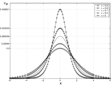
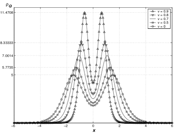
Figure 1: Dependence of $\rho_{Q}$ on $\Lambda$ and $v$. Left: $\Lambda=0.9$; right: $\Lambda=0.1$.

The profile of the solution (8) or (11) is strongly dependent on the parameter $\Lambda$: it is a two-humped solitary wave with two peaks whose locations are determined by $\cosh(2\sqrt{m^{2}-\Lambda^{2}}\tilde{x})=\frac{m^{2}-\Lambda^{2}}{m\Lambda}$ if $0<\Lambda<\frac{m}{2}$; it becomes a one-humped solitary wave with one peak located at $\tilde{x}=0$ if $\frac{m}{2}\leq\Lambda<m$; and $\mbox{\boldmath$\psi$}^{ss}(x-x_{0},t)\equiv 0$ if $\Lambda=m$. Moreover, amplitude of the solitary waves also depends strongly on the velocity $v$: $\rho_{Q}^{ss}(x-x_{0},t)=\gamma\rho_{Q}^{sw}(\tilde{x},\tilde{t})$. Fig. 1 shows that dependence, which will gives different interaction dynamics. It is worth noting that $e^{\mathrm{i}\theta}\mbox{\boldmath$\psi$}^{ss}(x-x_{0},t)$ is still a solitary wave solution of the Dirac model (1), if $\theta$ is a constant.

In the following, our computations will work in dimensionless units, or equivalently, take $m=1$ and $\lambda=\frac{1}{2}$, and adopt the non-reflecting boundary conditions at two boundaries of the computational domain. The domain is covered by some identical cells with area of $0.05$. The numerical algorithm is the $P^{3}$-discontinuous Galerkin method in space combined with a fourth order accurate Runge-Kutta time discretization, see [12].

3 Binary collisions

We solve (1) with the initial data

$$\mbox{\boldmath$\psi$}(x,0)=e^{\mathrm{i}\theta_{l}}\mbox{\boldmath$\psi$}^{ss}(x-x_{l},0)+e^{\mathrm{i}\theta_{r}}\mbox{\boldmath$\psi$}^{ss}(x-x_{r},0),$$ (14)

where $\theta_{l}$ and $\theta_{r}$ are two real numbers, determining whether two waves are in phase. For convenience, we will say that two solitary waves are equal if $\Lambda_{l}=\Lambda_{r}$ and $|v_{l}|=|v_{r}|$. Throughout our numerical experiments in this section, we will take $\theta_{l}=0$ and $\theta_{r}=\pi$, unless stated otherwise.

3.1 Two one-humped solitary waves

In this subsection, we study the interaction dynamics of two one-humped solitary waves with a phase shift of $\pi$. The left plot of Fig. 2 shows the computed results for the case of two equal one-humped solitary waves, i.e. $\Lambda_{l}=\Lambda_{r}=0.5$, $v_{l}=-v_{r}=0.2$, and $x_{r}=-x_{l}=10$. We see that the elastic interaction happens and two one-humped solitary waves keep their initial shapes and velocities after their collisions. It is worth noting that strong overlap happens if above two initial waves are in phase, i.e. $\theta_{l}=\theta_{r}=0$.

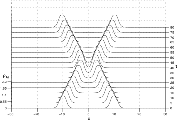
Figure 2: The time evolution of the charge density $\rho_{Q}$. $\Lambda_{l}=\Lambda_{r}=0.5$, $v_{l}=-v_{r}=0.2$, $x_{r}=-x_{l}=10$.

When two equal waves are at rest initially and with a phase shift of $\pi$, the results given in Fig. 3 show that they repulse fully each other. The repulsion force depends on their initial distance. The distance is smaller, the waves move faster in opposition. This phenomenon is different from the results on two waves in phase reported in [12], where the long-lived oscillating bound state is generated when $x_{r}=-x_{l}=3$.

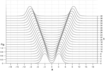
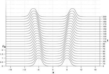
Figure 3: The time evolution of the charge density $\rho_{Q}$ for two initially resting, equal waves. Left: $\Lambda_{l}=\Lambda_{r}=0.6$, $x_{r}=-x_{l}=3$, right: $\Lambda_{l}=\Lambda_{r}=0.5$, $x_{r}=-x_{l}=6$.

Fig. 4 shows the computed results for the case of two unequal one-humped solitary waves. The left-hand plot is for the case of $\Lambda_{l}=0.6,\Lambda_{r}=0.8$, $v_{l}=-v_{r}=0.2$, and $x_{r}=-x_{l}=10$, and the right figure is for the case of $\Lambda_{l}=\Lambda_{r}=0.5$, $v_{l}=0.1,v_{r}=-0.9$, and $x_{r}=-x_{l}=10$. We see that the left-hand (or right-hand) initial solitary wave transfers charge and energy to the right-hand (or left-hand) one and the final solitary waves are moving with their initial velocities. Actually, we may consider that as a traversing or penetration phenomenon, that is to say, two waves go through each other in their interaction.

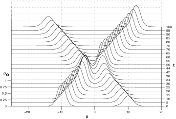
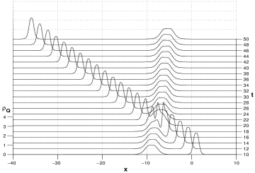
Figure 4: The time evolution of the charge density $\rho_{Q}$. Left: $\Lambda_{l}=0.6,\Lambda_{r}=0.8$, $v_{l}=-v_{r}=0.2$, $x_{r}=-x_{l}=10$; right: $\Lambda_{l}=\Lambda_{r}=0.5$, $v_{l}=0.1,v_{r}=-0.9$, $x_{r}=-x_{l}=10$.

We have conducted various different experiments on binary collisions of one-humped waves and concluded that in general collapse phenomenon cannot be observed in collisions between two one-humped waves. To save space, we do not give corresponding plots here.

3.2 Two two-humped solitary waves

This subsection is to study the interaction of two two-humped solitary waves with a phase shift of $\pi$.

Fig. 5 shows the computed results for the cases of $\Lambda_{l}=\Lambda_{r}=0.1$, $v_{l}=-v_{r}=0.2$ and $0.9$, and $x_{r}=-x_{l}=10$. We observe that the final solitary waves keep their initial velocities but with different shapes; the collapse does not happen in these both cases. It is worth noting that the collapse will happen if those two waves are in phase, see Fig. 2 in [13].

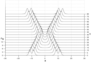
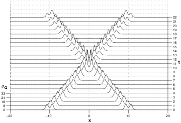
Figure 5: The time evolution of the charge density $\rho_{Q}$. $\Lambda_{l}=\Lambda_{r}=0.1$, $x_{r}=-x_{l}=10$. Left: $v_{l}=-v_{r}=0.2$; right: $v_{l}=-v_{r}=0.9$.

Consider the case of that two unequal waves are at rest initially and with a phase shift of $\pi$. The results given in Fig. 6 show that they repulse each other essentially, and the repulsion force depends on their initial distance. When two initial waves stand more nearly, the repulsion dominates in their interaction, thus they move outside fast and cannot re-collide each other, see the left figure in Fig. 6. But when the distance is relatively big, the right plot of Fig. 6 shows that two waves first repulse each other, then attract afterwards and collapse. When two initial waves are equal, at rest, and with a phase shift of $\pi$, we only observed full repulsion which is similar to that in the left figure of Fig. 6.

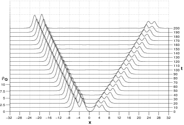
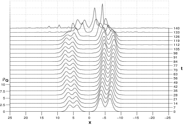
Figure 6: The time evolution of the charge density $\rho_{Q}$ for two initially resting waves. $\Lambda_{l}=0.1,\Lambda_{r}=0.2$. Left: $x_{r}=-x_{l}=4$; right: $x_{r}=-x_{l}=5$.

Besides the above, we also conduct some other experiments and find that collapse happens easily in collisions of two in-phase, equal, two-humped waves, but it may not appear in collisions between two in-phase, unequal, two-humped waves, or two equal two-humped waves with a phase shift of $\pi$, or two unequal, two-humped waves with a phase shift of $\pi$.

3.3 A one-humped solitary wave and a two-humped solitary wave

This subsection is to study the interaction of a one-humped solitary wave and a two-humped solitary wave, which are with a phase shift of $\pi$.

Fig. 7 shows the computed results for the case of $\Lambda_{l}=0.1,\Lambda_{r}=0.9$, $v_{l}=-v_{r}=0$, and $x_{r}=-x_{l}=6$. We see the quasi-stable long-lived oscillating bound state, which is essentially same as one shown in Fig. 3 in the paper [13]. Generally, when there is a big difference between the peak values of two initial waves, macroscopical behavior of the interaction dynamics are essentially independent on their phase shift.

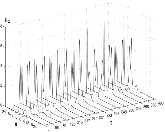
Figure 7: Bound state formed in binary collisions between two initially resting, out-of-phase waves. $\Lambda_{l}=0.1,\Lambda_{r}=0.9$, $v_{l}=v_{r}=0$, and $x_{r}=-x_{l}=6$.

Fig. 8 shows the computed results for the cases of $\Lambda_{l}=0.1,\Lambda_{r}=0.5$ and $0.9$, $v_{l}=-v_{r}=0.2$, and $x_{r}=-x_{l}=10$. It tells us that collapse may be observed in collisions between a one-humped solitary wave and a two-humped solitary wave when they do initially travel face to face, but it may also not happen.

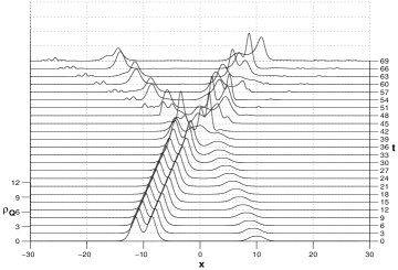
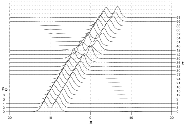
Figure 8: The time evolution of the charge density $\rho_{Q}$. $\Lambda_{l}=0.1$, $v_{l}=-v_{r}=0.2$, $x_{r}=-x_{l}=10$. Left: $\Lambda_{r}=0.5$; right: $\Lambda_{r}=0.9$.

4 Ternary collisions

In this section, we study ternary collisions by solving the nonlinear Dirac model (1) with the following initial data

$$\mbox{\boldmath$\psi$}(x,0)=e^{\mathrm{i}\theta_{l}}\mbox{\boldmath$\psi$}^{ss}_{l}(x-x_{l},0)+e^{\mathrm{i}\theta_{m}}\mbox{\boldmath$\psi$}^{ss}_{m}(x-x_{m},0)+e^{\mathrm{i}\theta_{r}}\mbox{\boldmath$\psi$}^{ss}_{r}(x-x_{r},0),$$ (15)

where $\theta_{l}$, $\theta_{m}$ and $\theta_{r}$ are three real numbers, determining the initial phase of corresponding waves.

The first case we consider is collisions of three initially resting two-humped solitary waves: $\Lambda_{l}=\Lambda_{m}=\Lambda_{r}=0.1$, $v_{l}=v_{m}=v_{r}=0$, $x_{r}=-x_{l}=10$, $x_{m}=0$, $\theta_{l}=\theta_{r}=0$, and $\theta_{m}=\pi$. The results are shown in Fig. 9. We see from the left plot that the waves first repulse each other because two neighboring waves are out-of-phase, but after $t=100$ they begin to attract each other, and final collision results in collapse. Symmetry of the solutions is kept very well. The right figure of Fig. 9 gives the charge and energy densities at $x=0$ as a function of time. We observe that before collapse happens, the middle wave is oscillating because of bind from left and right waves although its displacement seems to be unchanged.

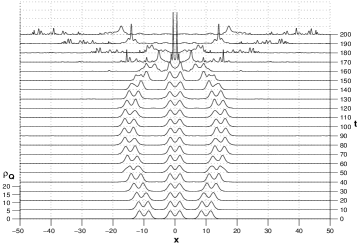
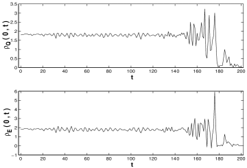
Figure 9: Collisions of three initially resting two-humped waves: $\Lambda_{l}=\Lambda_{m}=\Lambda_{r}=0.1$, $x_{r}=-x_{l}=10$, $x_{m}=0$, $\theta_{l}=\theta_{r}=0$, $\theta_{m}=\pi$. Left: plot of $\rho_{Q}(x,t)$; right: plots of $\rho_{Q}(0,t)$ and $\rho_{E}(0,t)$.

The second case is collisions of three initially resting one-humped waves: $\Lambda_{l}=\Lambda_{m}=\Lambda_{r}=0.5$, $v_{l}=v_{m}=v_{r}=0$, $x_{r}=-x_{l}=10$, $x_{m}=0$, $\theta_{l}=\pi$, and $\theta_{m}=\theta_{r}=0$. The results are shown in the left plot of Fig. 10. We see that the first interaction happens between two right in-phase waves around $t=45$, and then two faster moving waves are formed. The initially resting left wave begin to be moving towards left due to repulsion between it and the right waves, and then it is catched up with and interacted by the left moving wave generated in the first interaction around $t=130$. Overlapping happens in all two interactions. If we consider collisions of three initially resting one-humped waves with $\Lambda_{l}=\Lambda_{m}=\Lambda_{r}=0.6$ or 0.9, the interaction does only happen between two right neighboring in-phase waves, see the right plot of Fig. 10. The reason is that the left-moving (middle) wave formed in the interaction of two initially in-phase (right) waves is not faster than the left wave.

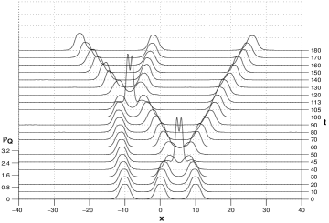
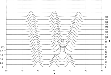
Figure 10: The time evolution of the charge density $\rho_{Q}$. $v_{l}=v_{m}=v_{r}=0$, $x_{r}=-x_{l}=10$, $x_{m}=0$, $\theta_{l}=\pi$, $\theta_{m}=\theta_{r}=0$. Left: $\Lambda_{l}=\Lambda_{m}=\Lambda_{r}=0.5$; right: $\Lambda_{l}=\Lambda_{m}=\Lambda_{r}=0.6$.

5 Discussions and Conclusions

In this paper, we further studied the interaction dynamics for the solitary waves of a nonlinear Dirac model (1) with scalar self-interaction. By using a fourth–order accurate RKDG method presented in [12], we investigated the interaction of the Dirac solitary waves with an initial phase shift of $\pi$ for the first time, and observed that: (a) full repulsion in binary and ternary collisions, and the initial distance between waves is smaller the repulsion is stronger; (b) repulsing first, attracting afterwards, and then collapse in binary and ternary collisions of two-humped waves; (c) interaction with one overlap and two overlaps in ternary collisions of initially resting waves, which depends on initial parameter $\Lambda$. We concluded that in general collapse phenomenon cannot be observed in collisions between one-humped waves, but it happens easily in collisions of in-phase, equal, two-humped waves; the macroscopical behavior of the interaction dynamics is essentially independent on their initial phase difference, when there is a big difference between the peak values of initial waves. Although we have investigated the influence of initial phase difference on the interaction dynamics of the Dirac solitary waves, it will be interesting and important to study the evolution of the relative phase of the solitons during their collisions.

References

- [1] M. Soler, Classical, stable, nonlinear spinor field with positive rest energy, Phys. Rev. D 1(1970), 2766-2769.
- [2] A.F. Raada, M. Soler, Perturbation theory for an exactly soluble spinor model in interaction with its electromagnetic field, Phys. Rev. D 8(1973), 3430-3433.
- [3] A.F. Raada, M.F. Raada, M. Soler, L. Vzquez, Classical electrodynamics of a nonlinear Dirac field with anomalous magnetic moment, Phys. Rev. D 10(1974), 517-525.
- [4] A. Alvarez, M. Soler, Energetic stability criterion for a nonlinear spinorial model, Phys. Rev. Lett. 50(1983), 1230-1233.
- [5] A. Alvarez, M. Soler, Stability of the minimum solitary wave of a nonlinear spinorial model, Phys. Rev. D 34(1986), 644-645.
- [6] A. Alvarez, Spinorial solitary wave dynamics of a (1+3)-dimensional model, Phys. Rev. D 31(1985), 2701-2703.
- [7] A. Alvarez and A. F. Rada, Blow-up in nonlinear models of extended particles with confined constituents, Phys. Rev. D 38(1988), 3330-3333.
- [8] A. Alvarez, B. Carreras, Interaction dynamics for the solitary waves of a nonlinear Dirac model, Phys. Lett. A 86(1981), 327-332.
- [9] A. Alvarez, Linearized Crank-Nicholson scheme for nonlinear Dirac equations, J. Comput. Phys. 99(1992), 348-350.
- [10] J. De Frutos, J.M. Sanz-serna, Split-step spectral schemes for nonlinear Dirac systems, J. Comput. Phys. 83(1989), 407-423.
- [11] Z.-Q. Wang, B.-Y. Guo, Modified Legendre rational spectral method for the whole line, J. Comput. Math. 22(2004), 457-474.
- [12] S.H. Shao, H.Z. Tang, Higher-order accurate Runge-Kutta discontinuous Galerkin methods for a nonlinear Dirac model, Discrete and continuous dynamical systems-series B 6(2006), 623-640.
- [13] S.H. Shao, H.Z. Tang, Interaction for the solitary waves of a nonlinear Dirac model, Phys. Lett. A, 345(2005), pp.119-128.