Form factor expansion for large graphs: a diagrammatic approach
Abstract.
The form factor of a quantum graph is a function measuring correlations within the spectrum of the graph. It can be expressed as a double sum over the periodic orbits on the graph. We propose a scheme which allows one to evaluate the periodic orbit sum for a special family of graphs and thus to recover the expression for the form factor predicted by the Random Matrix Theory. The scheme, although producing the expected answer, undercounts orbits of a certain structure, raising doubts about an analogous summation recently proposed for quantum billiards.
2000 Mathematics Subject Classification:
81Q50,34B45,15A521. Introduction
One of the central questions of quantum chaology is investigating which properties of the spectrum of a quantum system reflect the chaoticity of the underlying dynamics. It has been observed [BGS84] that if the classical limit is chaotic, the local statistical properties of the spectrum of a generic quantum system resemble those of the spectrum of a large matrix from a suitable random matrix ensemble. The choice of the ensemble depends only on very general characteristics of the system, such as whether it is time-reversal invariant, and whether spin is present. Clarifying the precise meaning of the term “generic” above and proving the conjecture of [BGS84] in any generality still remains one of the most exciting questions of quantum chaology.
Quantum graphs make ideal models to study the questions of quantum chaology, as they exhibit the same rich variety of behaviors and share the same set of analytical tools as the more complicated systems. However one can achieve deeper understanding on graphs while using methods which are simpler yet more rigorous. And due to direct analogies between graphs and more complicated systems like billiards and cavities, any advancement on graphs will provide insight to researchers in a much wider area. It is notable that some of the recent progress in understanding the role of periodic orbits in the spectral statistics was achieved on graphs first [BSW03, B04] and then extended to other systems [HMBH04].
In the present paper we aim to exploit the analogy between the tools used in quantum chaology on billiards and graphs to analyze a recent breakthrough result by Müller et al [MHBHA05]. The authors of [MHBHA05] investigate the form factor, one of the functions measuring the correlations within the spectrum of a classically chaotic quantum billiard. The advantage of the form factor lies in its convenient expansion in terms of pairs of periodic orbits of the classical system. This expansion is an application of the trace formulae (see [CPS98] for a review) and has been a starting point for many investigations. The progress in understanding the role of periodic orbits in the universal behavior of the form factor of billiard systems is marked by such milestones as the diagonal approximation [Ber85], the first off-diagonal contribution [Sie02, SR01] and, most recently, [MHBHA05] which announced a complete expansion of the form factor for the rescaled time . For quantum graphs, the corresponding steps have been taken in [KS97, KS99, Tan01] (the diagonal approximation) and [BSW02] (the first off-diagonal contribution). This article aims to lay the groundwork needed for the complete expansion. It must be mentioned that the form-factor for graphs has also been successfully analyzed using non-perturbative supersymmetric methods [GA04, GA05].
To introduce our results we need to briefly summarize the achievements of [MHBHA05]. Using an expansion of the form factor as a double sum over the periodic orbits of the classical system the authors classify the periodic orbit pairs and perform the summation to recover, for , the result predicted by the Random Matrix Theory. The summation can be loosely divided into two parts: evaluating the contribution of pairs of orbits related through a fixed transformation (described as a “diagram”) and summation of the resulting contributions over all possible transformations. While performing breathtaking (and mathematically rigorous) feats of combinatorics in the second part, the authors remain somewhat vague on the assumptions made about the ergodic nature of the periodic orbits in the first part. By analyzing the contributions of the diagrams on quantum graphs we aim to look for possible omissions in the derivation of [MHBHA05].
We are pleased to report that, in the large, we are able to replicate and thus confirm the findings of [MHBHA05]. In doing so, however, we are forced to omit a class of periodic orbits that do not fit well into the general summation. We believe that such orbits were also omitted (although less explicitly) in [MHBHA05]. These are the orbits with short stretches between the self-intersections. On one hand, if the conjecture of [BGS84] were to hold, such orbits should not contribute to the universal final answer: the short stretches are not universal. For exactly the same reason the task of dealing with such orbits is one of the hardest. A general method of proving that their contribution is negligible is badly needed for higher terms.
The paper is organized as follows: in section 2 we discuss the definition of the quantum graphs, their spectra, the relevant statistics, the trace formula and the particular model considered. Then we review the past results and difficulties encountered in section 3 and proceed to describe our new summation method in section 4. Our results are compared with those of Müller et al [MHBHA05] in section 5, where we also speculate about the possibility of periodic orbit summation beyond the Heisenberg time .
2. Spectral statistics of quantum graphs
2.1. Quantum dynamics on graphs
Here we will describe a general approach to quantization of a graph proposed by Schanz and Smilansky [SS99]. It shares many important features with another quantization procedure, used by several authors in the present volume (see, e.g., [kostrykin_schrader]), which is based on finding a self-adjoint extension of a second-order differential operator defined on the bonds of a graph. In particular, in many important cases (such as the Neumann boundary conditions) the resulting quantum spectra coincide.
We start with a graph where is a finite set of vertices (or nodes) and is the set of directed bonds (or edges). Each bond has a start vertex and an end vertex, they are specified via functions and . The start and end vertices specify a bond uniquely: we do not allow multiple edges. We will, however, consider graphs with looping bonds, i.e. such that . We demand that the set be symmetric in the sense that iff there is a bond such that and . The bond is called the reversal of . A looping bond acts as its own reversal. The operation of reversal is reflexive: . When we refer to the “non-directed bond ” we mean the couple of bonds, and . The number of vertices is denoted by and the number of directed bonds is . The vertices are usually marked by the integers starting from 0.
The graphs we will be considering are metric, that is each bond has a length denoted by . Naturally, . As a rule, we will be assuming that the different lengths are rationally independent, which means that the only choice of integers satisfying
| (1) |
is the trivial one: for all .
Now we define the quantum scattering map to be a unitary matrix
| (2) |
Here the matrix is diagonal with the elements , where is length of the bond . An element of the unitary matrix is zero unless the transition between and is possible according to the graph’s geometry (i.e. ). The evolution is defined by , where are -dimensional vectors of the wave amplitudes on the graph’s bonds. The eigenvalues of the system are the wavenumbers at which stationary solutions exist, i.e. has an eigenvalue one. The quantum evolution is time-reversal (TR) invariant if the elements of the matrix satisfy
| (3) |
The corresponding classical dynamics on the graph is defined as the Markov chain on the bonds of the graph with the transition matrix ,
| (4) |
One of the most exciting questions of quantum chaology on graphs is to relate the statistical properties of the spectrum of the quantum graph to the ergodic properties of the corresponding Markov chain.
2.2. Considered model
In this paper we will only consider a particular family of graphs, complete Fourier graphs. In a complete graph, there is a bond between any two vertices, including a loop from each vertex to itself. In a graph with vertices, is equal to . The corresponding matrix is defined by
| (5) |
where and are integers between 1 and . The distinguishing feature of a complete Fourier graph is the quick equilibration of the corresponding classical transition probability: the probability to go from a bond to a bond in steps is equal to independently of and as soon as .
2.3. Spectral statistics and the BGS conjecture
Consider an ordered sequence with mean density
| (6) |
equal to 1. The most popular quantity for numerical study of the statistical properties of the sequence is the nearest-neighbor spacing distribution, which is the weak limit (if it exists)
| (7) |
The two-point correlation function is a second order analogue of and is defined by
| (8) |
It is important to note that the normalization in front of the sum is and not , i.e. is not a probability distribution. The most popular quantity for analytical investigations is the Fourier transform of , the form factor,
| (9) |
It owes much of its popularity to its convenient representations via trace formulae.
Example 1.
Uncorrelated spectrum. Let be a sequence of independent exponentially distributed random variables with expectation 1. Define , these are the jump times of a Poisson process [Billingsley]. One can show that for the sequence , i.e. there are no detectable correlations within this sequence.
The Bohigas-Giannoni-Schmit (BGS) conjecture [BGS84], if applied to quantum graphs, claims that the spectrum of quantum graphs is correlated in the same way as in the spectrum of large random matrices [Mehta, Haake]. In the case of TR invariant quantum graphs, the random matrix should be from Gaussian Orthogonal Ensemble (GOE) or Circular Orthogonal Ensemble111Loosely speaking, GOE corresponds to the spectrum of the Hamiltonian whereas COE corresponds to the spectrum of the -matrix. The spectral statistics are the same. (COE). In particular, the form factor of graphs, should converge to the form factor for the Gaussian Orthogonal Ensemble (GOE),
| (10) |
as we increase the number of bonds . Since often there is no unique way of increasing the size of the graphs, a separate conjecture describes the sequences that are expected to produce convergence to the RMT statistics. This conjecture, often called the “Tanner conjecture” was formulated in [Tan01] (see also [GA04, GA05]); a related criterion was proposed in [BSW02, BSW03]. They can be summarized as requiring the mixing time of the Markov chain to grow sufficiently slowly with . Our model, the complete Fourier graphs, clearly satisfies this requirement: the mixing time is independent of .
2.4. Trace formula
One of the main links connecting a quantum system to the underlying dynamics is a trace formula which expresses the eigenvalues of the quantum system through a sum over the periodic orbits of the classical system. For quantum graphs the trace formula was established by Roth in [Roth83a, Roth83b] and rediscovered by Kottos and Smilansky in [KS97]. Before we can write it down, we need to give several definitions. Let be the set of all sequences
| (11) |
such that for any the bond follows the bond : (by we understand ). Define the cyclic shift operator on by
| (12) |
Equivalence classes in with respect to the shift are called periodic orbits of period . For a periodic orbit we define its length and amplitude by
| (13) |
correspondingly. A periodic orbit is a repetition if it can be represented as another orbit repeated times. The maximum of all such is called the repetition number and denoted . An orbit with is called prime. If is a prime number, all orbits of period are prime.
The trace formula establishes a connection between the set of all eigenvalues and the set of all periodic orbits ,
| (14) |
where is the sum of all bond lengths of the graph. The right-hand side of (14) is convergent in the sense of distributions. The trace formula is exact on quantum graphs and can be used to recover individual eigenvalues [BDJ02] as well as the whole density of states.
2.5. Eigenvalue vs eigenphase statistics
The trace formula, (14), provides a convenient expression for the form factor of eigenvalues ,
| (15) |
where (corresp. ) is a periodic orbit of length () and with “stability” amplitude (). As signified by the last Kronecker delta, two orbits and will contribute to the double sum only if the lengths of the orbits coincide.
It is even more convenient to consider the form factor of eigenphases of the graph’s scattering map. For a unitary operator, such as the matrix defined in (2), the form factor is defined at integer times by
| (16) |
where is the scaled time . In our case the averaging is performed either with respect to the lengths of individual bonds or with respect to . Both lengths and enter only via the matrix and averaging produces equivalent results. Expanding the powers of the trace we obtain
| (17) |
Substituting this into the definition of the form factor and performing the averaging we arrive to
| (18) |
It is an accepted fact222although the author is unaware of a mathematical proof of such a statement, the reasons behind this correspondence are discussed, among other sources, in [DS92, KS99, schanz] that it is equivalent to study the spectral statistics of the sequence of eigenvalues and the statistics of the eigenphases of . Certainly, if we send all individual bond lengths to in a fixed graph with real , it is clear from expressions (15) and (18) that will converge to in the sense of distributions on any compact interval.
We are interested in the limit of large graphs, , where is expected to converge to its limiting GOE form,
| (19) | |||||
When taking this limit we can ignore the orbits that are repetitions of other orbits, simplifying the formula for the form factor to
| (20) |
Equation (20) is the starting point for our derivation.
3. Past results
3.1. Diagonal approximation
To approach the task of evaluating the form factor one needs to classify possible pairs of orbits of equal length. The most simple such pair is and . Since we assumed that , we can also take to be the reversal of : . It turns out [Ber85] that such pairs provide the leading contributing term to the form factor, called the diagonal approximation. Evaluating it for graphs was studied in detail in [Tan01]. Here we recap the derivation of the diagonal approximation for our model, the complete Fourier graph, for which the number of directed edges is and the modulus square of amplitude of any orbit of period is .
| (21) |
Here we used the fact that there are asymptotically orbits on a complete graph (we divide by to take into account the shifts of the same orbit) and that the rescaled time is .
3.2. The difficulties in evaluating further corrections
To appreciate the difficulties present when evaluating off-diagonal corrections, it is instructive to consider the simplest first correction in some detail. The first correction comes from the Sieber-Richter pairs [SR01, Sie02], also called “figure of eight” orbits. We will say that an orbit has a self-intersection at vertex if there are indices and such that and , see Fig. 1. Then the “partner” orbit
| (22) |
will have the same length as (and it is easy to verify that the above is a legitimate orbit). We do not require that ; the general rule is that we reverse all the bonds starting with and until we have reversed .
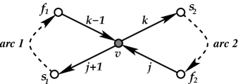
To evaluate the contribution of such pairs we need to introduce more terminology, summarized in Fig. 1. We will usually denote the intersection vertex by . The sequence of bonds we call arc 1; the sequence is arc 2. The starting vertex of arc 1, will be denoted , the end vertex . Similarly for the second arc, and . We define to be the contribution to the amplitude made by traversing arc ,
| (23) |
Using the above definition and the formula for we can write for and
| (24) | |||||
| (25) |
where is defined by appropriately reversing the bonds in . However, due to the reversal symmetry in the matrix , , we have . Therefore, the contribution of the pair to the form factor sum simplifies to
| (26) |
with the factorization in the exponent reminiscent of the expression for the action difference in billiard systems [Spe03, TR03].
It is now clear how one can sum over all “figure of eight” orbits. The sum will run over all possible intersection vertices, over possible choices for and and over possible configurations of arc 1 and 2 (including their length). This approach, however, is prone to counting orbits that should not be counted. There are two basic corrections.
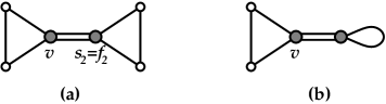
The first correction comes from the orbits in which , Fig. 2 (a). In this case the orbit runs along itself and one can use as another intersection point. It is clear, however, that this choice would produce the same partner orbit . A solution proposed in [BSW02] was to define the intersection point to be the leftmost vertex in such an “extended” intersection. In essence, this amounts to only counting the intersections with . This condition was called a restriction. In the present paper we modify this approach.
Another problem would arise if one of the arcs, say arc 2, was self-retracing. One of the simplest examples is when and arc 2 contains just one bond, a loop from to itself, Fig. 2 (b). In this case, reversing arc 2 would give back the same orbit and the pairing of with itself was already counted in the diagonal approximation. Such orbits were termed exceptions in [BSW02]; they were evaluated separately and subtracted from the previous result. We note that the previously imposed restriction means that there can be no exceptions with arc 1 being self-retracing. This shows that restrictions and exceptions cannot be treated independently. It should also be noted that both restrictions and exceptions must be treated carefully in order to get the correct result.
To find higher order terms, orbits fitting more complicated intersection patterns have to be considered. Diagrams were used in [BSW03] and [B04] to describe the relationship between the orbits and (i.e. which arcs get reversed). It proved to be hard to find and reconcile all the exceptions333We extend the notion of exceptions to denote all orbits that could fit a particular diagram but that were already counted in another diagram’s contribution and restrictions. We believe that the approach proposed in this paper helps to systematize the choice of restrictions in such a way that we avoid treating exceptions altogether. This approach was inspired by the recent work on billiard [MHBHA05]. It has its own shortcoming which will be discussed. We believe that this shortcoming applies to [MHBHA05] as well.
4. A consistent approach to evaluating diagrams
4.1. The second order diagram
We start by illustrating our approach on the simplest nontrivial diagram, the “figure of eight”. The trick is to introduce restrictions on both sides of the “extended” intersection and then sum over all possible intersection lengths, see Fig. 3.
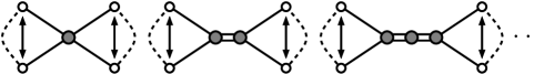
It turns out that we need to evaluate the first type of orbits on Fig. 3 separately. The contribution of such orbits reads
| (27) |
where we have implemented restrictions by using the Kronecker deltas. The term counts the number of ways to complete the orbit by choosing the arc configurations. The two arcs are uniquely defined by the vertices they pass through. Between the two of them, they pass through vertices (we have already chosen 6 vertices of the orbit: , , , , and twice). Thus there are ways to choose the lengths of the arcs and ways to choose the vertices themselves, leading to . Going back to (27), we open one of the brackets to obtain
| (28) | |||||
In both terms we perform the sum over . Since and , the first sum is identically 0. In the second we substitute throughout to get
| (29) | |||||
The obtained result is out of order: since , we got an answer of the order . Thus it is vital to evaluate the corrections from the extended intersections.
It is easy to see that for orbits with an extended intersection, is independent of the orbit configuration and is equal to . For an intersection of length , there are possible arc configurations. There are also ways to choose the vertices denoted by the shaded circles on Fig. 3 and ways to choose the vertices denoted by the empty circles. The total contribution is
The contribution of all “figure of eight” orbits is thus
| (30) |
Taking into account that , we recover the correct second-order correction . If we restrict the sum over to the values up to , we get a correction term of the form which decays faster than exponentially as we send and to infinity.
4.2. Evaluation of some third order diagrams
To gain some intuition for the general case we evaluate the contributions of two of the five diagrams contributing to the third order. The reader is referred to [BSW03] for a detailed list of the third order diagrams and their “multiplicities”. The treatment of these diagrams was also performed for disordered systems in [SLA98], and for chaotic billiards in [HMBH04].
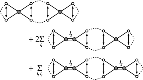
The first diagram we evaluate is the “sausage” orbits shown in Fig. 4. Here we need to require that all arcs (depicted by dashed lines) are at least one bond long. As noted by H. Schanz [schanz-private] this restriction excludes some potentially contributing orbits. Why they do not contribute to the form factor is a non-trivial question. In particular such orbits are not “rare” enough to guarantee a priori444by that we mean an estimate based on the number of orbits and the modulus of an orbit pair’s contribution, without taking into account the unitary cancellations that their contribution is vanishingly small. We conducted a separate study to evaluate the missing orbits for this particular diagram and discovered that cancellations akin to those in (30) ensure they do not contribute. However, we are not aware of any general argument applicable to higher diagrams.
In the intersections of length 0 (first and second line in Fig. 4) we open up one of the restrictions, in the same way as in (28). Another component necessary is the number of ways to complete the orbit by choosing the configurations of the 4 arcs. This is equal to , where
| (31) |
is the number of possible choices for the lengths of the arcs — essentially the number of partitions of into an ordered sum of 4 natural numbers. Now the total contribution of the diagram is
| (32) |
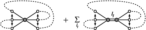
Next we evaluate a diagram with a triple intersection, shown in Fig. 5. The restrictions now mean that the three vertices cannot be all equal. In terms of Kronecker deltas it is implemented as . We again require that all arcs have non-zero bond lengths; this requirement excludes some orbits that ought to be counted. We must also note that in this case the restrictions do not fully rule out counting of orbits that ought to be excepted, for example the orbits with self-retracing arcs. The contributions of such orbits cannot be ruled out a priori — they occur often enough to contribute to the third order in . However they do not contribute (as signified by the results of [BSW03, B04]) due to cancellations which should be studied separately.
Turning a blind eye to these special orbits, we can evaluate the contributions of Fig. 5. There are now arc configurations, where
| (33) |
Dealing with case separately we arrive to
| (34) |
4.3. The general formula
The big advantage of the new way of evaluating diagrams is that the restrictions we impose essentially decouple different intersections from each other. This, in turn, allows us to write a general formula for a contribution of a diagram using only the information about the number of intersections and not how they are interconnected.
Consider the “sausage” diagram again. To write its contribution in a more uniform fashion we introduce a special factor, defined for ,
| (35) |
We can now rewrite the sums for in the following form:
| (36) |
where
In the first summand of (36), is a dummy variable since unless . In the second summand corresponds to in the second term of (32). Finally, in the third summand and counts the number of ways can be represented in such a way. Now we can generalize further by denoting by the number of 2-intersections in the diagram (in our case ) and by introducing the notation :
| (37) |
Using the same transformation, the contribution can be written as
| (38) |
where and . From here we generalize in the following fashion. Let, for a given diagram, the vector describe the number of intersections of multiplicities , etc. Let be the maximal multiplicity in the diagram: for . Then the contribution of this diagram is given by
| (39) |
where
We studied sum (39) for several values of and found that it gives the contribution derived in [MHBHA05],
| (40) |
where
At this point we can evoke the combinatorial results of [MHBHA05] for the number of diagrams with the characteristic . The summation of the leading order term of (40) over all possible diagrams then reproduces the predicted Random Matrix result, (10).
5. Conclusions, comparisons with [MHBHA05] and the outlook
In the present article we outline a construction which allows us to recover expression (40) for the contribution of a general diagram to the form factor of a complete Fourier quantum graph. The summation over all diagrams, described in [MHBHA05] would then recover the predicted Random Matrix result. However the final result, (39), was obtained at the cost of ignoring the orbits which can be generally characterized as having short stretches between self-intersections. We believe that the same omission was used in [MHBHA05], described in particular in the paragraph immediately following Eq.(16) (the discussion in Appendix D.2 is also relevant). While not claiming that the same applies to billiard systems, we can testify that on graphs the contribution of the orbits with very short stretches is absolutely divergent in the limit . This underlines the need to analyze the unitary cancellations which ensure that such orbits do not contribute to the final answer. The missing analysis also holds the key to the possibility of extending the discussed summation to systems with slower mixing.
Now that we have more understanding of how the universal contributions to the form factor arise from the sum of periodic orbits in the region , the question of why the expansion techniques break down beyond the Heisenberg time comes to the forefront. It seems, that if we are to recover the Random Matrix prediction for , the periodic orbit contributions would have to be classified in an entirely different way. Quite possibly, the summation needs to be based on the degeneracy classes — the sets of orbits of the same length — rather than on the diagram partition which is in a way transversal to the degeneracy class partition. Such degeneracy-based summation has been performed before for a special type of graphs, the Neumann star graphs [BK99] (see also [keating_here] for an overview of the results). The radius of convergence of the expansion was found to be finite but, if re-summed [BBK01], the result was valid for all values of . Important input for the question of going beyond can also be obtained by comparing the periodic orbit expansions with the non-perturbative methods of [GA04, GA05] which are valid for all .