Hexagonal, square and stripe patterns of the ion channel density in biomembranes

Abstract

Transmembrane ion flow through channel proteins undergoing density fluctuations may cause lateral gradients of the electrical potential across the membrane giving rise to electrophoresis of charged channels. A model for the dynamics of the channel density and the voltage drop across the membrane (cable equation) coupled to a binding-release reaction with the cell skeleton (P. Fromherz and W. Zimmerman, Phys. Rev. E 51, R1659 (1995)) is analyzed in one and two spatial dimensions. Due to the binding release reaction spatially periodic modulations of the channel density with a finite wave number are favored at the onset of pattern formation, whereby the wave number decreases with the kinetic rate of the binding-release reaction. In a two-dimensional extended membrane hexagonal modulations of the ion channel density are preferred in a large range of parameters. The stability diagrams of the periodic patterns near threshold are calculated and in addition the equations of motion in the limit of a slow binding-release kinetics are derived.

I Introduction

Spatio-temporal pattern formation is ubiquitous in systems driven away from thermal equilibrium CrossHo ; Cladis:95 ; Manneville:90 ; Murray:89 . Many physical, chemical and biological systems display dissipative structures, even though the underlying pattern forming mechanisms are often completely different. Nevertheless many of these patterns, especially those emerging at the primary bifurcation, belong to a few universality classes CrossHo and patterns occurring in rather disparate systems share qualitative and unifying properties.

Pattern forming processes in biological systems such as the fluid mosaic model, dilute filament-motor solutions (see e.g. Nedelec:1997.1 ; Kardar:2001.1 ; Liverpool:2003.2 ; Ziebert:2005.2 ), actively polymerizing filaments Ziebert:2004.1 , spiral waves in the cardiac system Panfilov:1995.1 , skin patterning of the angle fish Kondo:95.1 or oscillatory dynamics in cell division Mandelkow:89.1 ; Mandelkow:90.3 ; Hammele:2003.1 ; Kruse:2005.1 , are in general more elaborate than in classical pattern forming systems as for instance in fluid dynamics CrossHo . In the latter case the equations of motion can be derived by using elementary conservation laws and phenomenological transport laws and accordingly, for various patterns in fluid dynamical systems a quantitative understanding has been achieved with a high precision Cladis:95 ; CrossHo . These achievements can serve as a guide for the analysis of more involved biological or chemical pattern forming systems, where the respective models cover only the key steps of the complex biochemical reaction cycles.

In the present work we investigate pattern formation of ion channels embedded in a biomembrane. Membranes are an important building block of living cells and play a key role for the biological architecture. They consist of a lipid bilayer which is rather impermeable and build the barrier to the cell environment. All the vital components needed inside the cell are transported across membranes through specific proteins. Especially for the signal distribution along nerve cells (axons) the transport of ions through ion channels embedded in the membrane is essential since the transmembrane ion conductance is governed substantially by these discrete channels. The channel proteins are considered to move freely along the fluid lipid bilayer which is referred to as the fluid mosaic model Singer:72.1 , a concept that has attracted considerable attention. Describing the dynamics of ion channels within this framework, one finds transitions to various stationary as well as time-dependent density patterns with possible biological implications Fromherz:88.1 ; Fromherz:88.2 ; Fromherz:91.1 ; Fromherz:94.1 ; Zimmermann:95.2 ; SKramer:2002.1 ; Leonetti:2005.1 ; RPeter:2006.100 . The binding-release reaction removes the conservation of mobile ion channels and as a consequence causes pattern forming instabilities with a finite wave number. Accordingly one expects in two-dimensional extended systems beyond a stationary bifurcation either stripes, squares or hexagonal patterns as prototype patterns. Here we focus on the competition between these patterns in the presented model system.

Besides the fluid-mosaic model the channel concept Neher:76.1 is the second central physical idea in the field of biomembranes. It was found that including their electro-diffusion properties Jaffe:77.1 ; Stollberg:88.1 ; Nitkin:90.1 ion channels have an intrinsic propensity for self-organization Fromherz:88.1 . When a concentration gradient of salt across the membrane exceeds a certain threshold, the conserved number of freely movable ion channels may organize into transient periodic patterns which finally decay into global clusters Fromherz:88.2 ; Fromherz:91.1 ; Fromherz:94.1 .

The model of a fluid-mosaic of ion channels is only elementary and neglects at least three important properties of real biomembranes: (A) An interaction with signal molecules may induce a reversible molecular transition which opens or closes an ion channel Neher:76.1 , (B) an interaction with the cell skeleton may immobilize ion channels Poo:86.1 and (C) the excluded volume interaction between the ion channel molecules. The spatially dependent mobility of ion channels due to rafts Simons:1997a is also an effect neglected in the fluid mosaic model, but this heterogeneity effect is beyond the scope of the present work.

The opening-closing reaction keeps the number of mobile ion channels conserved and its effects on the instability of the homogeneous ion channel distribution have been investigated thoroughly in two recent publications SKramer:2002.1 ; RPeter:2006.100 . Since membrane deformations coupled to the underlying cell skeleton (actin cortex) may also open or close ion channels Aidley:96 ; Guharay:84.1 , additionally we take here both the immobilization and the closing of the channels into account Zimmermann:95.2 . For the sake of simplicity we choose a model which combines the two processes: We consider a reversible binding-release reaction of ion channels with the cell skeleton and assume that this interaction induces a closing of the channels. Alternative models for pattern formation along the cell membrane take additional intermediate steps of the opening-closing dynamics into account Fromherz:88.2 ; SKramer:2002.1 ; Korogod:2000.1 ; Leonetti:2005.1 but a thorough analysis of the pattern formation processes in two spatial dimensions is not available yet.

In the model we propose the closed ion channels which are considered to be bound to the cell skeleton are acting as a source for the mobile and open channels and therefore, the free and open ion channels are not conserved anymore in contrast to previously discussed models. We find in this model different kinds of selforganization of the mobile ion channels: With a considerable binding-release reaction one has an unconserved number of open channels and one finds (a) stable stripe or hexagonal patterns above threshold. This formation of stationary periodic patterns belongs to the same universality class as, for example, convection rolls in hydrodynamic systems. (b) The transition into the periodic pattern is either sub- or supercritical depending on the equilibrium constant, the relaxation time of the binding-release reaction and also on the strength of the excluded volume interaction of the ion channel molecules. In the limit of small binding-release reaction rates the model shows a crossover between pattern formation for an unconserved and a conserved order parameter. For this crossover regime a reduced equation is derived in Sec. IV.3.

This work is organized as follows: In Sec. II we describe the model system and we give the basic equations for the analysis in the subsequent sections. The linear stability of the homogeneous distribution of the ion channel density and the onset of the patterns is discussed in Sec. III. The amplitude equations, describing the weakly nonlinear behavior of stripes, hexagonal and square patterns are derived in Sec. IV. In this section also the nonlinear competition between these patterns is investigated by a thorough analysis. In Sec. V numerical solutions of the model equations are presented. Those numerical results provide an estimate for the validity range of the perturbational analysis given in Sec. IV. Concluding remarks and a discussion of the results are provided by Sec. VI.

II Model System

We consider a model membrane with embedded ion channels separating a thin electrolytic layer from an electrolytic bulk medium. This may refer to a cell membrane in close contact to another cell or to a membrane cable as it occurs in dendrites and axons of neurons. In the first case the thin layer is given by the extracellular cleft and the bulk by the cytoplasm. A particularly important biological example of this case is the post synaptic membrane of a neuronal synapse. In the second case the narrow cylindrical cytoplasm plays the role of a one-dimensional cleft opposed by the extracellular bulk medium.

Figure 1: A fluid membrane that separates a narrow cleft of electrolyte from a bulk electrolytic phase is considered. Membrane proteins are embedded in the lipid bilayer. They are mobile along the membrane (diffusion coefficient $D$), they form selective ion channels across the membrane (conductance $\Lambda$), they bear an electrophoretic charge $q$ and they interact with a filamentous substrate of the membrane (cell skeleton) via a binding-release reaction with rate constants $\kappa_{o}$ and $\kappa_{c}$. Binding closes the channels by a conformational change. The system is driven by a concentration gradient of those ions which are conducted by the channels (Nernst-type potential $E$). The model refers to the biological situations of a cell-cell-contact (post-synaptic membrane of a synapse) and of a cylindric cellular cable (neuron dendrites). The cleft of the model corresponds to the extracellular space in the first case, whereas it corresponds to the narrow cytoplasm in the second case. The structure of the model is described by the density of mobile channels $n({\bf r},t)$ and by the voltage in the cleft $v({\bf r},t)$ as a function of space ${\bf r}$ and time $t$.

Here we assume that the ion channels interact with the underlying cell skeleton, cf. Fig. 1 and Refs. Aidley:96 ; Guharay:84.1 ; Fromherz:91.2 . In a reversible binding-release reaction among the ion channels and the cell skeleton the ion channels undergo also a conformational change and switch between an opened and a closed state. This binding-release reaction of the ion channels (IC) is described by a simple reaction scheme with two rate constants $\kappa_{o}$ and $\kappa_{c}$, i.e. by an equilibrium constant $K_{BR}=\kappa_{o}/\kappa_{c}$ and a relaxation time $\tau_{BR}=(\kappa_{o}+\kappa_{c})^{-1}$:

$$IC^{bound}_{closed}\begin{array}[]{c}\kappa_{o}\\ \rightleftharpoons\\ \kappa_{c}\end{array}IC^{free}_{open}$$ (4)

The closed ion channels are bound to the cell skeleton and represent a source for free and open channels via the binding-release reaction. Accordingly the number of open and free channels is not conserved in our model, whereas in several previous investigations the number of free and open channels was conserved. Further mechanisms with similar consequences as the nonconservation of the ion channel number are also known Korogod:94.1 .

The free ion channels with an electrical conductance $\Lambda$ undergo a Brownian motion along the membrane with a diffusion coefficient $D$. They are selective for ions presenting a concentration gradient across the membrane which is described by a Nernst-type potential $E$. The proteins bear an effective electrophoretic charge $q$ leading to a drift motion in a lateral electrical field. The current through the mobile and open channels and through a homogeneous leak conductance of the membrane affects the local voltage in the cleft. In combination with an inhomogeneous distribution of the ion channels this gives rise to lateral gradients of the voltage.

II.1 Basic equations

In a mean field approximation the local density $n({\bf r},t)$ of free and open channels (particles per unit area) is determined by diffusion and electrophoretic drift of the ion channels, the binding-release reaction and the local interaction forces. The homogeneous density $\overline{n}$ is kept constant by a reservoir $\overline{n}_{c}=const.$ of bound channels by an equilibrium binding-release reaction given by Eq. (4) with $\overline{n}=K_{BR}\overline{n}_{c}$. The equations of motion for the channel density may be expressed in terms of the deviation

$$\tilde{n}=n-\overline{n}$$ (5)

from the mean density $\overline{n}$, where the dynamics is composed of a lateral current gradient and a source-sink contribution

$$\partial_{t}\tilde{n}\ =-\nabla\cdot{\bf j}(n)-\frac{\tilde{n}}{\tau_{BR}}\,.$$ (6)

The current depends on the part of the chemical potential, which is independent of the electric field, and on the mobility of the charged channels times the local electric field

$${\bf j}(n)=-\nabla\mu-\nu qn\nabla v$$ (7)

with the mobility

$$\nu=\frac{D}{k_{B}T}\enspace,$$ (8)

the diffusion constant $D$, the effective charge $q$ per channel, and the local voltage drop across the membrane $v({\bf r},t)$. The charge $q$ is assumed to be an effective charge taking into account screening as well as electro-osmotic effects Leonetti:1998.1 . The remaining part of the chemical potential may be derived from the free energy

$$\mu=\frac{\delta{\mathcal{F}}}{\delta\tilde{n}}\enspace,$$ (9)

where the free energy (per unit area S) of the channel-channel interaction is up to leading order in the deviation $\tilde{n}$ of the following from

$${\mathcal{F}}=\frac{1}{S}\int_{S}d{\bf r}\left[\,\frac{D}{2}\,{\tilde{n}}^{2}+\,\frac{g_{2}}{3}\,{\tilde{n}}^{3}+\,\frac{g}{4}\,{\tilde{n}}^{4}+\,\frac{1}{2}\xi^{2}(\nabla{\tilde{n}})^{2}\,\right]\,.$$ (10)

The higher order contributions become important especially for a negative diffusion constant $D$, if a demixing between lipid proteins and ion channels in the membrane takes place. Since the diffusion constant is assumed to be always positive for the present problem, the higher order contributions may be neglected in most situations. However, if the amplitudes of the spatial ion channel density modulations, as induced by the pattern forming mechanism discussed in this work, become strong, the second and third order terms in Eq. (10), describing the effects of excluded volume interactions become important in some range of parameters. Here we investigate exemplarily the stabilizing effects of the fourth order contribution to Eq. (10), i.e. with $g_{2}=0$, $\xi=0$ but $g\neq 0$. In this case the equation of motion for $\tilde{n}$ takes the following form

$$\partial_{t}\tilde{n}= \nabla^{2}\left(D{\tilde{n}}+g\tilde{n}^{3}\right)+\frac{qD}{k_{B}T}\,\nabla\cdot\left[\left(\tilde{n}+\overline{n}\right)\nabla v\right]-\,\frac{\tilde{n}}{\tau_{BR}}\,.$$ (11)

The voltage $v$ in the cleft is obtained from Kirchhoff’s law for each element of the membrane cable. Taking into account the current across the membrane and along the core of the cable or below a flat membrane, we obtain the Kelvin equation with the membrane capacitance $C$ either per unit length in a one dimensional model or per unit area for a two dimensional model, respectively, the resistance $R$ of the cleft per unit length (area) and the leak conductance $G$ of the membrane per unit length (area) Scott:75.1 ; Noble:1975

$$C\partial_{t}v=\frac{1}{R}\nabla^{2}v-G\,v-\Lambda n(v-E)\,.$$ (12)

The special case $\tau_{BR}\rightarrow\infty$ and $g=0$ of these equations has been investigated in Refs. Fromherz:88.1 ; Fromherz:91.1 ; Fromherz:94.1 .

II.2 Scaled Equations

We rescale Eq. (11) and Eq. (12) by introducing dimensionless coordinates for space ${\bf r}^{\prime}\,=\,{\bf r}/\lambda$ and time $t^{\prime}\,=\,t\,/\,\tau$ with the typical length scale of an electrical perturbation $\lambda\,=\,[R(\Lambda{\overline{n}}+G)]^{-1/2}$ and the time constant of displacement $\tau=\lambda^{2}/D$. We use normalized variables for the particle density $N=(n-\overline{n})/\overline{n}$ and voltage $V=(v-v_{R})q/k_{B}T$ with the resting voltage $v_{R}=\alpha E$ and the density parameter $\alpha=\Lambda\overline{n}/(\Lambda\overline{n}+G)$. Introducing the normalized relaxation time $\tau_{V}=RCD$ we obtain the normalized reactive Smoluchowski–Kelvin equations Leonetti:1998.1

$$\partial_{t^{\prime}}N= \nabla^{\prime 2}\left[N+gN^{3}\right]+\nabla^{\prime}\cdot\left[(1+N)\nabla^{\prime}V\right]-\beta N\,,$$ (13a)

$$\tau_{V}\partial_{t^{\prime}}V= \left[\nabla^{\prime 2}-1\right]V-\alpha(1-\alpha)\,\varepsilon N-\alpha NV\enspace.$$ (13b)

The dynamics of the system is controlled by the following three parameters: (i) The density parameter $\alpha$ characterizes the equilibrium of the binding-release reaction; (ii) the rate parameter $\beta=\tau/\tau_{BR}$ which characterizes the dynamics of the binding-release and the simultaneous opening-closing reaction; (iii) the control parameter $\varepsilon=-qE/(k_{B}T)$ which characterizes the distance to thermal equilibrium. Since the spread of the voltage is fast compared to the diffusion of ion channels ($R\approx 10^{8}\Omega,C\approx 1\mu F/cm^{2},D\approx 0.1\mu m^{2}/s\rightarrow\tau_{v}\ll 1$ Hille:92 ) we put $\tau_{V}=0$ in the following. For simplicity the primes of the new coordinates ${\bf r}^{\prime}$ and $t^{\prime}$ are suppressed further on.

III The onset of periodic patterns

The onset of spatial patterns takes place in a parameter range, where the homogeneous density $n=\overline{n}$ of the mobile channels, i.e. $N=0$ and $V=0$, becomes linearly unstable with respect to small inhomogeneous perturbations. In order to calculate this instability the linear part of Eqs. (13) is transformed by an ansatz

$$\left(\begin{array}[]{c}N\\ V\end{array}\right)=\left(\begin{array}[]{c}\delta\!N\\ \delta\!V\end{array}\right)e^{\sigma t+i{\bf k}{\bf r}}$$ (18)

into linear algebraic equations. The solubility condition of these equations determines for finite perturbations $\delta N,~{}\delta V\not=0$ and for $\tau_{V}=0$ the dispersion relation $\sigma(k)$

$$\sigma=-k^{2}\left(1-\frac{\alpha(1-\alpha)\varepsilon}{1+k^{2}}\right)-\beta\,\,$$ (19)

with $k=|{\bf k}|$, which is shown for three different values of the control parameter $\varepsilon$ in Fig. 2(a). A perturbation grows in the range of the wave number $k$ where the real quantity $\sigma(k)$ becomes positive. The neutral stability condition $\sigma(k)$=0 applied to the expression in Eq. (19) gives the neutral curve as follows

$$\varepsilon_{0}(k)=\frac{1+k^{2}}{\alpha(1-\alpha)}\,\left(1+\frac{\beta}{k^{2}}\right)\,,$$ (20)

where $\varepsilon_{0}(k)$ separates the range of stable from the unstable parameter values. A set of neutral curves $\varepsilon_{0}(k;\alpha,\beta)$ is shown in Fig. 2(b) for different values of the rate parameter $\beta$.

The minimum of $\varepsilon_{0}(k;\alpha,\beta)$ defines the critical wave number

$$k_{c}=\beta^{\frac{1}{4}}$$ (21)

and the critical control parameter

$$\varepsilon_{c}=\frac{\left(1+\sqrt{\beta}\right)^{2}}{\alpha(1-\alpha)}$$ (22)

at which the basic state becomes first unstable.

Figure 2: Part (a) shows the dispersion relation $\sigma(k)$ as given by Eq. (19) for a supercritical, a critical and subcritical value of the reduced control parameter $\eta$ and for the rate parameter $\beta=0.08$. Part (b) shows for four different values of the rate parameter $\beta=0.01,0.1,0.5,1.0$ (bottom to top) the neutral curves $\alpha(1-\alpha)\varepsilon_{0}(k)$ (solid lines) with $\varepsilon_{0}(k)$ given by Eq. (20). The dashed curve in (b) marks the location of the minimum of these neutral curves, i.e. the critical wave number $(k_{c},\varepsilon_{c})\,(\beta)$ as given by Eq. (21) and Eq. (22).

For $\varepsilon$-values above the neutral curve $\varepsilon_{0}(k,\alpha,\beta)$ the growth rate $\sigma$ is positive and it takes its maximum at the wave number $k_{m}$

$$k_{m}^{2}=-1+\left(1+\sqrt{\beta}\,\right)\,\sqrt{1+\eta}\,,$$ (23)

whereby the reduced control parameter $\eta$

$$\eta=\frac{\varepsilon-\varepsilon_{c}}{\varepsilon_{c}}\,\,$$ (24)

has been introduced. For a vanishing rate parameter $\beta=0$ the number of channels is conserved and the dispersion in Eq. (19) is at small values of $k$ proportional to $k^{2}$ which is similar to hydrodynamic excitation modes. To some extent this limit has already been investigated previously Fromherz:88.1 ; Fromherz:88.2 ; Fromherz:91.1 .

IV Weakly nonlinear analysis

For a finite value of the binding-release reaction parameter $\beta$ the fraction of the open ion channels is not conserved. In addition the homogeneous distribution of the ion channel density as well as the homogeneous voltage drop across the membrane may become simultaneously unstable against perturbations above a certain threshold. The perturbation with the wave number $k_{c}=\beta^{1/4}$ has the largest growth rate, as described in the previous section.

Near threshold and in two spatial dimensions this periodic instability may lead to stripe, square and, if the up-down symmetry is broken, also to hexagonal patterns CrossHo . In a parameter range where the amplitudes of these patterns are still small, the slow spatial variations of these patterns may be described in terms of generic amplitude equations, a method used for many other physical, chemical and biological pattern forming systems CrossHo ; Newell:92.1 . These generic equations and their corresponding functionals are derived in this section from the present model system whereby the detailed scheme of derivation is given exemplarily for stripes in App. A. The parameter ranges where each pattern realizes the lowest functional value and where two patterns coexist are determined in Sec. IV.2. Far beyond the threshold the solutions are determined numerically and the question of preference of patterns is addressed by numerical simulations in Sec. V.

In the range where the binding-release reaction becomes rather slow and the number of channels nearly conserved, i.e. $\beta\propto\eta^{2}$, another set of equations is derived and discussed in part IV.3. The analytical solutions derived in the two cases $\beta\propto O(1)$ and $\beta\propto\eta^{2}$ are compared with numerical solutions of Eqs. (13) in Sec. V.

IV.1 Periodic patterns for a finite binding-release reaction, $\beta\propto O(1)$

IV.1.1 Stripe patterns

For finite values of $\beta$ the solution of the linear part of Eqs. (13) is in the simplest case spatially periodic in one direction. The two fields $N$ and $V$ may be written as a vector ${\bf u}=\left(N,V\right)$ in the form

$${\bf u}_{0}={\bf\hat{e}}_{0}\,A\,e^{i{\bf k}_{c}{\bf r}}+c.c.$$ (25)

with the eigenvector

$${\bf\hat{e}}_{0}=\left(\begin{array}[]{c}1\\ E_{0}\end{array}\right),\quad E_{0}=-\left(1+\sqrt{\beta}\right)$$ (28)

where c.c. denotes the complex conjugate of the preceding term. Due to rotational symmetry the orientation of the wave vector

$${\bf k}_{c}=k_{c}\left(\begin{array}[]{c}1\\ 0\end{array}\right)$$ (31)

may be chosen parallel to the x-direction. Spatial variations of the pattern which are slow on the length scale $2\pi/k_{c}$, are described in Eq. (25) by a spatially dependent amplitude $A(x,y,t)$. The evolution equation for this spatially and time dependent amplitude is a so-called amplitude equation, namely the Ginzburg-Landau equation in our case, which takes for an isotropic two-dimensional system, as for instance for the two-dimensional flat membrane, the following universal form Newell:92.1 ; Manneville:90 ; CrossHo :

$$\tau_{0}\partial_{t}A=\left[\eta+\xi_{0}^{2}\left(\partial_{x}-\frac{i}{2k_{c}}\partial_{y}^{2}\right)^{2}-\gamma|A|^{2}\right]A\,.$$ (32)

The values of the coefficients $\tau_{0}$, $\xi_{0}$ and $\gamma$ depend on the specific pattern forming system Manneville:90 ; CrossHo ; Zimmermann:91.1 . The relaxation time $\tau_{0}$ and the coherence length $\xi_{0}$ in the amplitude equation (32) may be derived from the dispersion relation $\sigma(k)$ in Eq. (19) and from the neutral curve $\varepsilon_{0}(k)$ specified in Eq. (20) by a Taylor expansion of both formulas around the critical point $(k_{c},\varepsilon_{c})$ (see for instance Refs. Brand:86.1 ; CrossHo ; Zimmermann:93.1 ):

$$\tau_{0}^{-1} =\left.\frac{\partial\sigma}{\partial\varepsilon}\right|_{\varepsilon=\varepsilon_{c}}\,\varepsilon_{c}~{}, \xi_{0}^{2} =\frac{1}{2\varepsilon_{c}}\frac{\partial^{2}\varepsilon_{0}}{\partial k^{2}}\,.$$ (33)

Using the expressions in Eq. (19) and Eq. (20) we obtain their explicit form for the present model:

$$\tau_{0} =\frac{1}{\sqrt{\beta}\left(1+\sqrt{\beta}\right)}\,, \xi_{0}^{2} =\frac{4}{\left(1+\sqrt{\beta}\right)^{2}}\,.$$ (34)

The sign of the nonlinear coefficient $\gamma$ determines, whether the transition to the periodic state as described by Eq. (25) is supercritical ($\gamma>0$) or subcritical ($\gamma<0$), and it may be derived by a perturbation calculation from the basic equations (13):

$$\gamma= \frac{3g}{1+\sqrt{\beta}}-\frac{1}{3}\Biggl{[}\,\frac{6\alpha^{2}-\left(2+2\sqrt{\beta}-\alpha\right)^{2}}{1+\sqrt{\beta}}$$ (35)

$$\quad+\frac{2}{3\sqrt{\beta}}\left(4\sqrt{\beta}-2\alpha+1\right)\left(\sqrt{\beta}-2\alpha+1\right)\,\Biggr{]}\,.$$

The common scheme for the derivation of $\gamma$ may be found for instance in Refs. CrossHo ; Newell:92.1 ; Zimmermann:93.1 and the details of this calculation for the present system are given in App. A.

The linear coefficients in Eq. (34) depend only on the rate parameter $\beta$. By increasing the binding-release reactions the relaxation time and also the correlation length becomes smaller. The nonlinear coefficient depends besides the rate parameter $\beta$ also on the density parameter $\alpha$ and on the nonlinear interaction parameter $g$. In the limit $\beta\to 0$ for $\alpha\neq 1/2$ the relaxation time $\tau_{0}$ and the nonlinear coefficient $\gamma$ diverge. This behavior reflects the fact that in this limit the validity range of the amplitude equation is left and a different perturbation expansion has to be used as described in Sec. IV.3 below.

The amplitude equation (32) for a stripe solution can also be derived from a functional ${\mathcal{F}}$

$$\tau_{0}\partial_{t}A=-\frac{\delta{\mathcal{F}}_{S}}{\delta A^{\ast}}\,,$$ (36)

($A^{\ast}$ denotes the complex conjugate of $A$) of the following form

$${\mathcal{F}}_{S}=\frac{1}{S}\int_{S}d{\bf r}\left[\frac{\gamma}{2}|A|^{4}-\eta|A|^{2}+\xi_{0}^{2}\left|\left(\partial_{x}-\frac{i}{2k_{c}}\,\partial_{y}^{2}\right)A\right|^{2}\right].$$ (37)

In the following we will focus on spatially homogeneous patterns and their competition, i.e. $A(x,t)\rightarrow A(t)$. So the Ginzburg-Landau equation (32) reduces to a Landau equation

$$\tau_{0}\partial_{t}A=\eta A-\gamma|A|^{2}A$$ (38)

with a simplified functional

$${\mathcal{F}}_{S}=\frac{1}{S}\int_{S}d{\bf r}\left[\frac{\gamma}{2}|A|^{4}-\eta|A|^{2}\right]=\frac{\gamma}{2}|A|^{4}-\eta|A|^{2}\,.$$ (39)

Besides the trivial solution $A=0$, Eq. (38) has a second stationary solution

$$A=\sqrt{\frac{\eta}{\gamma}}\,.$$ (40)

This solution exists in the supercritical case $\gamma>0$ only above the threshold and for $\gamma<0$ only in the range $\eta<0$ on the unstable branch of the subcritical bifurcation. As the herein presented expansion breaks down for subcritically bifurcating stripes, higher order terms with respect to $A$ would have to be taken into account in order to achieve a limitation of the amplitude $A$ which may however be determined by solving Eqs. (13) beyond threshold numerically as done in Sec. V.

The parameter range of the supercritical and subcritical bifurcation are separated by the tricritical line $\gamma(\alpha,\beta)=0$. This line is shown in Fig. 3 in the $\alpha-\beta$ plane for different values of the excluded volume parameter $g$, where the supercritical range may be extended by increasing the nonlinear parameter $g$.

Figure 3: The lines describe the tricritical point, i.e. $\gamma(\alpha,\beta,g)=0$, for the stripe pattern in the $\alpha-\beta$ plane and for different values of the interaction coefficient $g$, respectively. On the right hand side of each curve corresponding to different values of $g$, $\gamma$ is positive and stripes bifurcate supercritically.

In the limit $\beta\to 0$ and $\alpha\to 1/2$ the nonlinear coefficient $\gamma=3g+1/4>0$ is positive and the bifurcation still supercritical. Otherwise $\gamma$ diverges in the limit $\beta\to 0$. This is also in agreement with an alternative perturbation analysis as described in Sec. IV.3.

IV.1.2 Square patterns

Square patterns can be described by a superposition of two periodic waves as given by Eq. (25)

$${\bf u}_{0}={\bf\hat{e}}_{0}\, \left(A_{1}e^{i{\bf k}_{1}{\bf r}}+A_{2}e^{i{\bf k}_{2}{\bf r}}\right)+c.c.\,,$$ (41)

whereby the two wave vectors ${\bf k}_{1}$ and ${\bf k}_{2}$ have the same length but both are orthogonal to each other

$${\bf k}_{1}=k_{c}\left(\begin{array}[]{c}1\\ 0\end{array}\right)\quad{\rm and}\quad{\bf k}_{2}=k_{c}\left(\begin{array}[]{c}0\\ 1\end{array}\right)\,.$$ (46)

Similar as for stripes, one may derive by a perturbation calculation from the basic Eqs. (13) the following two coupled equations for the two amplitudes $A_{1}$ and $A_{2}$

$$\tau_{0}\partial_{t}A_{1}= \,\eta\,A_{1}-\left(\gamma\,|A_{1}|^{2}+\chi\,|A_{2}|^{2}\right)A_{1}\,,$$ (47a)

$$\tau_{0}\partial_{t}A_{2}= \,\eta\,A_{2}-\left(\gamma\,|A_{2}|^{2}+\chi\,|A_{1}|^{2}\right)A_{2}\,,$$ (47b)

wherein the spatial dependence of the amplitudes has already been discarded. Herein $\tau_{0}$ and $\gamma$ are defined by the same expressions as for stripes in Eq. (34) and Eq. (35). For squares one obtains with a perturbation calculation, similar as described in App. A, the same expression for $\gamma$ as in Eq. (35) and the nonlinear coupling term $\chi$

$$\chi= -4\left(2(1-2\alpha)+\sqrt{\beta}\right)$$ (48)

$$+\frac{2\left(3g+\alpha^{2}-2(1-2\alpha)^{2}\right)}{1+\sqrt{\beta}}-\frac{4(1-2\alpha)^{2}}{\sqrt{\beta}(1+\sqrt{\beta})}\enspace.$$ (49)

As for stripes, the two coupled equations may be once again be derived from a functional

$$\tau_{0}\partial_{t}A_{i}=-\frac{\delta{\mathcal{F}}_{Q}}{\delta A_{i}^{*}}$$ (50)

by determining the extremal value of the functional

$${\mathcal{F}}_{Q}=\sum_{i=1}^{2}\left(\frac{\gamma}{2}\,|A_{i}|^{4}-\eta\,|A_{i}|^{2}\right)+\chi|A_{1}|^{2}\,|A_{2}|^{2}\,.$$ (51)

Apart from the trivial solution $A_{1}=A_{2}=0$, the coupled amplitude equations $(\ref{amplisquare})$ have two types of stationary solutions of finite amplitudes. The first type corresponds to simple stripe solutions with only one finite modulus

$$|A_{1}|=\sqrt{\frac{\eta}{\gamma}}~{},\,|A_{2}|=0\quad{\rm or}\quad|A_{1}|=0~{},\,|A_{2}|=\sqrt{\frac{\eta}{\gamma}}~{}\,.$$ (52)

For the second type of solutions the amplitudes have identical moduli

$$|A_{1}|=|A_{2}|=\sqrt{\frac{\eta}{\gamma+\chi}}$$ (53)

which corresponds to a square pattern as can be seen from Eq. (41).

If the sum of the two nonlinear coefficients is positive, i.e. $\gamma+\chi>0$, a square pattern bifurcates supercritically from the homogeneous state. A vanishing sum $\gamma+\chi=0$ marks the tricritical line of the square pattern, the bifurcation changes from a supercritical to a subcritical one. The tricritical line is displayed for different values of the interaction parameter $g$ in Fig. 4, where increasing values of $g$ broaden also the range of supercritically bifurcating squares in the $\alpha-\beta$ plane.

Figure 4: The nonlinear coefficient $\gamma+\chi$ as given by Eq. (48) is positive and square pattern bifurcate supercritically in the range enclosed by the solid line for $g=0.0$, for $g=0.1$ in the range enclosed by the dashed line and for $g=0.5$ between the dotted line.

IV.1.3 Hexagonal patterns

In two-dimensional systems close to the threshold and without an up-down symmetry $N,V\to-N,-V$ as in the Eqs. (13) hexagonal structures are often preferred in some parameter range to stripe or square patterns CrossHo . In this section the amplitude equations of hexagons are presented as they result by a perturbation calculation from Eqs. (13) similar as described in App. A for stripes.

Close to threshold a hexagonal pattern can be described by a superposition of three plane waves (stripe patterns) as given by Eq. (25), but where the three wave vectors enclose an angle of $2\pi/3$ with respect to each other. The solution may thus be represented by

$${\bf u}_{0}={\bf\hat{e}}_{0}\left(A_{1}e^{i{\bf k}_{1}{\bf r}}+A_{2}e^{i{\bf k}_{2}{\bf r}}+A_{3}e^{i{\bf k}_{3}{\bf r}}\right)+c.c.\,,$$ (54)

whereas the wave vectors ${\bf k}_{i}$ ($i=1,2,3$) are given by

$${\bf k}_{1}=k_{c}\left(\begin{array}[]{c}1\\ 0\end{array}\right)\quad{\rm and}\quad{\bf k}_{2,3}=\frac{k_{c}}{2}\left(\begin{array}[]{c}-1\\ \pm\sqrt{3}\end{array}\right)\,.$$ (59)

The coupled amplitude equations for the three envelope functions $A_{i}$ ($i=1,2,3$) are of the following form

$$\tau_{0}\partial_{t}A_{1}= \,\eta\,A_{1}+\delta\,A_{2}^{*}A_{3}^{*}$$

$$\quad-\left(\gamma\,|A_{1}|^{2}+\rho\,|A_{2}|^{2}+\rho\,|A_{3}|^{2}\right)A_{1}\,,$$ (60a)

$$\tau_{0}\partial_{t}A_{2}= \,\eta\,A_{2}+\delta\,A_{3}^{*}A_{1}^{*}$$

$$\quad-\left(\gamma\,|A_{2}|^{2}+\rho\,|A_{3}|^{2}+\rho\,|A_{1}|^{2}\right)A_{2}\,,$$ (60b)

$$\tau_{0}\partial_{t}A_{3}= \,\eta\,A_{3}+\delta\,A_{1}^{*}A_{2}^{*}$$

$$\quad-\left(\gamma\,|A_{3}|^{2}+\rho\,|A_{1}|^{2}+\rho\,|A_{2}|^{2}\right)A_{3}\,,$$ (60c)

with $A_{i}^{*}$ being the complex conjugate of $A_{i}$. $\tau_{0}$ and $\gamma$ are defined by the same expressions as for stripes and squares above in Eq. (34) and Eq. (35) and the two nonlinear coupling constants $\delta$ and $\rho$ read within the scope of our model system

$$\delta= \frac{1+\sqrt{\beta}-2\alpha}{1+\sqrt{\beta}}\,,$$ (61a)

$$\rho= \frac{6g}{1+\sqrt{\beta}}-\frac{4\alpha^{2}}{(1+\sqrt{\beta})^{3}}+\frac{2\alpha(1+\alpha)}{(1+\sqrt{\beta})^{2}}-\frac{3(2+\sqrt{\beta})}{4(1+\sqrt{\beta})}$$

$$-\frac{(1-2\alpha)(3+2\alpha)}{4\sqrt{\beta}(1+\sqrt{\beta})}+\frac{2\alpha(1-2\alpha)}{\sqrt{\beta}}+3\alpha\,.$$ (61b)

These three coupled nonlinear equations (60) may again be derived via the relation

$$\tau_{0}\partial_{t}A_{i}=-\frac{\delta{\mathcal{F}}_{H}}{\delta A_{i}^{*}}$$ (62)

from a functional

$${\mathcal{F}}_{H}= \sum_{i=1}^{3}\left(\frac{\gamma}{2}\,|A_{i}|^{4}-\eta\,|A_{i}|^{2}\right)+\frac{\rho}{2}\sum_{i\neq j}^{3}|A_{i}|^{2}\,|A_{j}|^{2}$$

$$\qquad\qquad-\delta\,\left(A_{1}A_{2}A_{3}+A_{1}^{*}A_{2}^{*}A_{3}^{*}\right)\,.$$ (63)

Eqs. (60) admit two types of homogeneous solutions. The first one corresponds to a stripe solution with only one non-vanishing amplitude. For hexagonal solutions the moduli of the three amplitudes $|A_{1}|=|A_{2}|=|A_{3}|=A$ coincide, but if one allows still a relative phase shift $\phi_{i}$ ($i=1,2,3$), with

$$A_{i}=A\,e^{i\phi_{i}}\,,$$ (64)

one obtains the nonlinear equation

$$0=\eta A+\delta\,e^{i\Phi}A^{2}-(\gamma+2\rho)A^{3}\,,$$ (65)

with the sum of the three phase angles $\Phi=\phi_{1}+\phi_{2}+\phi_{3}$. There are two real solutions of Eq. (65)

$$A_{\pm}=\frac{1}{2(\gamma+2\rho)}\left[\delta\pm\sqrt{\delta^{2}+4\eta\left(\gamma+2\rho\right)\,\,}\right]\,,$$ (66)

with $A_{+}$ corresponding to the larger amplitude for $\delta>0$ and $A_{-}$ for $\delta<0$. For $\delta>0$ the phase angle is $\Phi=0$, which corresponds to regular hexagons and for $\delta<0$ the angle is $\Phi=\pi$, which corresponds to inverse hexagons. Comparing for both solutions the functional ${\mathcal{F}}^{\pm}$ given by Eq. (IV.1.3), one finds that regular hexagons have the lower functional, i.e. ${\mathcal{F}}_{H}^{+}<{\mathcal{F}}_{H}^{-}$, in the range with $\delta>0$ and inverse hexagons in the range of $\delta<0$ with ${\mathcal{F}}_{H}^{+}>{\mathcal{F}}_{H}^{-}$.

The bifurcation from the homogeneous distribution of ion channels to a hexagonal modulation of the channel density is subcritical according to the quadratic nonlinearity $A^{2}$ in Eq. (65), which originates from the quadratic nonlinearity $A^{\ast}_{i}A^{\ast}_{j}$ in Eqs. (60). However, the amplitudes $A_{i}$ are still bounded by cubic nonlinearities in the parameter range of a positive nonlinear coefficient $\gamma+2\rho>0$ in Eq. (65). This nonlinear coefficient vanishes along the lines shown for different values of the parameter $g$ in the $\alpha-\beta$ plane in Fig. 5. If this coefficient becomes negative, i.e. $\gamma+2\rho<0$, Eqs. (60) do not have any stationary, finite amplitude solutions. In this case one needs either a higher order expansion or the amplitudes of hexagons have to be determined by solving the basic equations (13) numerically. Increasing values of the nonlinear interaction parameter $g$ enlarges the parameter range wherein stationary solutions of the form (66) occur.

Figure 5: The nonlinear coefficient $\gamma+2\rho$ for hexagons is positive between the solid line for $g=0.0$, for $g=0.1$ between the dashed line and for $g=0.5$ between the dotted line. In each range the amplitude of the hexagonal solution is limited by the cubic terms in Eq. (60).

IV.2 Competition between patterns

In the shaded subrange in Fig. 6 stripes and squares bifurcate both supercritically and the amplitude of the hexagons is simultaneously limited by a cubic term. This range becomes even larger with increasing values of $g$ as indicated by the ranges in Fig. 3, Fig. 4 and Fig. 5. So the interesting question arises, which of the three solutions is preferred in this overlapping range.

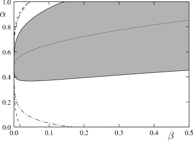
Figure 6: The bifurcation behavior of stripes, squares and hexagons is shown in the $\alpha$-$\beta$ plane for $g=0.5$: In the shaded range the amplitudes for stripes, squares and hexagons are limited by a cubic nonlinearity, i.e. $\gamma>0$, $\gamma+\chi>0$ and $\gamma+2\rho>0$. On the right hand side of the dashed line, which is determined by $\gamma=0$, stripes bifurcate supercritically and squares do so in the range inclosed by the solid line, which is defined by $\gamma+\chi=0$. Between the dashed-dotted line which is determined by $\gamma+2\rho=0$ hexagons are limited by cubic order terms.

One criterion is the comparison of the values of the functionals, i.e. to which solution belongs the lowest value of the respective functional ${\mathcal{F}}$. The second criterion is the linear stability of each of the nonlinear solutions, i.e. in which subrange of the overlap range of parameters becomes one of the solutions linear unstable with respect to small perturbations.

IV.2.1 Comparison of the functionals for stripes, squares and hexagons.

For one set of parameters, $\beta=0.15$, $\eta=0.06$ and $g=0.5$, the functionals of the three patterns are shown in Fig. 7 as a function of $\alpha$ in the range where each of them bifurcates supercritically. This figure indicates, in which region the respective pattern has the lowest value of the functional.

Figure 7: The functional ${\mathcal{F}}$ per unit area is shown for stripes (${\mathcal{F}}_{S}$), squares (${\mathcal{F}}_{Q}$), regular (${\mathcal{F}}_{H}^{+}$) and inverse hexagons (${\mathcal{F}}_{H}^{-}$) as a function of the parameter $\alpha$ as well as for the parameter values $\beta=0.15$, $\eta=0.06$ and $g=0.5$.

For small ($\alpha<0.49$) and very large values of $\alpha$ ($\alpha>0.98$) the functional ${\mathcal{F}}_{Q}$ has the lowest value, i.e. squares have the lowest energy and are accordingly preferred. Regular hexagons ${\mathcal{F}}_{H}^{+}$ are preferred in the range $0.49<\alpha<0.56$, stripes ${\mathcal{F}}_{S}$ in the range $0.56<\alpha<0.86$ and finally inverse hexagons ${\mathcal{F}}_{H}^{-}$ in the range $0.86<\alpha<0.98$. These respective ranges change as a function of $\eta,\,\beta$ and $g$.

Plotting the crossing points of the curves in Fig. 7 as a function of the kinetic parameter $\beta$ leads to a phase diagram as presented in Fig. 8 for $\eta=0.06$ and $g=0.5$. In this figure hexagons have a lower functional value than stripes beyond the upper dashed line and below the lower dashed line and a lower functional value than squares between the dotted lines. Taking the competition between squares and stripes into account too, stripes are preferred in the dark shaded range, squares in the bright shaded range and hexagons in the medium shaded range.

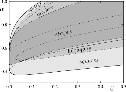
Figure 8: For $\eta=0.6$ and $g=0.5$ the parameter ranges are shown where stripes (dark), hexagon (medium) and squares (bright) have the lowest value for the functional ${\mathcal{F}}$. Along the dotted line one has ${\mathcal{F}}_{H}={\mathcal{F}}_{Q}$, along the dashed line ${\mathcal{F}}_{H}={\mathcal{F}}_{S}$, and along the dash-dotted line ${\mathcal{F}}_{S}={\mathcal{F}}_{Q}$.

Inserting the solutions of stripes in Eq. (40) and squares in Eq. (53) into their functionals in Eq. (39) and Eq. (51) the functionals can be reduced to very simple expressions

$${\mathcal{F}}_{S}=-\frac{1}{2\gamma}\eta^{2},\quad{\mathcal{F}}_{Q}=-\frac{1}{\gamma+\chi}\eta^{2}\,.$$ (67)

Hence the comparison of the functionals for squares and stripes is independent of the reduced control parameter $\eta$:

$${\mathcal{F}}_{Q}>{\mathcal{F}}_{S}\quad\Leftrightarrow\quad\chi>\gamma>0\,.$$ (68)

Accordingly the curves, cf. the dash-dotted line in Fig. 8, as calculated from the condition $\gamma=\chi$ of equal functional values, separate the regions where the functionals of stripes or squares have the lower values.

However, a comparison with the functionals for regular and inverse hexagons is not independent of $\eta$. Since hexagons bifurcate subcritically their amplitude is already finite and they have lower functional values at threshold $\eta=0$, i.e. ${\mathcal{F}}_{H}(\eta=0)<{\mathcal{F}}_{S}={\mathcal{F}}_{Q}=0$. Hexagons are therefore always preferred close to the threshold. Stripes and squares are always favored with respect to hexagons beyond some critical values $\eta>\eta_{S}(\alpha,\beta)$ and $\eta>\eta_{Q}(\alpha,\beta)$ which are determined by the conditions ${\mathcal{F}}_{H}={\mathcal{F}}_{S}$ and ${\mathcal{F}}_{H}={\mathcal{F}}_{Q}$, respectively. Accordingly, with decreasing values of $\eta$ the range in the $\alpha-\beta$ plane increases where hexagons have the lowest functional. As indicated by Fig. 9 the ranges of stripes and squares become smaller and smaller. For small values of $\eta$ square patterns are suppressed nearly completely.

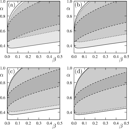
Figure 9: Dependence of the phase diagram of square, hexagon and stripe solutions (bright, medium and dark gray) on the control parameter $\eta$: (a)-(d) $\eta=0.6,0.4,0.2,0.1$, $g=0.5$. For small values of $\eta$ the region for hexagon solutions in the $\alpha$-$\beta$-plane increases and other solutions, squares quite more than stripe patterns, are suppressed.

For the interesting limiting case, $\alpha=1/2$ and $\beta\to 0$, one has $\delta=0$ and $\rho=6g+1/2$. Thus one expects in two spatial dimensions for $\beta\ll 1$ and $\alpha=1/2$ as well as small values of $\eta$ a clustering of ion channels to stripes. For finite values of $\beta$ and $\eta>0$ stripes are preferred to hexagons in the neighborhood of the curve $\delta=0$, cf. Fig. 6. This region broadens with increasing values of $\eta$, as indicated by Fig. 9.

IV.2.2 Linear stability analysis

A comparison of the values of the functionals for the respective patterns is one criterion for their basin of attraction. A linear stability analysis of the patterns shows, as described subsequently, that two patterns can both coexist in a region around the parameter range where their functionals agree.

Stripes vs. hexagons.

Stripes are still linearly stable even if their free energy is already higher than that of the hexagons, as can be seen by investigating the linear stability of stripes with respect to small amplitude perturbations $\delta A_{i}$

$$A_{1}=\sqrt{\frac{\eta}{\gamma}}+\delta\!A_{1},\qquad A_{2}=\delta\!A_{2},\qquad A_{3}=\delta\!A_{3}\,.$$ (69)

Linearizing Eqs. (60) with respect to the small functions $\delta\!A_{i}(t)$ and solving the resulting linear differential equations, one obtains the stability boundary as described by the condition (see e.g. Ref. Ciliberto:90.1 )

$$\eta\left(\gamma-\rho\right)^{2}-\gamma\delta^{2}>0\,.$$ (70)

By a similar stability analysis of the hexagonal solutions one obtains the following stability boundary Ciliberto:90.1

$$\eta\left(\gamma-\rho\right)^{2}-\left(\gamma-2\rho\right)\delta^{2}<0\,.$$ (71)

While stripes have the lower free energy between the solid lines in Fig. 8, stripes become only unstable at the dashed line and the hexagons at the dash–dotted line in Fig. 8.

Stripes vs. squares.

By a linear stability analysis of the stationary solutions given by Eq. (52) and by Eq. (53) one finds that stable stripes are preferred in the range $\chi>\gamma>0$ of the nonlinear coefficients and squares in the parameter range $|\chi|<\gamma$ Segel:65.1 . These ranges coincide with the ranges where both patterns have their lower functional values (cf. Eqs. (68)). Therefore stripe and square patterns do not coexist.

Squares vs. hexagons.

Numerical results in Sec. V.2 show that the amplitude equation for squares is a good approximation only for very small values of $\eta$. In this range square patterns are nearly completely suppressed by hexagonal pattern. Thus the quite complicated stability analysis of square patterns vs. hexagons (see e.g. Kubstrup:96.1 ) has been left out.

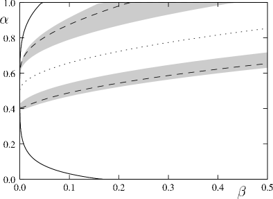
Figure 10: Range of coexistence of hexagons and stripes for $\eta=0.1$ and $g=0.5$. In the grey regions hexagons and stripes are both linearly stable with respect to small amplitude perturbations. Therefore both patterns coexist in a finite range around the dashed lines where their functionals agree, ${\mathcal{F}}_{S}={\mathcal{F}}_{H}$. Along the dotted line the nonlinear coefficient $\delta(\alpha,\beta)=0$ vanishes. The solid line indicates the region where both structures are limited by a cubic nonlinearity in their amplitude equations ($\gamma>0$ and $\gamma+2\rho>0$).

IV.3 “Nearly conserved case” - $\beta\propto\eta^{2}$

The amplitude equations for stripes, squares and hexagons were derived in Sec. IV.1 under the assumption of a finite wave number $k_{c}=\beta^{1/4}\propto O(1)$ and $k_{c}^{2}\gg\eta$. In the limit of a conserved number of open ion channels, i.e. $\beta=0$, beyond the onset of patter formation a clustering of channels takes place Fromherz:1989.1 , that may be described with a single component Cahn-Hilliard equation. In this section we show that in the limit of small values of the rate parameter $\beta$ with $\beta\propto\eta^{2}$ a reduction of Eqs. (13) to a single equation is still possible, whereby the resulting equation covers the qualitative properties of demixing as well as of periodic pattern formation.

From the previous section it is known that in the limit $\beta\to 0$ the bifurcation is subcritical in the range of small values of $\beta$, besides $\alpha=1/2$. Therefore the appropriate expansion, which leads also to finite amplitude solutions, is the combined expansion of $\beta\propto\eta^{2}$ and of $\alpha=1/2+\bar{\alpha}\sqrt{\eta}$ (with $\bar{\alpha}\propto O(1)$), as described in this section.

Expansion in the regime $\beta\propto\eta^{2}$ and $\alpha$ arbitrary.

In this case we expand the two fields $N$ and $V$ with respect to powers of $\eta$ in the following manner

$$N= \eta N_{0}+\eta^{2}N_{1}+\ldots\,\,\,,$$ (72a)

$$V= \eta V_{0}+\eta^{2}V_{1}+\ldots\,\,\,.$$ (72b)

In addition we also introduce slow space variables, $X,Y=\sqrt{\eta}\,x,\sqrt{\eta}\,y$, and a slow time variable $T=\eta^{2}t$. Choosing $\beta=\eta^{2}\tilde{\beta}$, with $\tilde{\beta}\propto O(1)$ and expanding Eqs. (13) with respect to powers of $\eta$ one obtains a single order parameter equation for $N_{0}$:

$$\partial_{T}N_{0}= -\tilde{\nabla}^{2}\left[\left(\tilde{\nabla}^{2}+1+2\sqrt{\tilde{\beta}}\right)N_{0}-\left(\alpha-\frac{1}{2}\right)N_{0}^{2}\right]$$

$$-\tilde{\beta}N_{0}$$ (73)

wherein $\tilde{\nabla}=(\partial_{X},\partial_{Y})$ has been used. The voltage follows immediately via the identity

$$V_{0}= -N_{0}\,.$$ (74)

By rescaling space, time as well as the amplitude ($\tilde{N}=\eta N_{0}$) this equation takes the form

$$\partial_{t}\tilde{N}= -\left(\nabla^{2}+\eta+2\sqrt{\beta}\right)\nabla^{2}\tilde{N},+\left(\alpha-\frac{1}{2}\right)\nabla^{2}(\tilde{N}^{2})$$

$$-\beta\tilde{N}\,,$$ (75a)

$$\tilde{V}= -\tilde{N}\,.$$ (75b)

This equation for $\tilde{N}$ shares similarities with the damped Kuramoto-Sivashinsky equation Kuramoto:84 ; CrossHo . The only difference is in the nonlinearity $\nabla^{2}(\tilde{N}^{2})=2((\nabla\tilde{N})^{2}+\tilde{N}\nabla^{2}\tilde{N})$ because the Kuramoto-Sivashinsky equation includes as nonlinearity $(\nabla\tilde{N})^{2}$ only. The additional term, $\tilde{N}\nabla^{2}\tilde{N}$, however, changes the dynamics and stability of the solutions completely beyond threshold, $\eta>0$. While one has for the Kuramoto-Sivashinsky equation “turbulent” but bounded solutions, the solutions of Eq. (75) are always divergent according to the nonlinear diffusion $\tilde{N}\nabla^{2}\tilde{N}$. For $\alpha=1/2$ the nonlinear coefficient in Eq. (75) vanishes completely, which suggests a different expansion close to this point, as described in the next paragraph.

Expansion in the regime $\beta\propto\eta^{2}$ and $\left(\alpha-\frac{1}{2}\right)\propto\sqrt{\eta}$.

Here also the parameter $\alpha$ is expanded with respect to the small parameter $\eta$: $\alpha=1/2+\sqrt{\eta\,}\tilde{\alpha}$ with $\tilde{\alpha}\propto O(1)$. Expanding the fields $N$ and $V$ with respect to powers of $\sqrt{\eta}$

$$N= \,\eta^{\frac{1}{2}}N_{0}+\eta N_{1}+\eta^{\frac{3}{2}}N_{2}+\dots\,,$$ (76a)

$$V= \,\eta^{\frac{1}{2}}V_{0}+\eta V_{1}+\eta^{\frac{3}{2}}V_{2}+\dots$$ (76b)

yields from Eq. (13) at leading order a single equation for $N_{0}$, which after rescaling $\tilde{N}=\sqrt{\eta\,}N_{0}$ takes the form

$$\partial_{t}\tilde{N}= -\nabla^{2}\left[\left(\nabla^{2}+\eta+2\sqrt{\beta}\right)\tilde{N}-\left(\alpha-\frac{1}{2}\right)\tilde{N}^{2}\right.$$

$$\left.-\left(\frac{1}{12}+g\right)\tilde{N}^{3}\right]-\beta\tilde{N}\,,$$ (77a)

$$\tilde{V}= -\tilde{N}\,.$$ (77b)

The cubic nonlinearity now limits the amplitudes of the solutions to finite values, because $1/12+g$ is positive even in the limit $\beta\to 0$. For $\beta=0$ and $\alpha=1/2$, corresponding to $\tilde{\alpha}=0$, the transition to the inhomogeneous channel distribution is continuous while it is discontinuous for $\tilde{\alpha}\neq 0$ but remains bounded. In the limit of a conserved channel density $\tilde{N}$, i.e. $\beta=0$, equation (77) is of the Cahn-Hilliard type Cahn:58.1 ; Lubensky:95 .

Eq. (77) covers all qualitative features of the basic equations (13) in both cases, in the limit $\beta=0$ and for $\beta\not=0$. Therefore, similar as in the previous section one can also derive the amplitude equations for stripes, squares and hexagons by starting from the modified equation (77) instead of Eqs. (13). These derivations are much simpler for Eq. (77) but the results are now restricted to a range along the line $\alpha\sim 1/2$, close to the threshold and to small values of the rate parameter $\beta\propto\eta^{2}$. Thereby one obtains again the amplitude equation for stripes as given by Eq. (32), for squares as by Eq. (47) and for hexagons as by Eq. (60), but now with slightly modified expressions for the coefficients.

$$\tau_{0} =\frac{1}{\sqrt{\beta}}, \delta =1-2\alpha,$$

$$\gamma =\frac{1}{4}+3g, \rho =\chi=\frac{1}{2}+6g.$$ (78)

These expressions may also be recovered from the formulas given in Sec. IV.1 in the limit $\beta\to 0$ and $\alpha\to 1/2$.

V Numerical Results

The amplitude equations, as given for the present system in the previous sections, are exemplarily derived in the appendix by a perturbational calculation. However, the validity range of these equations and their solutions is a priori unknown. An estimation of this range can be provided by comparing the analytical solutions with numerical simulations of the basic equations (13), as done in this section.

V.1 Stripe patterns

In the range of supercritically bifurcating stripe patterns determined analytically in the previous section, the analytical and numerical solutions of Eqs. (13) are compared in Fig. 11 as a function of the control parameter $\eta$ for $\alpha=0.4,\,\beta=0.1,\,g=0.5$ and $\tau_{V}=0.1$. There is a fairly good agreement between the analytical and the numerical solutions up to about $\eta=0.1$. Since the stripe pattern is stationary it does not depend on the actual value of $\tau_{V}$ used in simulations.

Figure 11: The amplitude of a stripe pattern as determined by the amplitude equation (solid line) and by numerical solutions of Eq. (13) (circles) are compared as a function of the control parameter. For the parameters $\alpha=0.4,~{}\beta=0.1,~{}g=0.5$ and $\tau_{V}=0.1$ the bifurcation was supercritical, i.e. $\gamma>0$.

V.2 Square patterns

Numerical simulations do not show stable square patterns besides transients to finally hexagonal patterns. Choosing a special geometry with a very small system length ($L=2\pi/k_{c}$) hexagonal patterns can be suppressed in numerical simulations. In this case the system shows the square patterns as predicted. By comparing the amplitudes $A_{i}$ as given for squares by Eq. (53) for $\alpha=0.4$, $\beta=0.1$ and $g=0.5$ with the numerical obtained solution, as depicted in Fig. 12, we find as a function of the reduced control parameter only an acceptable agreement for very small values of $\eta\lesssim 10^{-4}$. But then we find that squares are only preferred according to the analytical calculation in the range $\eta\gtrsim 0.1$, which is far beyond the validity range of the amplitude equations for squares. This is an explanation why we do not find the predicted squares by numerical solution of Eqs. (13).

Figure 12: The amplitudes of squares, $A_{1}=A_{2}$, are shown as a function of the reduced control parameter $\eta$ and for the parameters $\alpha=0.4$, $\beta=0.1$, $g=0.5$. The solid line is given by Eq. (53) and the circles are obtained from numerical simulations of the model equations.

V.3 Hexagonal patterns

Close to threshold hexagons are the preferred pattern in a wide range of parameters. In a range where stripes and squares bifurcate supercritically, but where hexagons are already preferred, at $\alpha=0.4$, $\beta=0.1$ and $g=0.5$, the analytically, cf. Eq. (66), and the numerically obtained solutions are compared in Fig. 13.

Figure 13: The amplitudes $A_{j}$ of the hexagonal pattern are given as a function of the reduced control parameter $\eta$. The solid line corresponds to the analytical solution $A_{+}$ and the dashed line belongs to the unstable solution $A_{-}$, where both are given by Eq. (66). The data points are obtained from the numerical solution of Eqs. (13). The parameters $\beta=0.1$, $\alpha=0.4$ and $g=0.5$ have been used.

V.4 Anharmonic solutions and clustering of ion channels for near conservation

Increasing the control parameter up to $\eta=0.9$, far beyond the validity range of the amplitude equations, the density $N(x)$ becomes rather anharmonic as shown in Fig. 14(b). Closer to the threshold at $\eta=0.04$ but in the range where stripes bifurcate subcritically and where the amplitudes take immediately large values, at $\alpha=0.95$ and $\alpha=0.03$, the solutions are also very anharmonic as shown for $N(x)$ in Fig. 14(a) and 14(c). In both cases each peak in Fig. 14(a) and (c) takes already a similar shape that are typical for the clusters in the conserved limit $\beta=0$.

Figure 14: The stationary and normalized distribution of ion channels $N(x)$ is shown for a stripe pattern above threshold for four different sets of parameters. In all cases $\beta=0.03$ and $g=0.1$ were fixed and therefore also the critical wave number $k_{c}=0.416$. The system length is $L=8\pi/k_{c}$.

VI Discussion and Conclusion

In Ref. Zimmermann:95.2 a model for the dynamics of ion channels including electrophoresis, an opening-closing reaction as well as a simultaneous binding-release reaction has been introduced. Compared to this earlier work, we have taken into account the effect of the excluded volume interaction between ion channel molecules. In addition the analysis of the bifurcations beyond the threshold of pattern formation has been extended to two spatial dimensions.

In terms of amplitude equations we give a detailed analysis of the competition between stripes, squares and hexagonal patterns. We have found that immediately above threshold hexagonal patterns are preferred in a large range of parameters, whereas further beyond the threshold stripes are preferred in an increasingly larger parameter range.

The validity range of the amplitude expansion has been tested by solving the model equations numerically with a pseudo-spectral code. By this comparison we have shown that the amplitude equations for squares have a very small validity range. The expansion for squares breaks down two orders of magnitude earlier than the one for stripes and hexagonal structures. Accordingly, the large range where square patterns should be favored as predicted by the amplitude expansion is not confirmed by the numerical analysis of the model equations while the amplitude equations describing the competition between stripes and hexagons are in a fairly good agreement with the numerical simulations close to the threshold.

In the limiting case $\beta\rightarrow 0$ implying a conserved number of open ion channels the patterns have a strong similarity with those patterns occurring during ion channel clustering Fromherz:1989.1 in systems with a binding-release reaction. Near threshold and in the limit of $\beta\propto\eta^{2}$ the model equations can be reduced to a single model equation which shares similarities with different variants of the Swift-Hohenberg equation CrossHo as well as the Cahn-Hilliard equation Cahn:58.1 ; Lubensky:95 . On the basis of this reduced equation essential effects related to the binding release reaction are already captured.

It is an interesting question whether the curvature of membranes influences the pattern competition especially between stripes and hexagons. One expects that in such a system the effects of a broken up-down symmetry become stronger leading to an additional enlargement of the parameter range where hexagonal patterns occur.

If the binding-release reaction is replaced by an opening-closing reaction, the formation of spatially periodic either stationary or oscillatory patterns has been reported SKramer:2002.1 ; RPeter:2006.100 . There the nonlinear behavior of stripe patterns has been discussed only partially and only in one spatial dimension. A competition of patterns as described in the present work will be expected but also a competition between two-dimensional stationary and time-dependent patterns.

Our calculations are related to experiments of the type as investigated in Ref. Rentschler:1998a where ion channels are studied in vitro. The electro-diffusive model at hand seems to be relevant for in vivo systems as shown by experiments on the effect of electric fields on clustering of acetylcholine receptors Leonetti:2005.1 ; Stollberg:88.1 ; Nitkin:90.1 . In membranes composed of several types of lipids a selforganized structuring has also been described in terms of lipid rafts Simons:1997a . Therefore one expects in such cases a spatially varying mobility of proteins embedded in the membrane. How this heterogeneity affects the formation of patterns is another interesting question as has been investigated for other model systems Zimmermann:1993a ; Schmitz:1996a ; Epstein:2001.2 ; Peter:2005a ; Hammele:2006.1 . A detailed analysis of all these questions may be given in forthcoming works.

Appendix A Derivation of the amplitude equation for the stripe pattern.

A.1 Basic equations in Matrix-Notation

Rewriting the basic Eqs. (13) to a matrix notation

$$({\mathcal{M}}\cdot\partial_{t}+{\mathcal{L}}){\bf u}={\bf N}({\bf u})\,,$$ (79)

allows a more compact formulation of the derivation of the generic amplitude equations of stripe patterns as given by Eq. (32), of square patterns as given by Eqs. (47) or of hexagonal patterns as given by Eqs. (60). The two components of the vector ${\bf u}$ are the normalized channel density $N$ and the reduced voltage $V$, whereas the matrices ${\mathcal{M}}$ and ${\mathcal{L}}$ represent the linear parts of Eqs. (13)

$${\mathcal{M}} =\left(\begin{array}[]{ccc}1&0\\ 0&0\\ \end{array}\right)\,, {\mathcal{L}} =\left(\begin{array}[]{ccc}\beta-\nabla^{2}\,\,\,\,,&-\nabla^{2}\\ \alpha(1-\alpha)\varepsilon\,,&1-\nabla^{2}\end{array}\right)\,,$$ (84)

and the vector ${\bf N}$ the nonlinearity:

$${\bf N} =\left(\begin{array}[]{c}\nabla\left(N\nabla V\right)+g\nabla^{2}(N^{3})\\ -\alpha NV\end{array}\right)\,.$$ (87)

The linear coefficients of Eq. (32) follow directly from the linear stability analysis as described in Sec. III and Sec. IV.1.1, but the nonlinear coefficient $\gamma$ in the same equation is determined by the perturbation expansion described in the next subsection.

A.2 Nonlinear coefficient

The sign of the nonlinear coefficient $\gamma$ in Eq. (32) determines, whether one has a sub- or a supercritical bifurcation to the periodic state given by Eq. (25). The scheme of the derivation of $\gamma$ and the respective amplitude equations may be found in various references, as for instance in Refs. CrossHo ; Newell:92.1 ; Zimmermann:93.1 . This scheme for the derivation of $\gamma$ is summarized for the present system in this appendix. The starting point is an expansion of the solutions of Eqs. (79) with respect to powers of the reduced control parameter $\eta$ as given by Eq. (24):

$${\bf u}({\bf r},t)=\eta^{\frac{1}{2}}{\bf u}_{0}({\bf r},t)+\eta\,{\bf u}_{1}({\bf r},t)+\eta^{\frac{3}{2}}{\bf u}_{2}({\bf r},t)+\dots\,.$$ (88)

Since the vector ${\bf N}$ is a nonlinear function of ${\bf u}$, it may be also expanded with respect to powers of $\eta$:

$${\bf N}({\bf u})=\eta\,{\bf N}_{1}({\bf u}_{0})+\eta^{\frac{3}{2}}\,{\bf N}_{2}({\bf u}_{0},{\bf u}_{1})+\ldots\enspace.$$ (89)

To the ansatz in Eq. (25) for a homogeneous stripe pattern

$${\bf u}_{0}={\bf\hat{e}}_{0}\,A\,e^{i{\bf k}_{c}{\bf r}}+c.c.$$ (90)

a multiscale analysis in time is added

$$\partial_{t}\rightarrow\partial_{t}+\eta\,\partial_{T}$$ (91)

to account for the variation of the amplitude $A=A(T)$ on a very slow time scale $T=\eta\,t$. Together with the relation $\varepsilon=\varepsilon_{c}(1+\eta)$ finally the basic equations in (79) may be rearranged into a powers series with respect to $\eta^{\frac{1}{2}}$ leading to the following hierarchy of equations:

$$\eta^{\frac{1}{2}} : \left({\mathcal{M}}\partial_{t}+{\mathcal{L}}_{0}\right){\bf u}_{0} =0\,,$$ (92)

$$\eta : \left({\mathcal{M}}\partial_{t}+{\mathcal{L}}_{0}\right){\bf u}_{1} ={\bf N}_{1}({\bf u}_{0})\,,$$ (93)

$$\eta^{\frac{3}{2}} : \left({\mathcal{M}}\partial_{t}+{\mathcal{L}}_{0}\right){\bf u}_{2} =-\left({\mathcal{L}}_{2}+{\mathcal{M}}\partial_{T}\right){\bf u}_{0}+{\bf N}_{2}({\bf u}_{0},{\bf u}_{1})$$ (94)

with the linear operators

$${\mathcal{L}}_{0} =\left(\begin{array}[]{ccc}\beta-\nabla^{2}\,\,\,\,,&-\nabla^{2}\\ \alpha(1-\alpha)\varepsilon_{c}\,,&1-\nabla^{2}\end{array}\right)\,,$$ (97)

$${\mathcal{L}}_{2} =\left(\begin{array}[]{ccc}0&0\\ \alpha(1-\alpha)\varepsilon_{c}&0\end{array}\right)$$ (100)

and the nonlinearities

$${\bf N}_{1} =\left(\begin{array}[]{c}\nabla\left(N_{0}\nabla V_{0}\right)\\ -\alpha N_{0}V_{0}\end{array}\right)\,,$$ (103)

$${\bf N}_{2} =\left(\begin{array}[]{c}\nabla(N_{0}\nabla V_{1}+N_{1}\nabla V_{0})+g\nabla^{2}N_{0}^{3}\\ -\alpha(N_{0}V_{1}+N_{1}V_{0})\end{array}\right).$$ (106)

Using the ansatz of Eq. (90) the leading contribution ${\bf N}_{1}({\bf u}_{0})$ of ${\bf N}({\bf u})$ has the explicit form

$${\bf N}_{1} =-E_{0}\left(\begin{array}[]{c}2k_{c}^{2}\,A^{2}e^{2i{\bf k}_{c}{\bf r}}\\ \alpha\left(A^{2}e^{2i{\bf k}_{c}{\bf r}}+|A|^{2}\right)\end{array}\right)+c.c.\,.$$ (109)

The solution ${\bf u}_{1}$ of Eq. (93) has to be of the same form as the inhomogeneity ${\bf N}_{1}$. This leads to the ansatz

$${\bf u}_{1}= \left(B_{1}{\bf\hat{e}}_{0}+B_{2}{\bf\hat{e}}_{1}\right)A^{2}e^{2i{\bf k}_{c}{\bf r}}+\left(B_{3}{\bf\hat{e}}_{0}+B_{4}{\bf\hat{e}}_{1}\right)|A|^{2}+c.c.$$ (110)

using the two eigenvectors ${\bf\hat{e}}_{0,1}=\left(1,E_{0,1}\right)$ of ${\mathcal{L}}_{0}$ with

$$E_{0} =-\left(1+\sqrt{\beta}\right)\,, E_{1} =\frac{1+\sqrt{\beta}}{\sqrt{\beta}}\,.$$ (111)

After inserting of (110) in (93) one obtains by comparison of coefficients:

$$B_{1} =\frac{1}{9}\left(10-\alpha+2\sqrt{\beta}+\frac{3\alpha}{\sqrt{\beta}(1+\sqrt{\beta})}+\frac{2-7\alpha}{\sqrt{\beta}}\right)\,,$$

$$B_{2} =\frac{1}{3}\left(2\sqrt{\beta}-\frac{\alpha\sqrt{\beta}}{1+\sqrt{\beta}}\right)\,,$$

$$B_{3} =-\frac{\alpha\sqrt{\beta}}{1+\sqrt{\beta}}\,,\hskip 28.45274ptB_{4}=-B_{3}\,.$$ (112)

At the next higher order, Eq. (94), one has to deal with the second order correction of the linear operator, ${\mathcal{L}}_{2}$, and of the vector ${\bf N}_{2}$ as defined in Eq. (100) and Eq. (106). It is not necessary to solve Eq. (94) explicitly. One can use Fredholm’s alternative or one simply can take advantage of the following property

$$\langle{\bf\hat{f}}_{0}e^{i{\bf k}_{c}{\bf r}},{\mathcal{L}}_{0}{\bf u}_{2}\rangle=\frac{1}{S}\int_{S}d{\bf r}~{}e^{-i{\bf k}_{c}{\bf r}}{\bf\hat{f}}_{0}^{\dagger}{\mathcal{L}}_{0}{\bf u}_{2}({\bf r},t)=0\,$$

of the left eigenvector

$${\bf\hat{f}}_{0}=\left(\begin{array}[]{c}1\\ F_{0}^{\star}\end{array}\right),\quad F_{0}=-\frac{\sqrt{\beta}}{1+\sqrt{\beta}},$$ (116)

which spans the adjoint kernel of ${\mathcal{L}}_{0}$. Since ${\bf u}_{0}$ and ${\bf u}_{1}$ have an explicit dependency only on the time scale $T$ but not on $t$ the corresponding derivatives can be neglected. Accordingly all the terms at the right hand side of Eq. (94) projected onto ${\bf\hat{f}}_{0}e^{i{\bf k}_{c}{\bf r}}$ also have to vanish:

$$\langle{\bf\hat{f}}_{0}e^{i{\bf k}_{c}{\bf r}},{\bf N}_{2}-\left({\mathcal{L}}_{2}+{\mathcal{M}}\partial_{T}\right){\bf u}_{0}\rangle=0\,.$$ (117)

This provides the solubility condition for the determination of the amplitude $A$. For this purpose the contributions to the expressions ${\mathcal{L}}_{2}{\bf u}_{0}$ and ${\bf N}_{2}$ which are proportional to $e^{i{\bf k}_{c}{\bf r}}$ are collected. According to the Fredholm’s alternative we obtain after projection

$$\gamma|A|^{2}A-A+\tau\partial_{T}A=0$$ (118)

with the nonlinear coefficient

$$\gamma = \frac{3g}{1+\sqrt{\beta}}-\frac{1}{3}\Big{[}\,\frac{6\alpha^{2}-\bigl{(}\alpha-2(1+\sqrt{\beta})\bigr{)}^{2}}{1+\sqrt{\beta}}$$ (119)

$$+\frac{2}{3\sqrt{\beta}}\bigl{(}4\sqrt{\beta}-2\alpha+1\bigr{)}\bigl{(}\sqrt{\beta}-2\alpha+1\bigr{)}\,\Big{]}\,,$$

and the relaxation time

$$\tau=\frac{1}{\sqrt{\beta}\left(1+\sqrt{\beta}\right)}\,.$$ (120)

The nonlinear coefficient depends on the rate parameter $\beta$, the density parameter $\alpha$ and on the parameter $g$ for the excluded volume interaction. The relaxation time of the pattern as well as the nonlinear coefficient $\gamma$ both diverge for a frozen binding-release reaction ($\beta\rightarrow 0$). In this limit the wave number $k_{c}$ tends to zero and the assumptions made for the derivation of the amplitude equation are not longer fulfilled.

References

- (1) M. C. Cross and P. C. Hohenberg, Rev. Mod. Phys. 65, 851 (1993).
- (2) Spatio-Temporal Patterns in Nonequilibrium Complex Systems, Vol. XXI of Santa Fe Institute Studies in the Sciences of Complexity, edited by P. Cladis and P. Palffy-Muhoray (Addision-Wesley, New York, 1995).
- (3) P. Manneville, Dissipative Structures and Weak Turbulence (Academic Press, London, 1990).
- (4) J. D. Murray, Mathematical Biology (Springer, Berlin, 1989).
- (5) F. Nédélec et. al., Nature 389, 305 (1997).
- (6) H. Y. Lee and M. Kardar, Phys. Rev. E 64, 056113 (2001).
- (7) T. B. Liverpool and M. C. Marchetti, Phys. Rev. Lett. 90, 138102 (2003).
- (8) F. Ziebert and W. Zimmermann, Eur. Phys. J E 18, 41 (2005).
- (9) F. Ziebert and W. Zimmermann, Phys. Rev. E 70, 022902 (2004).
- (10) A. V. Panfilov and P. Horteweg, Science 270, 1223 (1995).
- (11) S. Kondo and R. Asai, Nature (London) 376, 765 (1995).
- (12) E. Mandelkow et al., Science 246, 1291 (1989).
- (13) H. Oberman, E. M. Mandelkow, G. Lange, and E. Mandelkow, J. Bio. Chem. 265, 4382 (1990).
- (14) M. Hammele and W. Zimmermann, Phys. Rev. E 67, 021903 (2003).
- (15) K. Kruse and F. Jülicher, Curr. Op. Cell Bio. 17, 20 (2005).
- (16) S. J. Singer and G. L. Nicolson, Science 175, 720 (1972).
- (17) P. Fromherz, Proc. Natl. Acad. Sci. USA 85, 6353 (1988).
- (18) P. Fromherz, Ber. Bunsenges. Phys. Chem. 92, 1010 (1988).
- (19) P. Fromherz and B. Kaiser, Europhys. Lett. 15, 313 (1991).
- (20) P. Fromherz and A. Zeiler, Physics Lett. A 190, 33 (1994).
- (21) P. Fromherz and W. Zimmermann, Phys. Rev. E 51, R1659 (1995).
- (22) S. C. Kramer and R. Kree, Phys. Rev. E 65, 051920 (2002).
- (23) M. Leonetti, P. Marcq, J. Nuebler, and F. Homble, Phys. Rev. Lett. 95, 208105 (2005).
- (24) R. Peter and W. Zimmermann, Phys. Rev. E 74, 016206 (2006).
- (25) E. Neher and B. Sakmann, Nature (London) 260, 799 (1976).
- (26) L. F. Jaffe, Nature (London) 265, 600 (1977).
- (27) J. Stollberg and S. E. Fraser, J. Cell Biol. 107, 1397 (1988).
- (28) R. M. Nitkin and T. C. Rothschild, J. Cell Biol. 111, 1161 (1990).
- (29) H. B. Peng and M. Poo, Trends Neurosci. 9, 125 (1986).
- (30) K. Simons and E. Ikonen, Nature 387, 569 (1997).
- (31) D. J. Aidley and P. R. Stanfield, Ion Channels (Cambridge Univ. Press, Cambridge, 1996).
- (32) F. Guharay and F. Sachs, J. Physiol. (London) 352, 685 (1984).
- (33) L. P. Savchenko, S. N. Antropov, and S. M. Korogod, Biophys. J. 78, 1119 (2000).
- (34) P. Fromherz and B. Klingler, Biochim. Biophys. Acta 1062, 103 (1991).
- (35) L. P. Savchenko and S. M. Korogod, Neurophysiology 26, 78 (1994).
- (36) M. Leonetti, Euro. Phys. J. B 2, 325 (1998).
- (37) A. C. Scott, Rev. Mod. Phys. 47, 487 (1975).
- (38) J. J. B. Jack, D. Noble, and R. W. Tsien, Electric current flow in excitable cells (Clarendon Press, Oxford, 1975).
- (39) B. Hille, Ionic Channels of Excitable Membranes (Sinauer, Sunderland, 1992).
- (40) A. C. Newell, T. Passot, and J. Lega, Annu. Rev. Fluid Mech. 25, 399 (1992).
- (41) W. Zimmermann, Mat. Res. Bulletin 16, 46 (1991).
- (42) H. R. Brand, P. Lomdahl, and A. C. Newell, Physica (Nonlin. Phenomena) D 23, 345 (1986).
- (43) W. Schöpf and W. Zimmermann, Phys. Rev. E 47, 1739 (1993).
- (44) S. Ciliberto et al., Phys. Rev. Lett. 65, 2370 (1990).
- (45) L. A. Segel, J. Fluid Mech. 21, 359 (1965).
- (46) C. Kubstrup, H. Herrero, and C. Pérez-Garcia, Phys. Rev. E 54, 1560 (1993).
- (47) P. Fromherz, Chem. Phys. Lett 154, 147 (1989).
- (48) Y. Kuramoto, Chemical Oscillations, Waves, and Turbulence (Springer, Berlin, 1984).
- (49) J. W. Cahn and J. E. Hilliard, J. Chem. Phys. 28, 258 (1958).
- (50) P. M. Chaikin and T. C. Lubensky, Principles of condensed matter physics (Cambridge Univ. Press, Cambridge, UK, 1995).
- (51) M. Rentschler and P. Fromherz, Langmuir 14, 547 (1998).
- (52) W. Zimmermann, M. Seesselberg, and F. Petruccione, Phys. Rev. E 48, 2699 (1993).
- (53) R. Schmitz and W. Zimmermann, Phys. Rev. E 53, 5993 (1996).
- (54) A. Sanz-Anchelergues, A. M. Zhabotinsky, I. R. Epstein, and A. P. Munuzuri, Phys. Rev. E 63, 056124 (2001).
- (55) R. Peter et al., Phys. Rev. E 71, 046212 (2005).
- (56) M. Hammele, S. Schuler and W. Zimmermann, Physica D (Nonlinear Science) 218, 139 (2006).