The Surface Topography of a Magnetic Fluid — 
a Quantitative Comparison between Experiment and Numerical Simulation

Abstract

The normal field instability in magnetic liquids is investigated experimentally by means of a radioscopic technique which allows a precise measurement of the surface topography. The dependence of the topography on the magnetic field is compared to results obtained by numerical simulations via the finite element method. Quantitative agreement has been found for the critical field of the instability, the scaling of the pattern amplitude and the detailed shape of the magnetic spikes. The fundamental Fourier mode approximates the shape to within $10\,\%$ accuracy for a range of up to $40\,\%$ of the bifurcation parameter of this subcritical bifurcation. The measured control parameter dependence of the wavenumber differs qualitatively from analytical predictions obtained by minimization of the free energy.

1 Introduction

Pattern formation has mostly been investigated in systems driven far from equilibrium, like Rayleigh–Bénard convection, Taylor–Couette flow (cf. Cross & Hohenberg, 1993) or current instabilities Peinke et al. (1992). This lopsided orientation is partly due to the belief that mainly systems far from equilibrium can bring us a step forward to comprise fundamental riddles like the origin of life on earth Prigogine (1988).

However, conservative systems may also exhibit the formation of patterns, a typical example being given by elastic shells under a buckling load Taylor (1933); Lange & Newell (1971). In particular, these non-dissipative systems have recently gained interest within the context of life: following Shipman & Newell (2004) they can describe pattern formation in plants. Closely related are surface instabilities of dielectric liquids in electric fields Taylor & McEwan (1965) and its magnetic counterpart, first observed by Cowley & Rosensweig (1967). In comparison with shell structures, the surface instabilities are experimentally more accessible because the external field can serve as a convenient control parameter.

In order to observe the Rosensweig, or normal field instability, a horizontally extended layer of magnetic fluid is placed in a magnetic field oriented normally to the flat fluid surface. When exceeding a critical value $B_{c}$ of the applied magnetic induction, one can observe a hysteretic transition between the flat surface and a hexagonal pattern of liquid crests. The transition gains some complexity from the fact that under variation of the surface three terms of the energy are varying, namely the hydrostatic energy (determined via the height variation of the liquid layer), the surface energy and the magnetic field energy. As the surface profile deviates from the flat reference state, the first two terms grow whereas the magnetic contribution decreases. At the critical field, the overall energy is minimized by a static surface pattern of finite amplitude.

Using the energy minimization principle, Gailitis (1969, 1977) and Kuznetsov & Spektor (1976) were able to deduce an amplitude equation that connects the instability to a subcritical bifurcation. However, this result is limited to tiny susceptibilities $\chi_{0}\ll 1$. Only recently this deficiency was partly overcome by Friedrichs & Engel (2001) for the normal field instability, and by Friedrichs (2002) for the more general case of the tilted field instability. Besides these achievements, the nonlinear stability of surface patterns under the assumption of a linear magnetization law was studied numerically by Boudouvis et al. (1987).

From an experimental point of view, the above predictions have been poorly investigated. This is mainly due to the experimental difficulties in measuring the surface profiles. Due to their colloidal nature, magnetic fluids are opaque and have a very poor reflectivity Rosensweig (1985). They appear black to the naked eye. Thus standard optical techniques such as holography or triangulation Perlin, Lin & Ting (1993) are not successful. Moreover, the fully developed crests are much too steep to be measured with optical shadowgraphy, as proposed by Browaeys et al. (1999), utilizing the slightly deformed surface as a (de)focusing mirror for a parallel beam of light. Another method, recently accomplished by Wernet et al. (2001), analyzes the reflections of a narrow laser beam in a Faraday experiment. However, it yields only the local surface slope, but not the local surface height. This has now been overcome by Megalios et al. (2005). By adapting the focus of a laser beam, a height detection is possible. However, the method has deficiencies in accuracy, because the beam partly penetrates the magnetic fluid. Moreover, it is limited to maxima and minima whereas measurements of the full surface topography are not possible.

A surface profile can be obtained by simple lateral observation of the instability, as implemented e.g.  by Mahr & Rehberg (1998a) for a single Rosensweig peak and by Bacri & Salin (1984) and Mahr & Rehberg (1998b) for a chain of peaks. It has, however, the severe disadvantage that the observed crests are next to the container edge. Therefore, they are deeply affected by the meniscus and field inhomogeneities. A comparison with the theory for an infinitely extended layer of magnetic fluid has remained unsatisfactory for a long time. Consequently, only the ‘flat aspects’ of the pattern like the wavenumber Abou, Wesfreid & Roux (2001); Lange, Reimann & Richter (2000); Reimann, Richter, Rehberg & Lange (2003) or the dispersion relation Mahr, Groisman & Rehberg (1996); Browaeys, Bacri, Flament, Neveu & Perzynski (1999) has been thoroughly investigated in experiments so far.

Recently we have developed a radioscopic measurement technique that utilizes the attenuation of an X-ray beam to measure the full three-dimensional surface profile of the magnetic fluid far away from the container edges Richter & Bläsing (2001).

The aim of this article is to compare thoroughly the measured surface profile of the instability with the analytical predictions and with novel numerical results obtained by Matthies & Tobiska (2005) via finite element methods.

The paper is organized as follows. In the next section we give a description of the experimental methods. Then the numerical methods of the corresponding simulations are explained. In the fourth section the experimental and numerical results are presented in parallel. Eventually, we compare and discuss these results.

2 Experimental methods

In the following, we give a description of the experimental setup, the necessary image corrections, and the calibration of the height profile. Finally we characterize the utilized magnetic liquid.

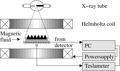
Figure 1: Setup of the radioscopic measurement of the surface topography

We measure the surface topography of the pattern via the attenuation of X-rays passing the magnetic fluid layer in vertical direction. Figure 1 shows the experimental setup. A container is placed in the centre of a Helmholtz pair of coils. The container is machined from Macrolon^® and has a diameter of $170\,$mm, and a depth of $25\,$mm. In order to minimize the field inhomogeneity at the container edge due to the discontinuity of the magnetization, we have introduced a ‘beach’. The floor of the container is flat within a diameter of $130\,$mm, outside of which it is inclined upwards at $32$ degrees, so that the thickness of the fluid layer smoothly decreases down to zero towards the side of the vessel. The container is filled $10\,$mm deep with magnetic fluid. This filling depth is in the range of the critical wavelength ($9.98\,$mm) which ensures according to Lange (2001) that finite size effects in vertical direction can be excluded.

The two Helmholtz coils have an inner bore of $29\,\mathrm{cm}$ (Oswald Magnettechnik) and a vertical separation distance of $18.5\,\mathrm{cm}$. The field homogeneity within the empty coils is better than $0.5\,\%$ within the volume covered by the vessel. The coils are supplied by a high precision constant current source (Heinzinger PTNhp 32-40) which allows to control the magnetic induction in steps of $1\,\mathrm{\math@atom{\mu}{\mathchoice{\hbox{$\displaystyle\mu$}}{\hbox{$\textstyle\mu$}}{\hbox{$\scriptstyle\mu$}}{\hbox{$\scriptscriptstyle\mu$}}}T}$ up to a maximum induction of $40\,\mathrm{mT}$.

An X-ray tube with a focus of $0.4\,\mathrm{mm}\times 1.2\,\mathrm{mm}$ is mounted above the centre of the vessel at a distance of $170\,\mathrm{cm}$. The tube has a wolfram anode in order to emit purely continuous radiation in the range of the applied acceleration voltage (20 kV to 60 kV). This ensures that the beam hardness can be adapted to the absorption coefficient of the fluid investigated. The radiation transmitted through the fluid layer and the bottom of the vessel is recorded by means of an X-ray sensitive photodiode array detector. The detector provides a dynamic range of 16 bits, a lateral resolution of $0.4\,\mathrm{mm}$, and a maximum frame rate of $7.5$ pictures per second. For more details see the article by Richter & Bläsing (2001).

2.1 Image improvement

Because of deficiencies of the X-ray detector, various digital filters had to be applied to improve the image quality.

First, there are so called ‘bad pixels’. These are non-functional sensors which must be ignored during image processing. The position of those bad pixels has been extracted from an empty test image by looking for all pixels the value of which deviates more than $10\,\%$ from the median of their neighbours. There are single isolated bad pixels as well as few unusable rows and columns. Correction is achieved by discarding the value of the bad pixels and filling the gap with a bilinear interpolation from the neighbourhood. This correction of bad pixels can be seen as the first approximation of the Voronoi-Allebach algorithm Sauer & Allebach (1987). It is a reasonable approach when the non-functional pixels do not form large clusters, but are rather scattered.

Second, the detector exhibits a nonlinear response, and individual pixels are not equally sensitive. Let $I$ denote the real incoming intensity and $r$ the response from the pixel, both normalized to the range $\left[0\dots 1\right]$. Then we fit the inverse response function of every individual pixel with a cubic polynomial

$$I(r)=a_{1}r^{3}+a_{2}r^{2}+a_{3}r+a_{4}.$$ (1)

The reference data for this model comes from $26$ empty test images with different illumination.

This method has an additional advantage of equalizing spatial inhomogeneities in the illumination caused by the nonuniformity of the intensity of the beam. This non-uniform illumination is contained in the image set used for the calibration. Thus we can safely assume that after the nonlinear correction the value of every pixel is directly proportional to the absorption of X-rays at the corresponding point. The assumption, however, is that the illumination itself does not change over time.

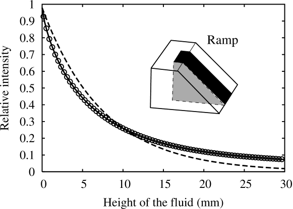
Figure 2: Fluid height versus radiation intensity. The inset shows a schematic view of the wedge filled with ferrofluid. The relative amount of the X-rays passing through the ramp can be fitted nicely with a sum of exponential functions (solid line, equation 3). A simple exponential decay with one attenuation coefficient is not sufficient (dashed line, equation 2).

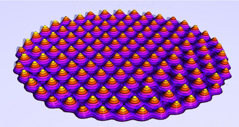
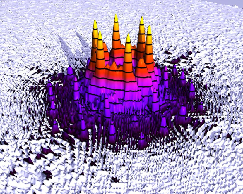
Figure 3: Three-dimensional rendering of the surface pattern at $B=20.1068\,$mT. The black contour lines are $1\,$mm apart from each other.

Figure 4: Logarithmic Fourier space representation of the surface in figure 4. The black contour lines are $6\,$dB apart from each other.

2.2 Conversion from intensity values to surface height profiles

The intensity of the X-rays decreases monotonically with the height of the fluid due to absorption. The slope of the surface has no influence on the transmitted intensity, since X-rays have indices of refraction very close to $1$.

If the radiation would be monochromatic, then the decay would follow an exponential law

$$I(x)=I_{0}\mathrm{e}^{-\beta x},$$ (2)

where $\beta$ is the attenuation coefficient. However, in order to get a sufficient illumination, we have to use a polychromatic X-ray source. Hence, the absorption of the radiation depends on the wavelength and the decay cannot be described by the simple exponential function (2): radiation of higher energy (‘hard X-rays’) is generally absorbed less than radiation of lower energy. In order to get a smooth approximation of the attenuation, we fit the intensity decay with an overlay of four exponential functions, as shown in figure 2.

$$I(x)=I_{0}\,\sum_{i=1}^{4}\alpha_{i}\mathrm{e}^{-\beta_{i}x},\quad\sum_{i=1}^{4}\alpha_{i}=1$$ (3)

The datapoints were obtained by recording the absorption image of a ramp with known shape filled with ferrofluid, see the inset in figure 2. To hold the ferrofluid in position, we covered the bottom and the side of the wedge with adhesive tape. The absorption in this tape lowers the effective intensity of the X-rays in the fluid by about $1\,\%$, which has been taken into account for the calculation of the absorption in the fluid.

As can be seen from figure 2, the equation (3) is a satisfactory interpolation method that allows us to determine the height of the fluid above every point in the image to a resolution of up to $10\,\mathrm{\math@atom{\mu}{\mathchoice{\hbox{$\displaystyle\mu$}}{\hbox{$\textstyle\mu$}}{\hbox{$\scriptstyle\mu$}}{\hbox{$\scriptscriptstyle\mu$}}}m}$. The absolute accuracy is not as good because of practical problems. For example, it is difficult to determine the exact position of the wedge either mechanically (because of its sharp end) or from the X-ray image due to the lateral resolution of $0.4\,$mm. This means that the absolute error of the fluid height will be around $\pm 0.2\,$mm. However, when measuring the pattern amplitude defined as a difference between the maximum and minimum surface elevation in the unit cell, this systematic error cancels.

After applying the corrections from the previous sections, we finally arrive at the surface profile. A three-dimensional reconstruction of one of the recorded profiles is shown in figure 4. The corresponding Fourier transform is displayed in figure 4. It should be noted that we get the Fourier space representation of the surface elevation using the radioscopic method, in contrast to other methods where the transform of a photograph is used. This allows for interpretation of the Fourier domain data as amplitudes which will be exploited later on in this paper.

2.3 Tracking one single peak

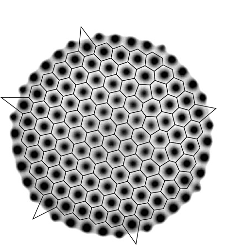
Figure 5: X-Ray image and Voronoi diagram constructed from the centre of the peaks

Both analytical and numerical predictions are based on the assumption that the pattern of peaks is periodic in space. But a perfect periodic lattice is not observed in this experiment. For example, one can see a grain boundary between two different orientations at the right side of the recorded profile in figure 4. Additionally, as mentioned in the introduction, peaks in the centre of the container are least affected by the edge. Thus, we select one single peak from there. Because the peak floats slightly under variation of the magnetic induction, it is further necessary to track it from image to image.

To accomplish this, we first determine the position of all peaks with subpixel accuracy by fitting a paraboloid to the centre of the peaks, and then construct the Voronoi tesselation from these positions. The region occupied by the considered peak is then defined by its Voronoi cell, i.e. every point in this region is closer to the considered peak centre than to any other peak Fortune (1995). We track the movement of the considered peak on two consecutive images by finding the Voronoi cell on the later image in which the previous position of the peak is situated. Figure 5 visualizes the tesselation. Note that the Voronoi diagram also exposes the grain boundary made up of a chain of penta-hepta defects.

The paraboloidal fit also yields the maximum level of this single peak. The minimum level in the hexagonal grid is reached at the corners of the unit cell. Therefore, their arithmetic mean value is taken as the minimum level. The amplitude of the pattern is then defined as the difference between the maximum and minimum level.

2.4 Properties of the magnetic liquid

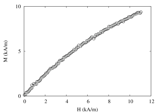
Figure 6: Magnetization curve of the ferrofluid APG512a from Ferrotec Co. The solid line is a fit with the Langevin equation (4).

We have selected the commercial magnetic fluid APG512a (Lot F083094CX) from Ferrotec Co. because of its convenient wavenumber and its outstanding long-term stability. The critical field of two data series that are $5$ months apart differs by not more than $1\,\%$. This can be attributed in part to its carrier liquid, a synthetic ester, which is commonly used as oil for vacuum pumps. The magnetic fluid is based on magnetite.

Quantity		Value $\pm$	Error
Surface tension	$\sigma$	$30.57\ \pm$	$0.1\,\mathrm{mN\,m^{-1}}$
Density	$\rho$	$1236\ \pm$	$5\,\mathrm{kg\,m^{-3}}$
Viscosity	$\eta$	$120\ \pm$	$5\,\mathrm{mPa\,s}$
Saturation magnetization	$M_{S}^{\ast}$	$14590\ \pm$	$100\,\mathrm{A\,m^{-1}}$
Initial susceptibility	$\chi_{0}$	$1.172\ \pm$	$0.005$

Table 1: Material parameters of the magnetic fluid.

The characteristic properties that have an influence on the normal field instability can be found in table 1. The density of the fluid has been measured using a buoyancy method and the surface tension coefficient has been determined using a commercial ring tensiometer.

The magnetization law $M(H)$ in the interesting range is shown in figure 6. Because the fluid is polydisperse, it cannot be expected that the magnetization law is a true Langevin function. However, fitting a Langevin function to the initial range of the magnetization curve leads to satisfactory results, as used before by Browaeys et al. (1999). The magnetization law reads therefore

$$\boldsymbol{M}(\boldsymbol{H})=M_{S}^{\ast}\left(\coth(\gamma|\boldsymbol{H}|)-\frac{1}{\gamma|\boldsymbol{H}|}\right)\frac{\boldsymbol{H}}{|\boldsymbol{H}|},\quad\gamma=\frac{3\chi_{0}}{M_{S}^{\ast}}.$$ (4)

This approximation is, of course, only valid in the initial range up to an internal field of about $H_{\text{int}}=12\,\mathrm{kA\,m^{-1}}$. The maximum internal field in the simulation is fully contained within this range.

The onset of the instability can be predicted from these material parameters by the linear stability analysis according to Rosensweig (1985), § 7.1. The critical magnetization $M_{c}$ of the fluid layer is given by

$$M_{c}^{2}=\frac{2}{\mu_{0}}\left(1+\frac{1}{r_{0}}\right)(g\rho\sigma)^{1/2},$$ (5a)

where

$$r_{0}=\sqrt{\mu_{c}\mu_{t}}/\mu_{0},\quad\mu_{c}=\frac{B}{H}\quad\text{and}\quad\mu_{t}=\frac{\math@atom{\partial}{\mathchoice{\hbox{$\displaystyle\partial$}}{\hbox{$\textstyle\partial$}}{\hbox{$\scriptstyle\partial$}}{\hbox{$\scriptscriptstyle\partial$}}}B}{\math@atom{\partial}{\mathchoice{\hbox{$\displaystyle\partial$}}{\hbox{$\textstyle\partial$}}{\hbox{$\scriptstyle\partial$}}{\hbox{$\scriptscriptstyle\partial$}}}H}.$$ (5b)

Together with $M(H)$ and the jump condition of the magnetic field at the ground of the dish,

$$B_{c}=H+M(H),$$ (6)

the critical induction can be determined from these implicit equations. For the values from table 1, we get $B_{c}=17.22\,\mathrm{mT}$.

The critical wavenumber $k_{c}$ from this analysis is given by

$$k_{c}=\sqrt{\frac{\rho g}{\sigma}}.$$ (7)

With our parameters, this yields $k_{c}=0.629\,\mathrm{mm^{-1}}$, which corresponds to a wavelength $\lambda_{c}=9.98\,\mathrm{mm}$.

3 Numerical methods

Our numerical simulation of the normal field instability is based on the coupled system of the Maxwell equations and the Navier–Stokes equations together with the Young–Laplace equation which represents the force balance at the unknown free interface. In this section we want to describe a numerical algorithm for the simulation of the coupled system of partial differential equations. Simplified numerical models have been studied already, see Boudouvis et al. (1987) and Lavrova et al. (2003). In this paper, we focus on the computation of the peak shapes employing a realistic magnetization curve in the form of the nonlinear Langevin function. This is in contrast to Boudouvis et al. (1987) where the stability of hexagonal and square pattern was considered for a linear magnetization law.

We consider a horizontally unbounded and infinitely deep layer of ferrofluid. The Maxwell equations for the non-conducting ferrofluid reduce to

$$\text{curl }\boldsymbol{H}=\boldsymbol{0},\qquad\text{div }\boldsymbol{B}=0.$$

The magnetization inside the fluid is assumed to follow equation (4) while there is no magnetization outside the fluid. The Navier–Stokes equations are given by

$$\rho\left(\frac{\math@atom{\partial}{\mathchoice{\hbox{$\displaystyle\partial$}}{\hbox{$\textstyle\partial$}}{\hbox{$\scriptstyle\partial$}}{\hbox{$\scriptscriptstyle\partial$}}}\boldsymbol{u}}{\math@atom{\partial}{\mathchoice{\hbox{$\displaystyle\partial$}}{\hbox{$\textstyle\partial$}}{\hbox{$\scriptstyle\partial$}}{\hbox{$\scriptscriptstyle\partial$}}}t}+(\boldsymbol{u}\cdot\boldsymbol{\nabla})\boldsymbol{u}\right)-\boldsymbol{\nabla}\cdot\boldsymbol{\tau} =-\rho g\boldsymbol{e}_{z},$$ (8)

$$\text{div }\boldsymbol{u} =0,$$ (9)

where $\boldsymbol{\tau}$ is the stress tensor given by

$$\boldsymbol{\tau}=\eta\left(\boldsymbol{\nabla}\boldsymbol{u}+\boldsymbol{\nabla}\boldsymbol{u}^{T}\right)-\left(p+\frac{\mu_{0}}{2}H^{2}\right)\mathsfbi{I}+\boldsymbol{H}\otimes\boldsymbol{B}.$$

Here, $\mathsfbi{I}$ denotes the unit tensor, $\otimes$ is the tensor product, and $p=p_{\text{hyd}}+p_{m}$ is the sum of the hydrostatic pressure $p_{\text{hyd}}$ and the fluid-magnetic pressure

$$p_{m}=\mu_{0}\int\limits_{0}^{H}M(h)\,\mathrm{d}h.$$

In the static case we are considering here ($\boldsymbol{u}\equiv\boldsymbol{0}$), the Navier–Stokes equations reduce to

$$\boldsymbol{\nabla}p=-\rho g\boldsymbol{e}_{z}+\mu_{0}M\boldsymbol{\nabla}H.$$ (10)

The Young–Laplace equation, which represents the force balance at the interface, reads as follows

$$[|\boldsymbol{\tau}|]\boldsymbol{n}=\sigma\mathcal{K}\boldsymbol{n},$$ (11)

where $\sigma$ is the coefficient of the surface tension, $\mathcal{K}$ the sum of the principal curvatures and $[|\boldsymbol{\tau}|]$ the jump of stress tensor.

Integrating the pressure equation (10) and inserting the Young–Laplace equation (11), we obtain the relation

$$\sigma\mathcal{K}+\rho gz=\mu_{0}\int\limits_{0}^{H}M(h)\,\mathrm{d}h+\frac{\mu_{0}}{2}(\boldsymbol{M}\boldsymbol{\cdot}\boldsymbol{n})^{2}-p_{0}.$$ (12)

Here the two terms on the left-hand side characterize the surface energy and the hydrostatic energy, while the first two terms on the right-hand side capture the energy due to the presence of a magnetic fluid. The pressure $p_{0}$ in (12) is a constant reference pressure.

For the numerical simulation we consider a bounded domain $\widetilde{\Omega}\times(\widetilde{z}_{b},\widetilde{z}_{t})$ which is chosen in a way that the hexagon $\widetilde{\Omega}$ contains exactly one peak. Furthermore, the boundaries in $\widetilde{z}$-direction are assumed to be far away from the interface. Now, the problem is transformed into its dimensionless form by using the strength of the applied field for all magnetic quantities and a characteristic length scale $l$ which is usually a fixed multiple of the wavelength. The domain obtained in this way will be denoted by $\Omega\times(z_{b},z_{t})$.

The Maxwell equations in dimensionless form read

$$\text{curl }\boldsymbol{H}=\boldsymbol{0},\quad\text{div }\boldsymbol{B}=0,\qquad\text{in }\Omega\times(z_{b},z_{t}).$$ (13)

The first differential equation in (13) ensures the existence of a scalar magnetostatic potential $\varphi$ so that $\boldsymbol{H}=-\boldsymbol{\nabla}\varphi$. Hence, by exploiting the second differential equation of (13), we get

$$-\text{div}\big{(}\mu(\boldsymbol{x},|\boldsymbol{\nabla}\varphi|)\boldsymbol{\nabla}\varphi\big{)}=0\qquad\text{in }\Omega\times(z_{b},z_{t}).$$ (14)

The coefficient function $\mu(\boldsymbol{x},H)$ is given by

$$\mu(\boldsymbol{x},H)=\begin{cases}1&\boldsymbol{x}\in\Omega_{A},\\ \displaystyle 1+\frac{M(H)}{H}&\boldsymbol{x}\in\Omega_{F},\end{cases}$$

where $\Omega_{F}$ and $\Omega_{A}$ are the subdomains of $\Omega\times(z_{b},z_{t})$ which correspond to the regions inside and outside the ferrofluid, respectively. The magnetostatic problem (14) is a nonlinear uniformly elliptic partial equation. The nonlinearity in (14) is resolved by a fixed-point iteration. The partial differential equation (14) is equipped with the following boundary conditions: $\varphi=-zH^{(F)}$ at the bottom boundary $z_{b}$, $\varphi=-zH^{(A)}$ at the top boundary $z_{t}$, and $\math@atom{\partial}{\mathchoice{\hbox{$\displaystyle\partial$}}{\hbox{$\textstyle\partial$}}{\hbox{$\scriptstyle\partial$}}{\hbox{$\scriptscriptstyle\partial$}}}\varphi/\math@atom{\partial}{\mathchoice{\hbox{$\displaystyle\partial$}}{\hbox{$\textstyle\partial$}}{\hbox{$\scriptstyle\partial$}}{\hbox{$\scriptscriptstyle\partial$}}}n=0$ at the side boundary. Here, $H^{(A)}$ and $H^{(F)}$ denote the constant strength of the magnetic field outside and inside the ferrofluid in the case of an undisturbed interface, respectively. Moreover, $H^{(F)}$ can be obtained from $H^{(A)}$ by a single algebraic equation.

In the consideration of the Young–Laplace equation we assume that the interface $\Gamma$ is the graph of a function $\Psi:\Omega\to\mathbb{R}$, i.e.,

$$\Gamma=\big{\{}(x,y,z)\in\mathbb{R}^{3}\>:\>z=\Psi(x,y),\>(x,y)\in\Omega\big{\}}.$$

Now, the sum of the principal curvatures can be written in terms of $\Psi$. We have

$$\mathcal{K}=-\text{div}\frac{\boldsymbol{\nabla}\Psi}{\sqrt{1+|\boldsymbol{\nabla}\Psi|^{2}}}.$$

Hence, after dividing by $\sigma$, the Young–Laplace equation is given by

$$-\text{div}\frac{\boldsymbol{\nabla}\Psi}{\sqrt{1+|\boldsymbol{\nabla}\Psi|^{2}}}+\Lambda^{2}\Psi=F\qquad\text{in }\Omega,$$ (15)

where $F$ contains all magnetic terms and $\Lambda$ is the critical wavenumber $k_{c}$ expressed in units of the inverse characteristic length scale $l^{-1}$. The differential equation is completed by the boundary condition $\math@atom{\partial}{\mathchoice{\hbox{$\displaystyle\partial$}}{\hbox{$\textstyle\partial$}}{\hbox{$\scriptstyle\partial$}}{\hbox{$\scriptscriptstyle\partial$}}}\Psi/\math@atom{\partial}{\mathchoice{\hbox{$\displaystyle\partial$}}{\hbox{$\textstyle\partial$}}{\hbox{$\scriptstyle\partial$}}{\hbox{$\scriptscriptstyle\partial$}}}n=0$ due to symmetry. The Young–Laplace equation is a nonlinear elliptic equation which is, however, non-uniformly elliptic. The nonlinearity is again resolved by a fixed-point iteration.

Both the magnetostatic problem (14) and the Young–Laplace equation (15) are solved approximately by finite element methods. The magnetostatic problem is a three-dimensional equation which is discretized by continuous piecewise trilinear functions on hexahedra. The Young–Laplace equation is a two-dimensional problem. For its discretization, continuous piecewise bilinear functions on quadrilaterals are used.

Figure 7 shows a mesh for the Young–Laplace equation and a three-dimensional surface mesh on the peak.

(a)

(b)

Figure 7: Two-dimensional mesh (a) and three-dimensional surface mesh (b).

We have to solve two large systems of nonlinear algebraic equations which correspond to the three-dimensional problem for the magnetostatic potential $\varphi$ and the two-dimensional problem for the function $u$ which describes the unknown free surface. In both cases, fixed-point iterations have been applied while the arising linear systems of equations were solved by a multi-level algorithm in each step of the iteration. In the three-dimensional problem for the magnetostatic potential, a geometric multi-level method has been applied based on a family of successively refined three-dimensional hexahedral meshes. The Young–Laplace equation is solved on quadrilateral mesh which is the projection of the three-dimensional surface mesh onto a plane. The arising two-dimensional problems were solved by an algebraic (instead of a geometric) multi-level method. The coupling of three-dimensional and two-dimensional problems results in quite difficult data structures which are needed for the information transfer between the subproblems. These data structures had to be developed and were implemented in the program package MooNMD John & Matthies (2004).

Figure 8: Flow chart.

All iteration processes are illustrated in the flow chart shown in figure 8.

Level	2	3	4
d.o.f. (Young–Laplace equation.)	141	537	2 097
d.o.f. (magnetic potential)	6 909	52 089	404 721

Table 2: Number of unknowns (degrees of freedom = d.o.f.) on different refinement levels.

Table 2 shows that the greatest computational costs are caused by the solution of the magnetostatic problem (14) since the three-dimensional problems have many more unknowns than the associated two-dimensional problems. Note that the number of unknowns for the three-dimensional problem increases by a factor of 8 in one refinement step while the number of unknowns for the two-dimensional problem increases only by a factor of 4.

We carried out numerical simulations with the material parameters given in table 1.

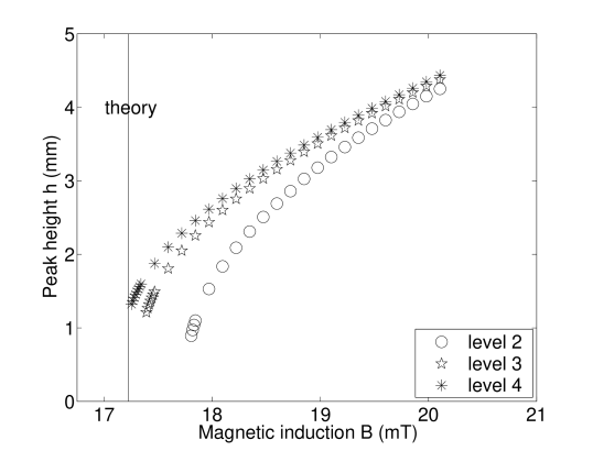
Figure 9: Peak height depending on the applied field strength for different refinement levels. The thin vertical line represents the critical induction of the instability (from the linear theory, see § 2.4).

Figure 9 shows the peak height as a function of the applied field for different refinement levels of the mesh for the underlying finite element method. The given peak height is the difference between the highest point on the surface, i.e. at the mid-point of a hexagonal cell, and the lowest point, i.e. at one of the corners of the hexagonal cell. Furthermore, the theoretical value for the onset of the instability is shown in Figure 9. We see that the qualitative behaviour is reproduced even on very coarse meshes. Obviously, one gets higher peaks on finer meshes. Moreover, we obtain numerically on the finest considered mesh a value for the critical magnetic induction which is very close to the theoretical value.

4 Results

In the experiment we recorded $540$ surface profiles in total, increasing and decreasing the magnetic induction in a quasistatic manner from $16.7\,\mathrm{mT}$ to $20.1\,\mathrm{mT}$ at maximum in steps of $0.015\,\mathrm{mT}$. Below this range, the surface remains flat apart from attraction of the fluid to the boundary of the container. Above this range the hexagonal pattern transforms into a square array of peaks which is not considered in the present paper.

In the next paragraphs, we will compare characteristic properties from these profiles to their counterpart from the simulated peaks. First we compare the amplitude of the pattern. Then we look at the wavenumber, and finally the full shape is examined.

4.1 Scaling behaviour of the amplitude

Figure 10: Pattern amplitude as a function of the magnetic induction. Triangles pointing upwards (downwards) represent the experimental data for an increasing (decreasing) magnetic field. The symbol size approximates the statistical error. For clarity only every 5th point is plotted. The connected circles show the simulation data. The thin vertical lines represent the numerically found transition points from (to) the flat surface. The thick solid line is a fit of the experimental data with the solution of an amplitude equation, the dashed line is representing the unstable branch of the solution. The inset reproduces the qualitative behaviour expected from the analysis by Gailitis (1977).

Figure 10 shows the amplitude of the pattern as a function of the applied magnetic induction, as defined in section 2.3. The triangles denote the experimental values where the size of the symbols has been chosen to approximate the statistical error of the data. The open circles represent the result from the simulations. The solid line is a fit of the experimental data with the solution of an amplitude equation from Friedrichs & Engel (2001). The root of the amplitude equation reads

$$A(\varepsilon)k_{c}=\frac{1}{2b_{1}}\left(b_{2}(1+\varepsilon)\pm\sqrt{b_{2}^{2}(1+\varepsilon)^{2}+4\varepsilon b_{1})}\right),$$ (16)

where $k_{c}=0.629\,\mathrm{mm^{-1}}$ is the critical wavenumber of equation (7) and $\varepsilon=(B^{2}-B_{c}^{2})/B_{c}^{2}$ is the bifurcation parameter. The fit parameters are

$$B_{c} =16.747\pm 0.001\,\mathrm{mT},$$ (17)

$$b_{1} =0.0889\pm 0.0001,$$ (18)

$$b_{2} =0.0873\pm 0.0003.$$ (19)

Using these parameters, the analytical function describes the measured data very well. However, it contains three adjustable parameters. The coefficients computed by Friedrichs & Engel (2001) are not applicable with our material parameters, because the expansion is only valid up to a susceptibility $\chi_{0}=1.05$. So the analytical theory has no predictive power for our fluid.

Let us now compare the measured amplitude with the results from the simulation which does not use a single adjustable parameter. Qualitatively, the numerical and experimental data compare very well. Both curves show a small bistable range, which makes it necessary to control the magnetic field in tiny steps to resolve the hysteresis. In the experiment, the width of the hysteresis loop is $0.17\,\mathrm{mT}$ whereas the numerical data expose a hysteretic range of $0.06\,\mathrm{mT}$. For a higher concentrated fluid ($\chi_{0}=2.2$), we have recently observed a larger hysteretic range of $1\,\mathrm{mT}$ using the same setup Richter & Barashenkov (2005). This indicates that for even smaller susceptibilities additional care has to be taken to resolve any hysteresis.

For both experimental and numerical data, the amplitude jumps at the critical point to a height of about $1.5\,\mathrm{mm}$ and reaches about $5\,\mathrm{mm}$ at the highest field. When decreasing the field, the surface pattern vanishes at the induction $B_{\ast}<B_{c}$ with a sudden drop from about $1\,$mm. Despite the principal similiarity of experimental and numerical results, the agreement is not convincing: at corresponding amplitudes the experimental data are shifted to lower fields.

(a)

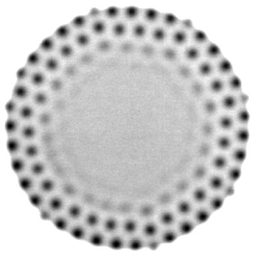
(b)

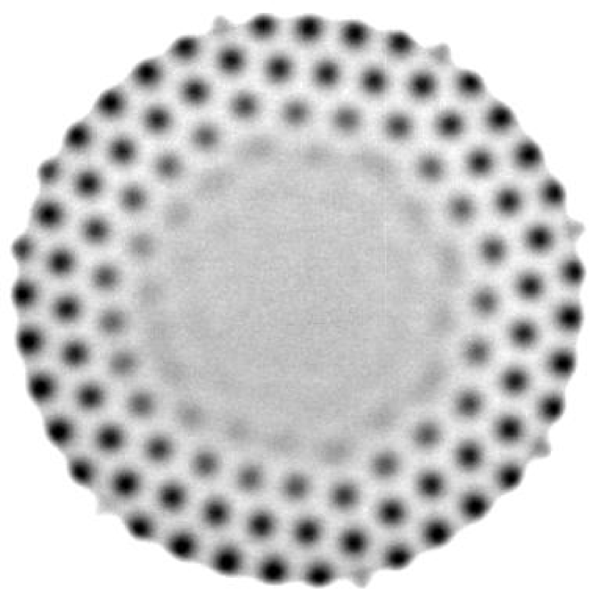
(c)

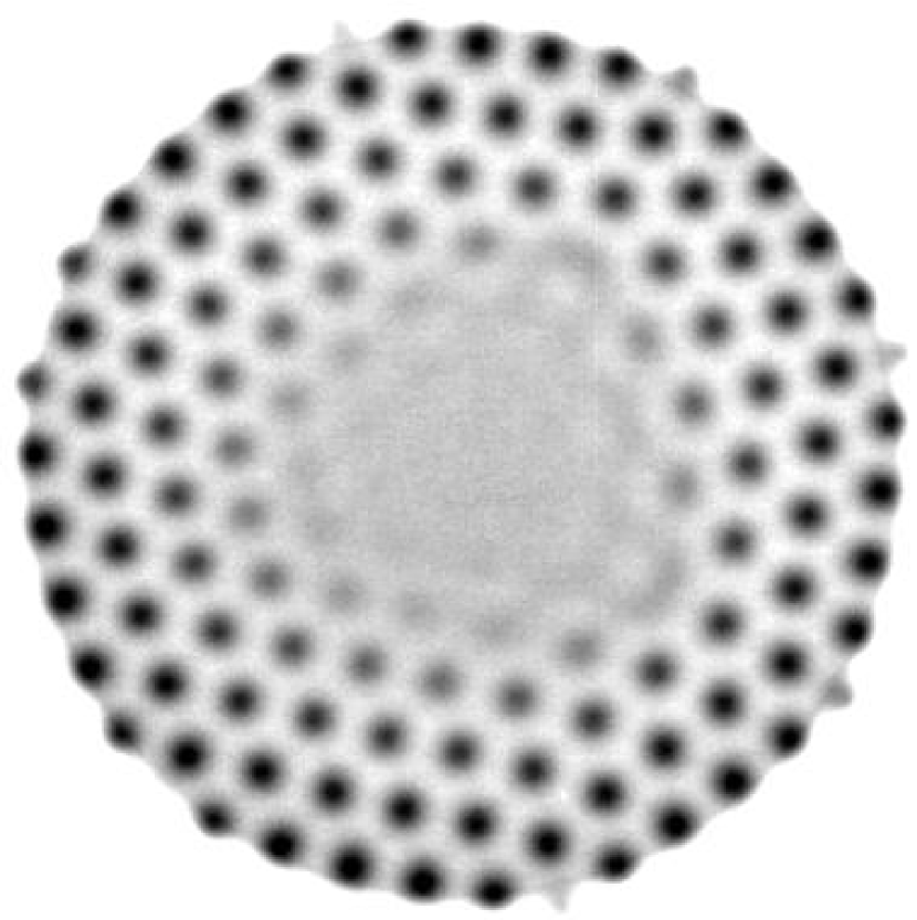
(d)

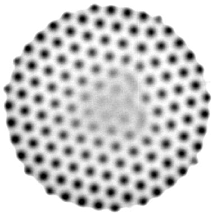
(e)

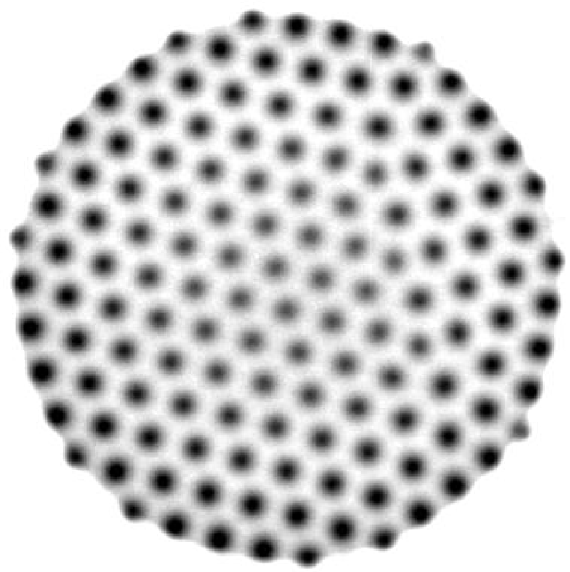
(f)

Figure 11: The pattern emerging as the magnetic induction is increased. The induction at the centre of the vessel is (a) $B=16.45\,\mathrm{mT}$, (b) $B=16.51\,\mathrm{mT}$, (c) $B=16.56\,\mathrm{mT}$, (d) $B=16.62\,\mathrm{mT}$, (e) $B=16.68\,\mathrm{mT}$, (f) $B=16.73\,\mathrm{mT}$.

The critical induction seen in the simulations $B_{c}^{\text{sim}}=17.25\,\mathrm{mT}$, i.e. the induction at which the jump occurs when increasing the field, is in accordance with the theoretical value from the linear stability analysis $B_{c}=17.22\,\mathrm{mT}$, see § 2.4. From the experimental data, the critical field can be extracted by the fit with equation (16), which yields $B_{c}=16.747\,\mathrm{mT}$. It deviates only by $3\,\%$ from the theoretical value. The difference between these two thresholds does not lie within the statistical error, which indicates that it is a systematic deviation: with the errors given in section 2.4, the uncertainty of the theoretical value $B_{c}$ is about $1.1\,\%$.

The imperfection induced by the edge of the bounded container has a great influence over the emerging pattern. Figure 11 shows six consecutive X-ray images for increasing magnetic induction. Because of the inhomogeneous magnetic induction over the vessel, pattern formation starts at the edge and expands towards the centre until the whole surface is covered with peaks.

Figure 12: Pattern amplitude as a function of the bifurcation parameter. $B_{c}$ has been chosen as 16.747 mT for the experimental data (from equation (17)) and 17.22 mT for the numerical data (from the linear theory). The simulation data are shown as a solid line only, whereas the experimental data are represented by the upward (downward) triangles for increasing (decreasing) magnetic field.

Nevertheless, the simulations can be reconciled with the experimental findings if we take the shift in the critical field into account. To see this, we plot both curves in a unifying diagram, see figure 12. Instead of the magnetic induction $B$, we plot the amplitude as a function of the bifurcation parameter $\varepsilon=(B^{2}-B_{c}^{2})/B_{c}^{2}$. Here, the actual $B_{c}$ is used for each data set. Now, the simulation data (plotted as a solid line only) match nearly perfectly the experimental data represented by the symbols. Slight deviations can be found near $\varepsilon=0$: for $\varepsilon>0$, the experimental amplitudes for decreasing and increasing field differ while the simulation produces identical results which fall somewhere in between these two curves. For $\varepsilon_{\ast}<\varepsilon<0$, i.e. in the range where the surface is bistable, the experiment already shows a small-amplitude surface pattern for increasing induction which should not be there in the ideal case.

The range of bistability observed in the experiment is about twice as wide as the one found in the simulation. Since the transition is not equally sharp due to the imperfection, it is not easy to determine the exact range where the surface is bistable.

4.2 The wavenumber modulus

Figure 13: Wavenumber of the experimental peak pattern, as determined from Fourier space. Triangles pointing downwards designate decreasing magnetic induction, upward triangles stand for rising induction. The dotted vertical line represents the critical induction from equation (17), the dashed line marks the critical wavenumber used in the simulations. The solid line is the preferred wavenumber taken from the theory by Friedrichs & Engel (2001), but computed for a different set of parameters (particularly, $\chi_{0}=0.35$), the linear extrapolation is dotted.

Figure 13 shows the experimental wavenumber for increasing and decreasing magnetic field which has been determined in the Fourier space with high precision (figure 4). Subpixel accurracy can be achieved due to the fact, that the Fourier space representation is a direct transform of the surface topography, not the transform of a flat photograph. Thus it includes the correct amplitudes. As the magnetic induction $B$ is increased, the wavenumber first increases and then decreases slowly. When $B$ is reduced afterwards, $k$ increases again, but to slightly smaller values; hence, $k$ exhibits a small hysteresis loop.

Friedrichs & Engel (2001) predict that the critical wavenumber of maximal growth $k_{c}$ should always be larger than the wavenumber of the resulting nonlinear pattern. However, in our experiment $k_{c}$ was found to be smaller than the wavenumber of the pattern, with the difference of the two being less than $3\,\%$. Further, the computed wavenumber decreases monotonically, as the magnetic induction is increased. In our experiment, instead, it has a maximum near the critical point. This also contradicts the findings of Bacri & Salin (1984) and Abou et al. (2001), which report a constant wavenumber. Note that the wavenumber measured here should not be confused with the wavenumber of maximal growth which is predicted by a linear stability analysis. This latter wavenumber shows a linear increase with $B$ as measured by Lange et al. (2000). During the nonlinear stabilization of the pattern, the wavenumber relaxes to some other value that is induced by the boundary conditions Lange et al. (2001). In all previous experiments the container had straight vertical edges corresponding to hard boundary conditions, which forces the wavenumber to be an integer multiple of the reciprocal container diameter. In contrast to that we equipped our container with a ramp that should give more freedom to the wavenumber. Such a ramp has been studied extensively e.g. in the context of convection by Rehberg et al. (1987). It is obvious from figure 13 that our ramp permits different wavenumbers for the same magnetic induction. Nonetheless the boundary seems to provide a soft pinning effect, which selects a wavenumber that is not necessarily the preferred one computed by Friedrichs & Engel (2001).

Because of the rather small difference between the experimentally found wavenumber and $k_{c}$, the wavenumber modulus $k$ has been fixed to the critical value $k_{c}=0.629\,\mathrm{mm^{-1}}$ (cf. § 2.4) in the simulations. In principle, a numerical ab initio estimation of the wavenumber of the pattern for each value of the induction is possible. This involves calculating the surface pattern for different preset wavelengths. Afterwards the preferred wavenumber can be selected by the minimum of the total free energy of the simulated profiles. However, the computational cost of this technique was too high at the present stage. Since the deviation of the experimental wavenumber from the critical one is only about $3\,\%$ at maximum, it is expected that the simulated profiles are a near match of the experiment.

4.3 The shape of the peaks

(a)

(b)

Figure 14: Comparison of experimentally (symbols) and numerically (solid lines) obtained peak profiles at $\varepsilon=0$ (a) and $\varepsilon=0.35$ (b)

Let us now consider the shape of the liquid crests. Figure 14 presents a direct comparison of the measured profile of a single peak selected from the centre of the dish with the shape of the peak obtained in the simulations. The diagram displays a diagonal cut through the unit cell from one corner to the opposite corner at two representative bifurcation parameters, $\varepsilon=0$ and $\varepsilon=0.35$. There is no adjustable parameter in this comparison, apart from centering the peak and normalizing to the wavelength. While the theoretical and experimental results differ near the critical value because of the imperfection, as discussed in section 4.1, the data show a perfect match at higher amplitudes ($\varepsilon=0.35$).

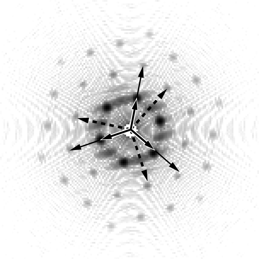
(a)

(b)

Figure 15: Analyzing the first three harmonics of the pattern. Figure (a) displays a logarithmic greyscale image of the Fourier transform at $B=20.1068\,\mathrm{mT}$. The wavevectors of the extracted harmonics are denoted by arrows. Figure (b) shows the corresponding amplitudes of the modes. Lines (symbols) mark experimental (computed) data, respectively. Solid thick lines and crosses represent basic modes, solid thin lines and circles modes of the form $2\boldsymbol{k}_{1}$, dashed lines and triangles modes of the form $\boldsymbol{k}_{1}-\boldsymbol{k}_{2}$.

For small amplitudes, it is expected that the pattern can be approximated by the dominating Fourier mode, i.e. a hexagonal pattern made up of three cosine waves:

$$A(\boldsymbol{x})=\frac{2}{9}\left(\cos\boldsymbol{k}_{1}\boldsymbol{x}+\cos\boldsymbol{k}_{2}\boldsymbol{x}+\cos\boldsymbol{k}_{3}\boldsymbol{x}\right)+\frac{1}{3}.$$

Here the wavevectors $\boldsymbol{k}_{1,2,3}$ enclose an angle of $120^{\circ}$, sum up to zero and have the same magnitude $k$. To give a quantitative measure to what extent the higher modes are important, we fit a hexagonal grid with the next two higher harmonics to both the experimental as well as the simulation data. The wavevectors are $\boldsymbol{k}_{1}-\boldsymbol{k}_{2},\boldsymbol{k}_{2}-\boldsymbol{k}_{3},\boldsymbol{k}_{3}-\boldsymbol{k}_{1}$ with the absolute value $\frac{k}{2}\sqrt{15}$ and $2\boldsymbol{k}_{1},2\boldsymbol{k}_{2},2\boldsymbol{k}_{3}$ with the absolute value $2k$. These vectors are displayed in figure 15 (a). Figure 15 (b) shows the dependence of the components on the bifurcation parameter. As expected, the basic Fourier mode is the largest component which contributes over $90\,\%$ even for the highest observed amplitude.

Since there is only a small amount of the higher harmonics, the shape of the peaks is mostly determined by the basic mode and thus should not vary much over the measured range. This can be seen directly if we rescale both the experimental and numerical data in a way that all peaks have the same width and height. In figure 16, we plot five different normalized peaks from the whole range. While the experimental values seem to match perfectly due to the noise, the numerical data exhibit a certain tendency to sharper peaks for an increasing field. However, this effect is very small, so the assumption of an invariant shape is a good approximation within the range $\varepsilon<0.44$.

(a)

(b)

Figure 16: The experimental (a) and numerically obtained (b) normalized profiles of different peaks show that the shape changes only slightly.

5 Discussion and Conclusion

We have studied experimentally and numerically the normal field instability in a ferrofluid. The qualitative features of this bifurcation can be described very well by the nonlinear theory of Friedrichs & Engel (2001). A quantitative comparison with this theory is not possible, because their approximations are only valid up to $\chi_{0}\approx 1$, which is exceeded by the initial susceptibility of our fluid $\chi_{0}=1.17$.

For a quantitative comparison we had to calculate the surface topography numerically by a finite element method. Our computations agreed with the measured amplitude to within $1\,\%$, provided that the uncertainties of the material parameters and geometrical imperfections were taken into account by matching the critical induction $B_{c}$. This indicates that a fluid as complex as magnetic liquids can be indeed described well by the set of three basic equations, the Navier–Stokes equation, the Maxwell equation and the Young–Laplace equation. It turned out to be essential to include the experimentally obtained magnetization curve.

In an attempt to measure the preferred wavenumber – namely the one minimizing the free energy – in the nonlinear regime, we have introduced somewhat softened boundary conditions in the form of a ramp, which allows for smooth variation of the wavenumber as a function of the magnetic field. It turned out that this ramp stabilizes wavenumbers above the critical value of $k_{c}$, while the theory by Friedrichs & Engel (2001) predicts the preferred number to be below $k_{c}$. Whether a ramp can be constructed which selects the preferred wavenumber, remains to be investigated in the future.

Because the radioscopic measurement technique allows us to investigate the full profile of the peaks, we are able to quantify the ratio of the fundamental mode to the higher harmonics under variation of $B$. It turned out, that the higher harmonics contribute less than $10\,\%$ in a range up to $\varepsilon=0.44$. This is an encouraging result for further analytical treatment of the problem in terms of amplitude equations for the first few modes. Whether the contribution of higher harmonics remains small for fluids with higher susceptibility, where already visual inspection reveals sharper peaks, remains a topic of further investigations.