Delay Induced Oscillations in a Fundamental Power System Model

Abstract

In this paper, we study the dynamics and stability of a fundamental power system model when a time delay is imposed on the excitation of the generator. It is observed that sustained oscillations can arise in an otherwise stable power system through a delay induced Andronov-Hopf bifurcation. Numerical simulations are conducted to explore the dynamics of the time delayed system after the bifurcation which indicate period doublings culminating in a strange attractor.

1 Introduction

Complex nonlinear phenomena in power system models have been extensively studied in the past. Arnold diffusion, [1] and chaotic motions, [2] have been studied in power system models described by the swing equations. The classic period doubling bifurcation route to chaos has been studied in a three node power system model, [3] using simplified models for the generator [4],[5],[6],[7] and later, with detailed generator models in [8]. Hard-limit induced chaotic behavior in a single machine infinite bus formulation was studied in [9] by extensive numerical simulations where it was argued that the interaction of hard limits and system transients led to sustained chaotic behavior. In [10], hard limits were approximated by a smooth function to study bifurcations in the three node power system as an extension of [8].

While considerable attention ([1]-[10]) has been devoted to the study of power system models in the absence of time delays, not as much attention has been paid to understand power system dynamics in the presence of time delays with the exception of [11]. In modern power systems with digital control schemes, the acquisition, filtering and processing of signals can lead to possible time delays, [11]. In [11], the authors demonstrated an effective control technique using prediction to compensate for the delay in generator excitation. In the deregulated power industry, communication delays arising from the use of phasor measurement units in wide area measurement systems could contribute to time delays in the acquisition of control signals. Thus, the focus of this paper is to study the effect of a time delay on the dynamics of a representative power system model.

A Single Machine Infinite Bus (SMIB) system consisting of a generator interfaced to the grid through a transmission line, Figure 1 is considered in this study. The SMIB system ([12],[13]) has served as a long standing paradigm to understand the dynamics of a single generator when connected to a large power system. The simplicity of the SMIB system facilitates analysis and thereby enables one to gain insight in to the dynamic behavior of a synchronous generator. The electro-mechanical equations of the generator are described by the standard flux-decay model and the excitation is represented by a single time constant system, Figure 2. The excitation voltage $E_{fd}$ is subject to a time delay $\tau$. The dynamics of the resultant system is then described by delay differential equations (DDEs). The reader is referred to [14], [15] for the general theory of DDE systems. In power system models described by ODEs, Hopf bifurcations usually arise when the loading of the generator, or control gains exceed certain critical values, [13]. However as remarked earlier, little attention (with the exception of [11]) has been paid to study power system models with delays. Therefore, we focus on understanding the role of a time delay on the dynamics of a synchronous generator. Later on, we show that even if the control gain and generator loadings are chosen to obtain a stable operating point, a critical delay in the excitation can cause the normally stable equilibrium to become unstable.

Figure 1: Single Machine Infinite Bus System

Figure 2: Excitation Control System

2 System Model

The system shown in Figure 1 illustrates a standard single machine infinite bus (SMIB) system equipped with a fast acting static excitation system (indicated by ‘Exc’). Assuming a single time constant model for the excitation system shown in Figure 2 and the flux decay model for the generator, the dynamics of the single machine system in the presence of a time delay in excitation ($E_{fd}$) can be described by,

$\Sigma_{\tau}$ :

$$\dot{\delta}=\omega_{b}\overline{\omega}$$ (1)

$$\dot{\overline{\omega}}=\frac{(P_{m}-P_{e})}{2H}$$ (2)

$$\dot{E^{{}^{\prime}}_{q}}=\frac{-E_{q}+(x_{d}-x^{{}^{\prime}}_{d})i_{d}+E_{fd}(t-\tau)}{T^{{}^{\prime}}_{do}}$$ (3)

$$\dot{E_{fdx}}=\frac{-E_{fdx}+K_{A}(V_{ref}-V_{t})}{T_{A}}$$ (4)

$$E_{fd}=\left\{\begin{array}[]{ll}E_{fdx}&\mbox{if $E_{fd}^{min}\leq E_{fdx}\leq E_{fd}^{max}\ $}\\ E_{fd}^{min}&\mbox{if $E_{fdx}\leq E_{fd}^{min}\ $}\\ E_{fd}^{max}&\mbox{if $E_{fdx}\geq E_{fd}^{max}\ $}\end{array}\right.$$ (8)

(8), describes a limiter which imposes upper ($E_{fd}^{max}$) and lower ($E_{fd}^{min}$) limits on the excitation voltage $E_{fd}$ of the synchronous machine. While the effect of excitation limits on the system dynamics and bifurcations has been previously studied in [9] and [10], the aim of the present paper is to understand the role of the delay term $\tau$. Therefore, in the rest of the analysis which demands smoothness of the models, the excitation limits are ignored which implies that $E_{fdx}=E_{fd}$. The rest of the variables $(v_{d},i_{d},v_{q},i_{q}$) are given by,

$$i_{d}=\frac{\cos(\delta)-E^{{}^{\prime}}_{q}}{x^{{}^{\prime}}_{d}+x_{e}},\;\;i_{q}=\frac{\sin(\delta)}{x_{q}+x_{e}}$$ (9)

$$v_{d}=-\frac{x_{q}\sin(\delta)}{x_{q}+x_{e}},\;\;v_{q}=\frac{x^{{}^{\prime}}_{d}\cos(\delta)-E^{{}^{\prime}}_{q}}{x^{{}^{\prime}}_{d}+x_{e}}$$ (10)

The electrical power $P_{e}$ and terminal voltage $V_{t}$ are expressed in terms of the state variables from,

$$P_{e}=v_{d}i_{d}+v_{q}i_{q},\;\;V_{t}=\sqrt{v^{2}_{d}+v^{2}_{q}}$$ (11)

3 Local Stability

The local asymptotic stability of the equilibrium point for the system can be studied from the roots of the characteristic polynomial corresponding to the linearisation of $\Sigma_{\tau}$ given by

$$|\lambda I-A|=0$$ (12)

where,

$$A=\left[\begin{array}[]{cccc}0&\omega_{b}&0&0\\ -\frac{K_{1}}{2H}&0&-\frac{K_{2}}{2H}&0\\ -\frac{K_{4}}{T^{{}^{\prime}}_{do}}&0&-\frac{1}{K_{3}T^{{}^{\prime}}_{do}}&e^{-\lambda\tau}/{T^{{}^{\prime}}_{do}}\\ -\frac{K_{A}K_{5}}{T_{A}}&0&-\frac{K_{A}K_{6}}{T_{A}}&-\frac{1}{T_{A}}\end{array}\right]=0$$ (13)

In the linearisation of a single machine system expressed in (13), the parameters $K_{1},\dots K_{6}$ are known as Heffron-Phillips constants, [12], [13] which depend on the equilibrium and the machine parameters (see Appendix A). Substituting for $A$ from (13) in to (12) yields the characteristic polynomial for the system which can be expressed as

$$f_{\tau}(\lambda)=f_{1}(\lambda)+e^{-\lambda\tau}g_{1}(\lambda)=0$$ (14)

where,

$$f_{1}(\lambda)=\lambda^{4}+\lambda^{3}\beta_{1}+\lambda^{2}\beta_{2}+\lambda\beta_{3}+\beta_{4}$$ (15)

$$g_{1}(\lambda)=\lambda^{2}\beta_{5}+\beta_{6}$$ (16)

The coefficients $\beta_{1},\dots\beta_{6}$ are given by,

$$\beta_{1}=K^{\prime}_{3}+1/T_{A}$$ (17)

$$\beta_{2}=K^{\prime}_{3}/T_{A}+K^{\prime}_{1}\omega_{b}+K^{\prime}_{6}/T^{{}^{\prime}}_{do}$$ (18)

$$\beta_{3}=\omega_{b}(K^{\prime}_{1}K^{\prime}_{3}-K^{\prime}_{2}K^{\prime}_{4})+K^{\prime}_{1}\omega_{b}/T_{A}$$ (19)

$$\beta_{4}=\omega_{b}(K^{\prime}_{1}K^{\prime}_{3}-K^{\prime}_{2}K^{\prime}_{4})$$ (20)

$$\beta_{5}=K^{{}^{\prime}}_{6}T^{{}^{\prime}}_{do}$$ (21)

$$\beta_{6}=\omega_{b}(K^{\prime}_{1}K^{\prime}_{6}-K^{\prime}_{2}K^{\prime}_{5})/T^{{}^{\prime}}_{do}$$ (22)

with

$$K^{\prime}_{1}=K_{1}/2H,\;K^{\prime}_{2}=K_{2}/2H,\;K^{\prime}_{3}=1/K_{3}T^{{}^{\prime}}_{do},$$

$$\;K^{\prime}_{4}=K_{4}/T^{{}^{\prime}}_{do},\;K^{\prime}_{5}=K_{A}K_{5}/T_{A},\;K^{\prime}_{6}=K_{A}K_{6}/T_{A}$$

In the absence of delay, by setting $\tau=0$ in (14) we note that the characteristic polynomial is described by $f_{0}(\lambda)=f_{1}(\lambda)+g_{1}(\lambda)=0$. In the present study, the control gain, machine loading and other parameters are chosen so that the equilibrium point of the system without delay is locally asymptotically stable. With this assumption, the coefficients $\beta_{i},i=1\dots 6$ are all positive for typical values of machine parameters and loading conditions. In the following section, we shall study the local stability of the equilibrium as the delay $\tau$ is varied.

4 Delay Induced Oscillations

Local stability of the equilibrium point of $\Sigma_{\tau}$ is governed by the roots of the characteristic polynomial $f_{\tau}(\lambda)=0$, (14). Continuous dependence of the roots of (14) on $\tau$ implies that there exists $\tau_{c}$ such that $\Re e\{{\lambda}\}<0$ when $\tau\in[0,\tau_{c})$. A loss of asymptotic stability of the equilibrium occurs when $\Re e\{{\lambda}\}=0$ for some critical value of $\tau=\tau_{c}>0$. Suppose the characteristic polynomial (14) has a pair of purely imaginary roots $\lambda=\pm i\omega_{c}$ when $\tau=\tau_{c}$, we get

$$f_{1}(i\omega)+e^{-i\omega\tau}g_{1}(i\omega)=0$$ (23)

Substituting for $f_{1}(.)\;$and $g_{1}(.)$ from (15) and (16) we get,

$$\beta_{c}+\beta_{a}\cos(\omega\tau)=0$$ (24)

$$\beta_{b}-\beta_{a}\sin(\omega\tau)=0$$ (25)

where,

$$\beta_{a}=\beta_{6}-\omega^{2}\beta_{5}$$ (26)

$$\beta_{b}=\omega\beta_{3}-\beta_{1}\omega^{3}$$ (27)

$$\beta_{c}=\omega^{4}-\omega^{2}\beta_{2}+\beta_{4}$$ (28)

From (24) and (25), the pair ($\omega_{c},\tau_{c}$) for which the system (14) has a pair of purely imaginary roots can be found from

$$\beta_{a}^{2}=\beta_{b}^{2}+\beta_{c}^{2}$$ (29)

$$\tan(\omega\tau)=-\frac{\beta_{b}}{\beta_{c}}$$ (30)

By implicit differentiation of (14), we get

$$\frac{d\lambda}{d\tau}=\frac{\lambda e^{-\lambda\tau}g_{1}(\lambda)}{f^{\prime}_{1}(\lambda)+g^{\prime}_{1}(\lambda)-\tau e^{-\lambda\tau}g_{1}(\lambda)}$$ (31)

Setting $\lambda=i\omega_{c}$ and $\tau=\tau_{c}$ in (31), using (29), (30) and simplifying the terms yields

$$\sigma=\Re e\{\frac{d\lambda}{d\tau}\}|_{\tau_{c},\omega_{c}}=\frac{2\omega_{c}\beta_{a}(\beta_{2}-\beta_{5})}{D^{2}}$$ (32)

where,

$$D^{2}=D_{a}^{2}+D_{b}^{2}$$ (33)

$$D_{a}=\beta_{3}-3\beta_{1}\omega_{c}^{2}-\beta_{a}\tau_{c}\cos(\omega_{c}\tau_{c})+2\omega_{c}\beta_{2}\sin(\omega_{c}\tau_{c})$$ (34)

$$D_{b}=2\omega_{c}\beta_{2}-4\omega^{3}_{c}+\beta_{a}\tau_{c}\sin(\omega_{c}\tau)+2\omega_{c}\beta_{2}\cos(\omega_{c}\tau_{c})$$ (35)

Therefore, the sign of $\sigma$ is governed by the terms in the numerator of (32). Substituting for the terms $\beta_{2},\beta_{5}$ from Appendix B we get,

$$\beta_{2}-\beta_{5}=\frac{1-K_{3}T_{e}K_{6}}{T^{{}^{\prime}}_{do}K_{3}T_{e}}+\frac{K_{1}\omega_{b}}{2H}$$ (36)

Under normal operating conditions for a power system, the Heffron-Phillips constants satisfy,

$$K_{1}>0$$ (37)

$$0<K_{3}<1$$ (38)

$$0<K_{6}<1$$ (39)

In addition, fast acting excitation systems typically have a small time constant so that $0<T_{e}<1$. In view of the above conditions, we note that

$$(\beta_{2}-\beta_{5})>0$$ (40)

The equations for $\beta_{a}(\omega_{c})\neq 0$ turn out to be complicated, making explicit analysis difficult. However numerical solutions of (29) over realistic ranges of operating conditions yield nonzero values for the term $\beta_{a}$ at the critical point in which case, $\sigma>0$. Therefore, the results of the analysis so far can be summarized in the following proposition.

Proposition 1 : The system $\Sigma_{\tau}$ satisfies the sufficient conditions for a delay induced Andronov-Hopf-bifurcation under the following assumptions.

• ] the system without delay $\Sigma_{0}$ is stable $\Rightarrow f_{0}(\lambda)=0$ has no roots on the right half plane.

• ] if $\tau\neq 0$, then $\lambda=0$ is not a root of $f_{\tau}(\lambda)$ (14).

The assumptions [A1] and [A2] indicate that at the critical point, the characteristic polynomial has a purely imaginary pair of roots and all other roots of the polynomial have strictly negative real parts. The delay induced loss of operating point stability leads to the emergence of periodic solutions. The stability of the resulting periodic motion can be inferred from the sign of a certain quantity which proves to be too difficult in this case. Therefore, we resort to numerical simulations in the following section to study the dynamics of the system after delay induced instability.

5 Simulation Results

All numerical integrations were carried out using dde23 in MATLAB. A numerical simulation of the system $\Sigma_{\tau}$ is shown in Figure 3 assuming typical values for the machine loading and control gain $K_{A}$ (supplied in Appendix A) that results in a stable operating point in the absence of delay. Then the delay $\tau$ is increased gradually from zero up to the critical value $\tau_{c}$ when the equilibrium point loses stability. The rotor angle $\delta$ is plotted in all time domain simulations. The transition from damped oscillations (when $0<\tau<\tau_{c}$) to sustained oscillations (when $\tau>\tau_{c}$) can be noted from Figure 3. Incidentally, the solution of (29) and (30) yield $\tau_{c}=0.0533$ which closely matches the critical delay observed by simulation, i.e. $\tau_{cri}=0.055$. When the delay $\tau$ is increased further, a period doubling (upper panel of Figure 4) is noticed which eventually culminates in a strange attractor (lower panel of Figure 4).

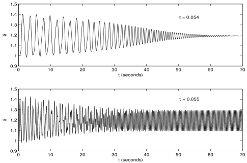
Figure 3: The onset of oscillatory activity in the time delayed SMIB system. The critical delay $\tau_{c}=0.055$. Upper panel shows a stable trajectory when $\tau=0.054<\tau_{c}$. Lower panel shows sustained oscillations when $\tau=\tau_{c}$.

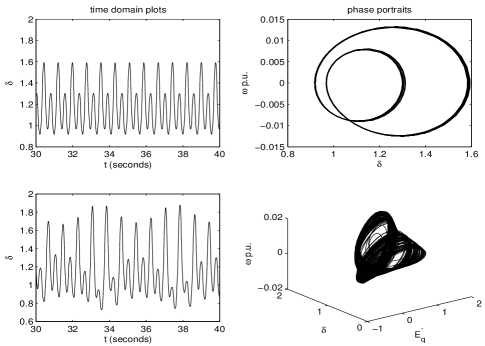
Figure 4: Simulation of system trajectory beyond $\tau_{c}$. Upper panel indicates a period doubling when $\tau=0.059$ followed by a strange attractor in the lower panel when $\tau=0.061$.

6 Conclusions

Power system models are capable of displaying a rich variety of nonlinear phenomena which have been formally studied by bifurcation theory. In particular, the emergence of oscillations in power system models has been attributed to Hopf bifurcations which have been shown to arise when the control gains or machine loading exceed critical values. In this paper, the dynamics of a fundamental power system model is studied when the field voltage of the generator is subject to a time delay. It is shown by preliminary analysis that a nominally stable operating point can be destabilized when the time delay exceeds a critical value $\tau_{c}$ through a Andronov-Hopf bifurcation. The behavior of the system for $\tau>\tau_{c}$ is further studied by numerical simulations which indicate that the system undergoes a period doubling which eventually culminates in a strange attractor. Further analysis to determine the bifurcations of the ensuing limit cycle would be an interesting subject for future research.

Appendix A

The Heffron-Phillips constants for a lossless network are given by

$$K_{1}=\frac{E_{qo}\cos(\delta_{o})}{(x_{e}+x_{q})}+\frac{(x_{q}-x_{d}^{\prime})i_{qo}\sin(\delta_{o})}{x_{e}+x^{\prime}_{d}}$$ (41)

$$K_{2}=\frac{\sin(\delta_{o})}{x_{e}+x^{\prime}_{d}},\;\;K_{3}=\frac{x_{e}+x^{\prime}_{d}}{x_{d}+x_{e}}$$ (42)

$$K_{4}=\frac{(x_{d}-x^{\prime}_{d})\sin(\delta_{o})}{x_{e}+x^{\prime}_{d}}$$ (43)

$$K_{5}=\frac{-x_{q}v_{do}\cos(\delta_{o})}{(x_{e}+x_{q})V_{to}}-\frac{-x^{\prime}_{d}v_{qo}\sin(\delta_{o})}{(x_{e}+x^{\prime}_{d})V_{to}}$$ (44)

$$K_{6}=\frac{x_{e}v_{qo}}{V_{to}(x_{e}+x^{\prime}_{d}})$$ (45)

where the subscript ‘$o$’ indicates the values of the variables at the equilibrium point which can be solved by setting (1)- (4) to zero.

Appendix B

System Parameters :
$x_{d}=1.79,\;x_{q}=1.71,\;x^{\prime}_{d}=0.169,\;P_{m}=0.9,\;T^{\prime}_{do}=4.3,\;H=5,\;\omega_{b}=377,\;x_{e}=0.4,\;\;R_{e}=0$.

Exciter Parameters :
$K_{A}=200,\;T_{A}=0.05$.

References

[1]
F. M. A. Salam, J. Marsden and P. P. Varaiya, “Arnold diffusion in
swing equations of a power system”, IEEE Trans. on Circuits and
Systems, 30(8), 199-206 (1984).
[2]
N. Kopell and R. B. Washburn, “Chaotic motions in the two degrees
of freedom swing equations”, IEEE Trans. on Circuits and Systems,
29(11), 738-746 (1982).
[3]
I. Dobson and H. D. Chiang, “Towards a theory of voltage collapse
in electric power systems”, Sys. Cont. and Lett., 13, 253-262
(1989).
[4]
E. H. Abed, H. O. Wang, J. C. Alexander, A. M. A. Hamdan and H. C.
Lee, “Dynamic bifurcations in a power system model exhibiting
voltage collapse”, Int. J. Bifurcations and Chaos, 3(5)
1169-1176 (1993).
[5]
C. W. Tan, M. Varghese, P. P. Varaiya and F. W. Wu, “Bifurcation,
chaos and voltage collapse in power systems”, Proc. IEEE, 83(11), 1484-1496 (1995).
[6]
H. D. Chiang, C. W. Liu, P. P. Varaiya, F. W. Wu and M.G. Lauby,
“Chaos in a simple power system”, IEEE Trans. on Power Systems,
8(4) 1407-1417 (1993).
[7]
H. O. Wang, E. H. Abed and A. M. A. Hamdan, “Bifurcations, chaos
and crises in voltage collapse of a model power system”, IEEE Trans.
Circuits and Systems I, 41(3) 294-302 (1994).
[8]
Rajesh G. Kavasseri and K. R. Padiyar, “Bifurcation analysis of a
three node power system with detailed models”, Int. J. of Electrical
Power and Energy Systems, 21 375-393 (1999).
[9]
W. Ji and V. Venkatasubramanian, “Hard limit induced chaos in a
fundamental power system model”, Int. J. of Electrical Power and
Energy Systems, 18(5), 279-295 (1996).
[10]
Rajesh G. Kavasseri and K. R. Padiyar, “Analysis of Bifurcations in
a Power System Model with Excitation Limits”, Int. J. of
Bifurcations and Chaos, 11(9), 2509-2517 (2001).
[11]
G. A. Martin, M. M. Begovic and D. G. Taylor, “ Transient Control
of Generator Excitation in Consideration of Measurement and Control
Delays”, IEEE Trans. on Power Delivery, 10(1), 135-141 (1995).
[12]
P. M. Anderson and A. A. Fouad, Power System Control and
Stability, ( The Iowa State Press, Ames, Iowa, 1977).
[13]
K. R. Padiyar, Power System Dynamics and Control, (John Wiley,
Singapore, 1996).
[14]
J. K. Hale, Theory of functional differential equations,
(Spring-Verlag, New York, 1977).
[15]
R. E. Bellman and K. L. Cooke, Differential Difference
Equations (Academic Press, New York , 1963).