Correlations and periodicities in Himalayan tree ring widths and temperature anomalies through wavelets

Abstract

We have studied periodicities and correlation properties of tree ring width chronology of deodar tree from Joshimath (1584 - 1999 years) and Uttarkashi (1500 - 2002 years) in the western Himalayas and the pre-monsoon (March-April-May) temperature anomalies (1876 - 2003) relative to 1961 -1990 mean, through wavelet analysis. Periodic behavior is observed in the tree ring chronology with periodicity in the form 11, 22, and 42 years. The analysis of the self-similar nature reveals long-range correlation with a Hurst exponent, $H>0.5$. These are anti-correlated with the temperature anomalies. An interesting inversion behavior is observed around the year $1750$. The power spectral analysis of the time series corroborate the results of wavelet method.

I Introduction

Our understanding of the variability of climate is largely hampered by limited length of instrumental weather records, spanning in most cases to past 100 years. High-resolution proxy climate records, with precise dating control, provide very good tool to supplement the weather records back by several centuries and millennia. Of these records, tree rings provide valuable proxy as annual growth rings can be precisely dated to calendar year of their formation and the overlapping template of tree ring chronologies can be calibrated with weather data to hindcast the climate variables. Such long-term records can be used to understand the mode of climate variability in a longer perspective.

The climate dynamics is affected by a large number of factors, which in turn is reflected on a variety of proxy records, such as tree ring widths, ocean and lake deposits etc. The tree ring data has a much higher resolution as compared to the later ones. Recently, these two class of data have been combined through the multi-resolution capability of the wavelets mob , for reconstructing millennial-scale climate variability, in the northern hemisphere. Multi-centennial variations in temperature, possibly arising out of natural phenomena, have been inferred from the above study, which correlates well with a general circulation model. The variations in temperature naturally introduces variations in precipitation patterns, which are truthfully recorded in the tree ring data. At present, global temperatures are increasing; the last century in particular has seen substantial variations in temperature and precipitation rates, which may be arising due to anthropogenic forcing or natural causes.

The goal of the present article is to employ wavelet transform for studying ring chronologies’ periodicities in tree ring and detect the presence of self-similar behavior and correlation properties mandel ; feder . The fact that, a number of phenomena in nature reveal these type of behavior and wavelets provide an ideal tool to find the same, motivates this study. Apart from the implications of the periodicities, the nature of the self-similar fractal behavior, in terms of persistence or anti-persistence will carry long-term physical implication.

In the following section, we outline briefly the basic properties of the wavelet transform which are useful for the present analysis. In section III, a description is provided about the tree ring materials, chronology preparation and climate data. Sec. IV deals with results and discussions. We finally conclude in sec. V with a summary and future directions of work.

II Wavelet Transform

Since the early eighties, wavelet transform has emerged as a powerful tool to analyze transient and time-varying phenomena daub ; mall . It has innumerable applications in various fields, ranging from signal processing, natural sciences, economics and finance data analysis chu ; ding ; arn1 ; mani1 ; mani2 ; mani3 ; mani4 ; pkp1 ; pkp2 . Wavelet transform decomposes an input signal into components that depend on position and scale. We can characterize the input signal by changing the scale for a particular location.

The wavelet basis functions are localized both in time and frequency (or position and scale). The wavelets are parameterized by the scale parameter (dilation parameter) $s>0$, and a translation parameter $-\infty<a<\infty$, thus the wavelet basis can be constructed from one single function $\psi(x)$ according to

$$\psi_{s,a}(x)=\psi(\frac{x-a}{s}).$$ (1)

Here, $\psi(x)$ is the mother wavelet. Given a function $f(x)$, the (continuous) wavelet transform is defined as

$$W[f](s,a)=\frac{1}{\sqrt{s}}\int_{-\infty}^{+\infty}\psi_{s,a}^{*}f(x)dx.$$ (2)

Here $\psi^{*}(x)$ denotes the complex conjugate of $\psi(x)$. In order for a function $\psi(x)$ to be usable as an analyzing wavelet, one must demand that it has zero mean. We make use of continuous Morlet wavelet for studying the periodicity in our data. The behavior of the global power spectrum is inferred from $ln|W_{s,a}[f]|^{2}$ versus scale $s$.

We employ the Daubechies wavelets for finding the self similar behavior of the time series. In order to be useful for removing polynomial trends, wavelets belonging to the Daubechies family are made to satisfy,

$$\int_{-\infty}^{+\infty}x^{m}\psi(x)dx=0,~{}~{}0\leq m\leq n.$$ (3)

Here the upper limit n is related to what is called the order of the wavelet. We use Daubechies-12 wavelet to find the Hurst exponent (H), making use of the average wavelet coefficient method awc . This wavelet has been found to be reliable through calculating Hurst exponent for the time series like Gaussian white noise and binomial multifractal model, for which the Hurst exponent is known mani5 .

In the average coefficient method for estimating the correlation behavior, one computes,

$$W[f](s)=\langle|W[f](s,a)|\rangle\simeq s^{1/2+H}.$$ (4)

W[f](s) is the averaged wavelet energy of all locations for different scales. Thus for the given time series, the scaling exponent (1/2 + H) is measured from the log-log plot of W[f](s) versus scale $s$ through linear fit. The Hurst exponent (H) varies between $0<H<1$. If $H<1/2$, the time series possesses anti-correlation behavior and for $H>1/2$ long-range correlation behavior is present. For uncorrelated time series, $H=1/2$. We have also analyzed the time series through Fourier power spectral analysis, where $P(f)\sim f^{-\alpha}$, and $\alpha=2H+1$.

III Tree ring materials and chronology preparation

Tree ring samples in the form of increment cores were collected from Himalayan cedar trees growing at moisture stressed sites in Juma near Joshimath and Gangotri in Uttarkashi. Increment borers were used to extract 4mm diameter cores from trees at 1.4m stem height from ground. The increment cores were processed to cross date the sequence of growth rings in trees to exact calendar year of their formation. The ring widths of precisely dated growth rings were measured using linear encoder with the accuracy of 0.01mm. Long-term growth trends inherent in trees due to increasing age and stem girth were removed by standardizing the ring width measurement series. Individual tree ring width measurement series were fitted with negative exponential or linear regression line with negative slope or no slope and indices calculated as quotient of actual measurement and curve value. The individual tree series after standardization were averaged using bi-weight robust estimation of the mean to develop mean chronology using program ARSTAN. The chronology dynamics assumed to be climate driven could be used to examine the possible low frequency modes and how these might have varied over time jay1 ; ram ; jay2 . The tree ring series prepared form Gangotri, Uttarkashi and Jurna, Joshimath in Uttaranchal are shown in Figs. 1 and 2 respectively.

Climate data: Tree ring chronologies showed strong negative relationship with pre-monsoon temperature. To calibrate the tree ring series, we prepared mean pre-monsoon temperature series by merging temperature anomalies of nine stations (relative to 1961 - 1990 mean) in western Himalaya. The mean temperature series (Fig. 7) is biased by larger station data records beginning from the mid of $20^{th}$ century except in case of four stations, where it extends back to beginning of the $20^{th}$ century and even earlier.

IV Results and Discussion

As mentioned earlier, we make use of the Morlet wavelet for studying the periodicity in the data. The average wavelet coefficient method is used for finding the correlation behavior through calculation of Hurst exponent. It is worth mentioning that, here we are dealing with non-stationary data; wavelets are well suited for the analysis of this class of data. The wavelet coefficients are investigated and wavelet amplitude spectrum is obtained.

Figs. 1 and 2 depict the global power spectra of the tree data from Uttarkashi and Joshimath, clearly revealing multiple periodic variations at 11, 22, and 42 years respectively nara . Fig. 3, depicts the global power spectrum of temperature records, which shows an anti-correlation behavior with the tree ring variations of Figs. 1 and 2. Scalogram of the wavelet coefficients is given in Fig. 4; where one can observe the periodicities as mentioned earlier. An interesting inversion is clearly seen around 1570 years.

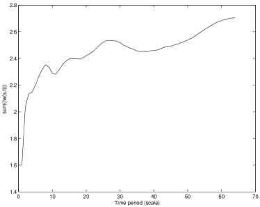
Figure 1: The semi-log plot of wavelet power summed over all time at different scales (time period). One clearly observes the variations at $11$, $22$ and $42$ years.

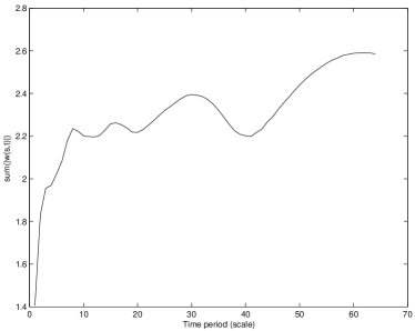
Figure 2: the semi-log plot of wavelet power summed over all time at different scales (time period). Here also one sees the variations at $11$, $22$ and $42$ years.

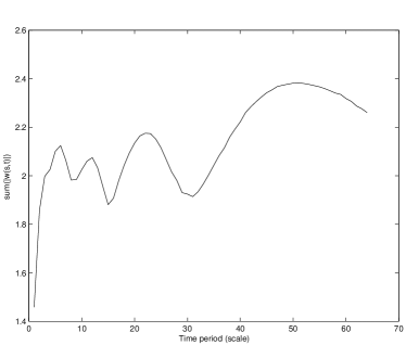
Figure 3: The semi-log plot of the wavelet power versus scale (time period) for the temperature data. An anti-correlation behavior with the tree ring variations of Figs. $1$ and $2$ is clearly seen.

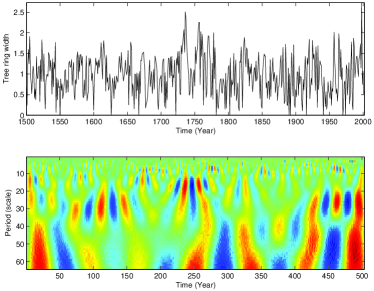
Figure 4: (Upper panel) time series of ring width chronology of deodar from Uttarkashi and (lower panel) scalogram of the above time series, one can clearly see the inversion around 1570 year and the periodicities as mentioned above.

In Figs. 5, 6 and 7, upper panel (a) shows the time series of accumulated tree ring and temperature data after subtracting the mean, whereas (b) shows the power law behavior of the Fourier spectral analysis of the time series.

Figure 5: Power spectral analysis for ring width chronology of deodar from Uttarkashi, yielding the scaling exponent $\alpha=2.45066$.

Figure 6: Power spectral analysis for ring width chronology of deodar from Joshimath, giving the scaling exponent $\alpha=2.4416$.

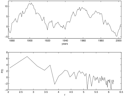
Figure 7: Power spectral analysis for pre-monsoon temperature, giving the scaling exponent $\alpha=2.34$.

We now investigate the correlation properties of tree ring time series, for which we have used average wavelet co-efficient method. Hurst exponent, which is a measure of correlation properties in a time series is computed through Daubechies-12 wavelet. We have found that the tree ring time series possess long range correlation, the Hurst exponent $H\sim 0.73$ (tree ring series from UttarKashi), $H\sim 0.74$ (tree ring series from Joshimath) and for temperature anomalies $H\sim 0.7$. The results obtained from average wavelet coefficient method is comparable with the Fourier power spectral analysis $P(s)~{}s^{-\alpha}$ results by the relation $\alpha=2H+1$, keeping in mind the finite data length. The obtained scaling exponent through Fourier analysis is $\alpha=2.45066,H\sim 0.73$ (tree ring series from Uttarkashi) and $\alpha=2.4416,H\sim 0.72$ (tree ring series from Joshimath). Temperature record yields a scaling exponent $\alpha=2.34$ and the corresponding Hurst exponent $H\sim 0.67$. This also shows long range correlation behavior.

V Conclusion

From the above obtained results one can clearly see the climate variations in both time and frequency scales. One observes both periodic and self-similar processes. Keeping in mind the non-stationary nature of the time series, the efficacy of the wavelets in extracting the above behavior is clearly seen. This is due to the localization and multi-resolution ability of the wavelets. As expected, there is an anticorrelation between the tree-widths and temperature anomalies. Surprisingly, the self-similar behavior yields long-range correlation. This aspect needs to be further studied carefully in conjunction with other related data sets, since long-range correlation carries significant physical implications. In particular, the nature of these correlations as a function of time is of deep interest. Some of these studies are currently under progress and will be reported elsewhere.

References

- (1) A. Moberg, D. M. Sonechkin, K. Holmgren, N. M. Datsenko, and Wibjrn, Nature 433, 613 (2005).
- (2) B. B. Mandelbrot, and J. W. van Ness, SIAM Review 10, 422 (1968); B. B. Mandelbrot, Fractal and Scaling Finance Discontinuity, Concentration, Risk, (Springer Verlag, New York, 1997).
- (3) J. Feder, Fractals (Plenum Press, New York, 1998).
- (4) I. Daubechies, Ten lectures on wavelets (SIAM, Philadelphia, 1992).
- (5) S. Mallat, A Wavelet Tour of Signal Processing (Academic Press, 1999).
- (6) A. Arneodo, G. Grasseau, and M. Holshneider, Phys. Rev. Lett. 61, 2284 (1988); J. F. Muzy, E. Bacry, and A. Arneodo, Phys. Rev. E 47, 875 (1993).
- (7) G. N. Chueva, and M. V. Fedorov, J. Chem. Phys. 120, 1191 (2003).
- (8) Y. Ding, T. Nanba, and Y. Miura, Phys. Rev. B 58, 14279 (1998).
- (9) P. Manimaran, P. K. Panigrahi, and J. C. Parikh, Phys. Rev. E 72, 046120 (2005).
- (10) P. Manimaran, P. K. Panigrahi, and J. C. Parikh, eprint: nlin.CD/0601065 (2006).
- (11) P. Manimaran, P. K. Panigrahi, and J. C. Parikh, eprint: nlin.CD/0601074 (2006).
- (12) P. Manimaran, and P. K. Panigrahi, eprint: physics/0603150 (2006).
- (13) N. Agarwal, S. Gupta, Bhawna, A. Pradhan, K. Vishwanathan, and P. K. Panigrahi, IEEE J. Sel. Top. Quantum Electron, 9, 154 (2003).
- (14) S. Gupta, M. S. Nair, A. Pradhan, N. C. Biswal, N. Agarwal, A. Agarwal, and P. K. Panigrahi, J. Biomed. Optics 10, 054012 (2005).
- (15) I. Simonsen, A. Hansen, and O.-M. Nes, Phys. Rev. E 58, 2779 (1998).
- (16) P. Manimaran, P. K. Panigrahi, and J. C. Parikh, eprint: physics/0604004 (2006).
- (17) J. Singh, and R. R. Yadav, J. Geophys. Res. 110, D01110 (2005).
- (18) R. R. Yadav, W. K. Park, J. Singh, and B. Dubey, Geophys. Res. Lett. 31, L17201 (2004).
- (19) J. Singh, R. R. Yadav, B. Dubey and R. Chaturvedi, Current Science 86, 25 (2004).
- (20) S. Bhattacharyya, and R. Narasimha, eprint: physics/0411115 (2004).