Exact static solutions for discrete
models free of the Peierls-Nabarro barrier:
Discretized first integral approach
Abstract
We propose a generalization of the discrete Klein-Gordon models free of the Peierls-Nabarro barrier derived in Nonlinearity 12, 1373 (1999) and Phys. Rev. E 72, 035602(R) (2005), such that they support not only kinks but a one-parameter set of exact static solutions. These solutions can be obtained iteratively from a two-point nonlinear map whose role is played by the discretized first integral of the static Klein-Gordon field, as suggested in J. Phys. A 38, 7617 (2005). We then discuss some discrete models free of the Peierls-Nabarro barrier and identify for them the full space of available static solutions, including those derived recently in Phys. Rev. E 72 036605 (2005) but not limited to them. These findings are also relevant to standing wave solutions of discrete nonlinear Schrödinger models. We also study stability of the obtained solutions. As an interesting aside, we derive the list of solutions to the continuum equation that fill the entire two-dimensional space of parameters obtained as the continuum limit of the corresponding space of the discrete models.
pacs:
05.45.-a, 05.45.Yv, 63.20.-eI Introduction and Setup
Discrete nonlinear models play a very important role in many physical applications Kivshar ; Scott . An important class of these models consists of a few completely integrable lattice equations, such as the Toda lattice Toda , the Ablowitz-Ladik lattice AL , and the integrable sine-Gordon lattice Orfanidis . The fact that these lattices possess exact soliton solutions demonstrates that, in principle, discreteness of the host media does not preclude the propagation of localized coherent structures. Moreover, the mobility of soliton-like excitations in discrete media is a key issue in many physical contexts; for instance, the mobility of dislocations, a kind of topological solitons, is of paramount importance in the physics of plastic deformation of metals and other crystalline bodies Dislocations .
A prototypical class of discrete models, relevant to a variety of applications, consists of the Klein-Gordon dynamical lattices Kivshar . One of the main representatives of this family of models is the so-called model belova , which features a cubic nonlinearity. This simple power law nonlinearity renders this model a ripe testbed for studying the existence and stability of nonlinear solutions, and comparing their properties in continua and lattices.
In the -dimensional continuum framework (and in the absence of spatially dependent external potentials), a solution can be shifted arbitrarily along by any ( is the spatial coordinate and ), due to the existing translational invariance. On the other hand, in the discrete system, translational invariance is generically lost and equilibrium static solutions exist only for a discrete rather than for a continuum set of Kivshar . Some of these equilibrium solutions correspond to energy maxima and are unstable, while others, corresponding to energy minima, are stable. The difference between such maxima and minima of the energy is typically referred to as the Peierls-Nabarro barrier (PNb).
It is of particular interest to develop discretizations that do not feature such barriers. In such cases, one might expect that the ensuing models would be more faithful representations of their continuum counterparts, regarding both symmetry properties and travelling solution features (even though there are some notes of caution that should be made; see e.g. the discussion of aigner ).
In that vein, recently, a number of non-integrable discrete Klein-Gordon equations free of the Peierls-Nabarro barrier (PNb-free) has been systematically constructed. The first set of such models which were, by construction, Hamiltonian ones, was obtained by Speight and co-workers SpeightKleinGordon using the Bogomol’nyi argument Bogom . A second successful attempt led to the construction of momentum-conserving discretizations PhysicaD . It was then demonstrated, surprisingly, that the PNb-free models of that kind conserving both energy and classical momentum do not exist Submitted . New PNb-free lattices were derived by Barashenkov et al. Barashenkov . However, we note that for the lattices derived in SpeightKleinGordon ; Barashenkov , only the kink-type solution has been considered, while it is well-known that the continuum Klein-Gordon equation can support a number of other solutions Aubry .
On the other hand, a general approach to the construction of the PNb-free lattices was recently reported in JPhysA . This approach is based on the use of the discretized first integral (DFI) of the corresponding static field equation, and the integration constant that enters DFI generates the one-parameter solution space. The DFI is in fact a two-point nonlinear algebraic equation from which the exact static solutions of the three-point PNb-free discrete models can be found.
In this work we systematically use the DFI approach and derive the Hamiltonian and non-Hamiltonian PNb-free Klein-Gordon lattices supporting the one-parameter space of solutions, generalizing the lattices offered in SpeightKleinGordon ; Barashenkov . We then focus on the field and discuss in detail the energy-conserving PNb-free model proposed very recently in Saxena , as well as the momentum-conserving model of PhysicaD (the two are identical in the static case). For these models we describe the full solution space of the underlying static problem that also includes the solutions derived earlier in Saxena .
Our setting is the following: We consider the Hamiltonian of the Klein-Gordon field, , with the kinetic and potential energy functionals respectively defined as,
| (1) |
| (2) |
where is the unknown field and is a given potential function. The corresponding equation of motion is
| (3) |
where .
Equation (3) will be discretized on the lattice , where , and is the lattice spacing.
We would like to construct a nearest-neighbor discrete analog to Eq. (3) of the form
| (4) |
such that in the continuum limit we have
| (5) |
and that the solution to the three-point static problem corresponding to Eq. (4),
| (6) |
can be found from a reduced two-point problem
| (7) |
If this reduction is achieved, then the exact static solutions can be constructed upon solving the algebraic Eq. (7) iteratively, starting from arbitrary admissible value of or . Arbitrariness in the choice of the initial condition implies that the static solution can be placed anywhere with respect to the lattice and, for that reason, such lattices are called translationally invariant.
Discretization Eq. (4) may result in a non-Hamiltonian model due to the non-potential nature of the background forces. In the latter setting, the absence of an energy functional renders ambiguous the definition of the PN barrier, hence we clarify this point in what follows. Suppose that we have two equilibrium solutions, and (often, in Hamiltonian models with PNb, the second one corresponds to a linearly unstable energy maximum while the first one to a linearly stable energy minimum). The work done by the inter-particle and background forces to move the th particle from the position to the position is and the total work performed to “transform” the solution to is . The PN barrier is defined to be equal to . For Hamiltonian models this definition is equivalent to the classical one because is equal to the energy difference between the second (possibly higher energy unstable) configuration and the first (possibly lower energy stable) configuration. For non-Hamiltonian models, will depend on the path connecting the initial and final configurations of particles. To calculate one, therefore, has to specify such a path. While the height of the PN barrier in a non-Hamiltonian lattice depends on the path, the PNb-free, non-Hamiltonian lattice can be unambiguously defined as the translationally invariant lattice where the quasi-static transformation between the two configurations of interest can be done continuously through the set of equilibrium configurations. Along the path through the equilibrium configurations, forces acting on particles are zero and thus, for any which, in turn, results in . This notion of the PNb-free lattice is also applicable to the Hamiltonian lattices and will serve as our definition of the PNb-free models; notice, however, that we do not overlook the mathematical subtleties involved in this definition, including the question of whether is zero along all realizable paths connecting and in the non-Hamiltonian models, among equilibrium configurations, as is the case for their Hamiltonian siblings. These and related questions, including an appropriate modified definition of the relevant quantities for models such as those of the discrete nonlinear Schrödinger type, will be left for a future publication.
Our scope in what follows is to generalize the approach developed in JPhysA to show how to construct all possible exact static solutions of the models of JPhysA and Saxena (see also PhysicaD ; Barashenkov ), including those derived in Saxena . This will also lead us to introduce a number of solutions (both localized and extended ones) that, to the best of our knowledge, have not been discussed/analyzed previously, such as the ones that will be termed “inverted” (see below). We will also discuss the stability of certain solutions among the obtained ones, for each of the models of interest (since their stability properties are different).
We also note in passing that while our presentation will be geared towards the models, our results regarding the existence of solutions can equally well be applied to discrete equations of the nonlinear Schrödinger (NLS) type ablo , such as e.g. the Ablowitz-Ladik model. In particular, let us consider equations of the form:
| (8) |
(where the overbar denotes complex conjugate) with and . Then, looking for standing wave solutions of the form , with real, one would obtain the Klein-Gordon static problem for the standing wave spatial profile . Hence all the discussion given below for the existence of such solutions can be appropriately translated in the existence of standing waves of the corresponding discrete NLS models. The reader should be cautioned however that the stability properties in the latter context may differ [a relevant example will be discussed later in the text].
Our presentation will be structured as follows. In section II, we develop the DFI approach and derive PNb-free Klein-Gordon models supporting one-parameter space of static solutions. In section III, we present some PNb-free lattices and describe some of their basic properties. In section IV, we discuss the details of the construction of the general exact static solutions of the models both in the localized (hyperbolic function) and in the extended (general elliptic function) form, and for both signs of the nonlinearity prefactor . corresponds to the so-called defocusing case, while corresponds to the focusing case in the standard terminology of NLS equations. Examples of the solutions are then given in section V. In section VI, we analyze the stability of the obtained solutions. In section VII, slow kink dynamics in the PNb-free models is compared numerically with that in the classical model. In section VIII we give a complete list of bounded and unbounded exact solutions to the continuum field. In section IX, we summarize our findings and present our conclusions.
II PNb-free Klein-Gordon lattices
II.1 Discretized first integral
Following the lines of the DFI approach of Ref. JPhysA , we start from the first integral of the static Eq. (3),
| (9) |
where is the integration constant. The first integral can also be taken in modified forms JPhysA , e.g., as
| (10) |
or as
| (11) |
where and are continuous functions and . Note that and are equivalent only if . We will consider the case of , , i.e., the unchanged form of the first integral, Eq. (9), together with the case of , , for which we have the two possibilities
| (12) |
and
| (13) |
of which only the first one will be discussed below.
II.2 Momentum-conserving PNb-free lattice
First we construct a PNb-free Klein-Gordon lattice using the unchanged form of the first integral, Eq. (9), and corresponding DFI, Eq. (II.1). Calculating and multiplying the result by , we find
| (16) |
Discretizing the left-hand side of Eq. (16) we obtain the lattice Klein-Gordon equation
| (17) |
whose static solutions can be found from the two-point problem, Eq. (II.1), and thus, the lattice is PNb-free.
The lattice of this type was first derived in PhysicaD where it was also demonstrated that it conserves the momentum
| (18) |
The integration constant that appears in Eq. (II.1) cancels out in Eq. (17). This means that all kinds of static solutions derived from Eq. (II.1) for different (kink solution corresponds to ) will be the static solutions to one and the same Klein-Gordon lattice, Eq. (17), since it does not depend on .
II.3 Energy-conserving PNb-free lattice
To construct Hamiltonian PNb-free lattices we discretize not the equation of motion, Eq. (3), but the Hamiltonian, Eq. (1) and Eq. (2). We now use the modified first integral in the form of Eq. (12) with the upper sign and rewrite the potential energy functional, Eq. (2), as follows,
| (19) |
where we omitted the constant term. Discretizing the kinetic energy, Eq. (1), and the potential energy, Eq. (19), we obtain the discrete Hamiltonian
| (20) | |||||
If the background potential is discretized as suggested in SpeightKleinGordon ,
| (21) |
then the last term of the Hamiltonian Eq. (20) reduces to and it disappears in the telescopic summation. With the choice of Eq. (II.3), the equations of motion derived from Eq. (20) are
| (22) |
where, according to Eq. (II.1) and Eq. (II.3),
| (23) |
This lattice conserves the Hamiltonian (total energy)
| (24) |
Obviously, static solutions to the lattice Eq. (II.3) can be found from the two-point DFI and it is also clear that the Hamiltonian Eq. (24) is PNb-free.
The energy-conserving lattice involves the integration constant (through the function ) and this is different from what we had for the momentum-conserving model. The special case of yields the original model by Speight SpeightKleinGordon , which supports a kink solution. Models with describe solutions different from the kink solution.
II.4 Possible generalizations
Suppose that we use the same function in the DFIs Eq. (II.1) and Eq. (II.1) to construct different terms. Then equations and are equivalent. Linear combination of those terms can be used to write the following PNb-free Klein-Gordon model
| (25) |
where the constant coefficients satisfy the continuity constraint
| (26) |
assuming that can depend on . Static solutions of Eq. (25) can be found iteratively from Eq. (II.1) or Eq. (II.1).
The model of Eq. (25) can be generalized in a number of ways. For example, one can append terms which disappear in the continuum limit and ones that vanish upon substituting . Let us call such terms as -terms. Furthermore, any term can be modified by multiplying by a continuous function , which never vanishes and whose continuum limit is unity. Such multiplication will not change either the continuum limit, or the static solutions of the model.
Particularly we will study the PNb-free model of the form
| (27) |
which is the lattice Eq. (17) modified by a multiplier and augmented with the -term with arbitrary coefficient . This -term was constructed to fit to the invariant offered in Barashenkov for the discretization of the field.
Finally we note that expressions similar to Eq. (16) can be derived from derivatives and and they can produce new PNb-free models.
III PNb-free discrete models
To give examples of Klein-Gordon lattices, we will discretize the well-known field with the potential
| (28) |
where the parameter . The corresponding equation of motion is
| (29) |
The above, so-called, equation supports moving periodic solutions that can be expressed in terms of the Jacobi elliptic functions. The latter can be reduced to localized hyperbolic function solutions (when the elliptic modulus ). Bounded solutions of this sort were discussed in the context of structural phase transitions Aubry and were used as the starting point for derivation of exact solutions to a discrete model Saxena . In section VIII we complete the list of the solutions presented in Saxena ; Aubry by providing also the set of unbounded solutions of the present model.
The simplest discretization of Eq. (29) is of the form
| (30) |
and it possesses a PN barrier. However, as mentioned above, one can construct PNb-free discrete Klein-Gordon models by discretizing the nonlinear term typically over three neighboring points, , in contrast to the classical discretization . The three-point discretization may be physically meaningful in some settings Coulomb , but is also interesting from the more fundamental point of view of developing PNb-free discretizations and obtaining analytically (or semi-analytically) explicit waveforms of their solutions.
We discretize the potential of Eq. (28) as follows
| (31) |
Then, the DFIs, Eqs. (II.1) and (II.1), become respectively,
| (32) | |||||
| (33) | |||||
It has been demonstrated that at Eq. (32) and Eq. (33) support kink solutions SpeightKleinGordon ; Barashenkov . For they support solutions different from kink.
Let us denote
| (34) |
Substituting Eq. (32) and Eq. (33) into Eq. (II.4) with we arrive at the following PNb-free lattice
| (35) | |||||
Equation (35) gives a one-parameter family of PNb-free models. For the special case of and we get one of the lattices derived in Barashenkov , , and this lattice supports the kink solution. Lattices with support solutions different from the kink.
For we get from Eq. (35) the -independent model
| (36) | |||||
This non-Hamiltonian PNb-free model conserves the momentum Eq. (18) and it will be referred to as the momentum-conserving (MC) model.
Substituting Eq. (32) into Eq. (II.4) with and we obtain another -independent PNb-free model discovered in Saxena ,
| (37) |
This model will be called the energy-conserving (EC) model because it possesses the Hamiltonian Saxena
| (38) |
where the potential is given by
| (39) |

In Fig. 1 we plot the potential for (i.e., ) in both cases (solid line) and (dashed line). For the potential is smooth and it has one minimum at and two maxima at . For the potential has two minima at and a maximum at ; note that in the limit , the potential .
It is not possible to plot an analog of Fig. 1 for the MC model since the relevant background forces are of many-body type (i.e., involve nearest neighbors) and are non-potential.
IV Exact static solutions for discrete models
IV.1 Solutions from nonlinear map
To find all static solutions to the PNb-free models of Eq. (35), Eq. (36), and Eq. (37) we solve the DFI of Eq. (32):
| (40) |
where and can be interchanged due to the symmetry of the equation. Starting from any admissible “initial” value , by iterating Eq. (40) and its counterpart written as , one can construct recurrently the static solution to both the MC model of Eq. (36) and the EC model of Eq. (37), or to a linear combination thereof. Arbitrariness in the choice of implies the absence of PNb in these models, which has been also demonstrated in Saxena .
As can be seen from Eq. (40), once the values of and are fixed, there are certain restrictions on the choice of the values of . In particular, inadmissible initial values are those for which the denominator becomes zero, i.e., for . An exceptional case is that of , when an arbitrary sequence of is a solution of Eq. (32). Inadmissible values of are also ones for which . The condition leads to a biquadratic algebraic equation determining the borders of admissible region; the roots of this equation are:
| (41) |
Let us introduce the following notations for these roots:
| (42) |
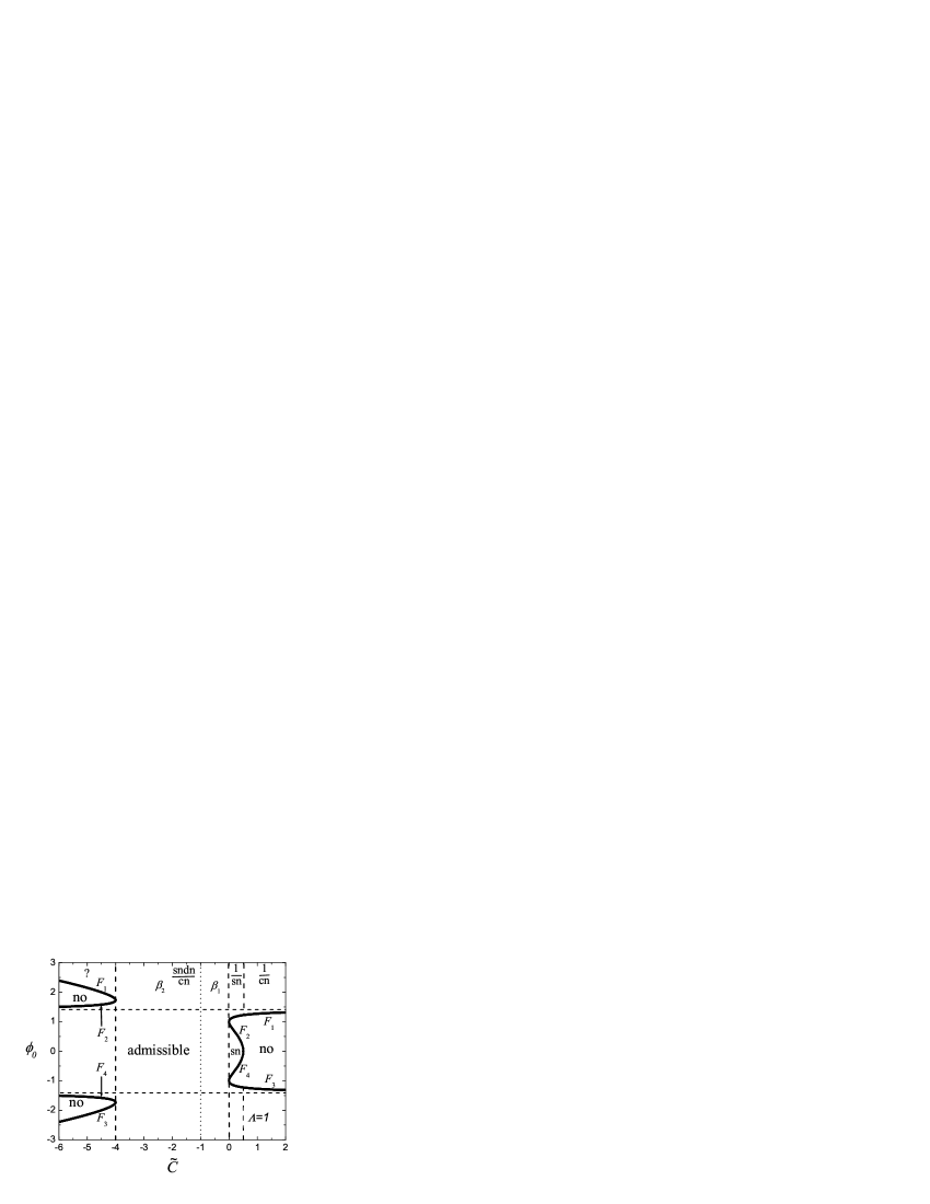
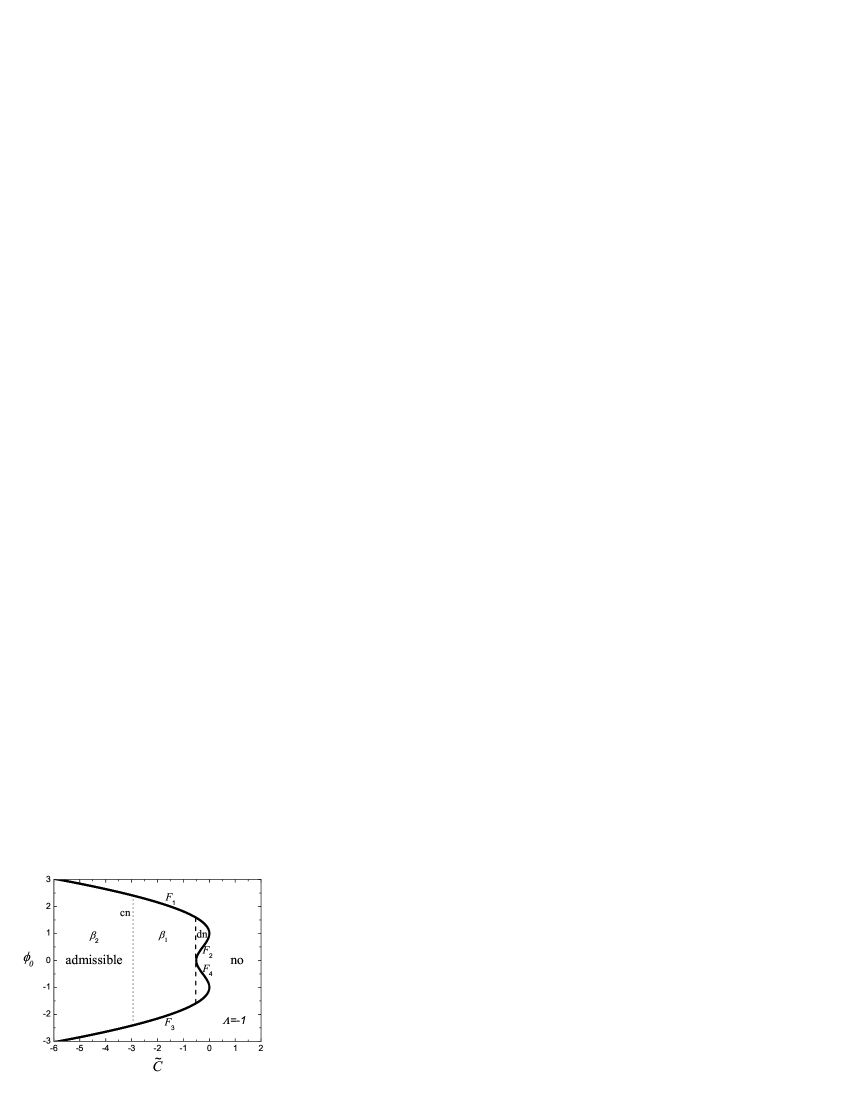
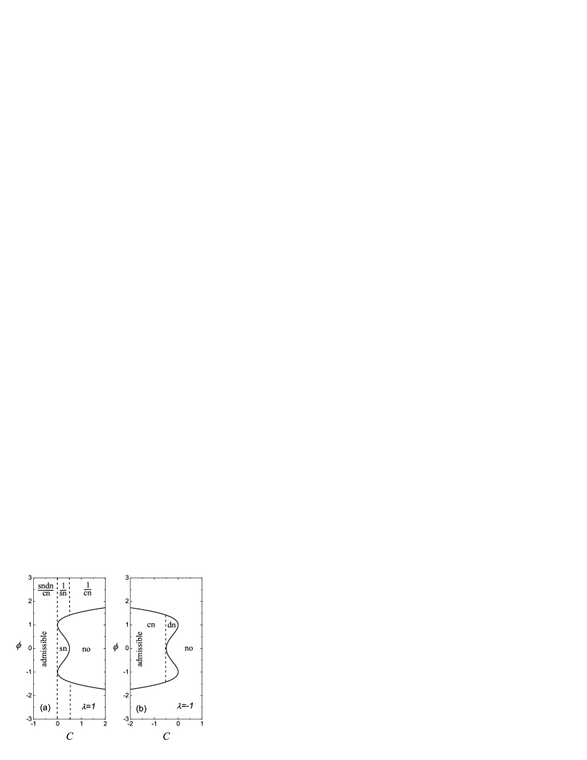
The admissible regions for the values of of the nonlinear map Eq. (40) are shown in Fig. 2 for different values of at . The corresponding result for is presented in Fig. 3. These graphs present a road map for constructing the various possible solutions of the above models.
The symmetry of Eq. (32) suggests that the topology of the admissible regions is such that once started from an admissible value of , one cannot leave the admissible region iterating Eq. (40), so that the static solution will surely be constructed for the whole chain. This is so because Eq. (40) serves for calculating both back and forth points of the map, and if one is admissible, the other one is also admissible.
Equation (40) possesses two roots, which means that for an admissible initial condition one can construct two different solutions, e.g., a kink and an antikink. When iterating, to keep moving along the same solution, one must take different from [if the roots of Eq. (40) are different]. Indeed, setting in the three-point static problem, Eq. (36), , we find
| (43) |
Comparing this with Eq. (40), it is readily seen that the equilibrium in the three-point equation in the case of can be achieved only if and the two roots coincide. As mentioned above, the latter requirement is equivalent to the condition that is on the border of the admissible region.
As it can be deduced from Eq. (41), the topology of the admissible regions presented in Fig. 2 and Fig. 3 does not significantly change among different but positive and among different but negative values of respectively; of course, one has to exclude the particular case of and also the continuum limit (see Sec. VIII). Here we will not discuss in detail the case of extremely high discreteness , even though the analysis of this case does not present any additional difficulties.
To summarize, inside the admissible region, (shown in Figs. 2 and 3), the nonlinear map of Eq. (40) generates static solutions to the MC model of Eq. (36) and to the EC model of Eq. (37).
IV.2 Jacobi elliptic function solutions
Static solutions to the discrete PNb-free models of Eq. (36) and Eq. (37) have been reported Saxena in the form of the Jacobi elliptic functions, and SpecialFunctions . Below, we will derive such solutions.
The general form of the solutions is
| (44) |
where is the modulus of the Jacobi elliptic functions, and are the parameters of the solution, and is the arbitrary initial position. Finally the integers specify a particular form of the solution.
In the limit of , Eq. (44) reduces to the hyperbolic function form
| (45) |
and, in the limit of , to the trigonometric function form
| (46) |
Substituting the ansatz Eq. (44) into Eq. (32) and equalizing the coefficients in front of similar terms we find that it can be satisfied for a limited number of combinations of integer powers . Solving the equations for the coefficients we relate the parameters of the solution Eq. (44), and , to and and also find the relation between , that enters Eq. (32), and .
For some of the sets , e.g., for and for , we obtain imaginary amplitude in the whole range of parameters.
Essentially different, real amplitude solutions described by Eq. (44), have the following form and are characterized by the following parameters:
The solution, ,
| (47) |
The solution, ,
| (48) |
The solution, ,
| (49) |
The solution, ,
| (50) |
The solution, ,
| (51) |
The solution, ,
| (52) |
It is worth making the following remarks:
The solutions should be interpreted in the following form. For a given , one can find by solving the first equation in Eqs. (47-52), and then from the second one. Substituting these values in Eq. (44) results in the static solutions of the original discrete model.
The expressions for in Eqs. (47-52) link the elliptic Jacobi function solutions and the solution in the form of the nonlinear map, Eq. (40). As for the other free parameter of the solutions Eq. (47-52), the arbitrary shift , its counterpart in the nonlinear map, Eq. (40), is effectively the initial value .
The solutions of Eqs. (47-52) can be expressed in a number of other forms using the well-known identities for the Jacobi elliptic functions SpecialFunctions . For example, shifting the argument by a quarter period, one can transform the solution to the form of , or, applying the ascending Landen transformation, to the form of . Mathematically, these three expressions look as different members of Eq. (44), but physically they are indistinguishable.
V Analysis of static solutions
In what follows, we analyze the static solutions derivable from Eq. (40) discussing their relation to Eqs. (47)-(52). Since the topology of the admissible regions is different for positive and negative , these two cases are studied separately.
V.1 case.
In the solution, Eq. (47), when the elliptic modulus increases from its smallest value to its largest value , the amplitude increases from to , since [see Eq. (41) and Eq. (42)]. As a result, the parameter monotonically decreases from to . Thus, the solution is defined in the portion of the -plane, and (see Fig. 2).
The solution, Eq. (50), is defined for , and it is complementary to the solution since it is also valid for , but for (see Fig. 2).
The solution, Eq. (52), is defined for unlimited in the range (see Fig. 2). This solution is only valid for , where, for fixed , is an increasing function of and . For the first expression in Eq. (52) does not have solutions for . For , the equation has two roots, . For the limiting value, , one can find the corresponding amplitude from the second expression of Eq. (52), and then , from the last expression. For the case of presented in Fig. 2, we find and .
It should be noticed that we have not found a solution of the form of Eq. (44) valid in the range of (portion marked with the question mark in Fig. 2). It is likely that static solutions in this range cannot be expressed in terms of the Jacobi elliptic functions because they do not survive in the continuum limit (see Sec. VIII). However, the solution can easily be constructed from the nonlinear map in Eq. (40).
Let us now discuss further several particular examples of the above solutions. First of all, in the limit [see Eq. (45)], the solution, Eq. (47), reduces to the kink solution Saxena ,
| (53) |
while the solution, Eq. (50), to the solution called hereafter the “inverted” kink,
| (54) |
In Eqs. (53) and (54), is the (arbitrary) position of the solution and .
This limiting case corresponds to , for which a heteroclinic connection is possible between the fixed points and (see Fig. 2), giving rise to the kink or the inverted kink. In this case, Eq. (40) assumes the following simple form
| (55) |
where one can choose either the upper or the lower signs. The kink, Eq. (53), and the inverted kink, Eq. (54), can be derived from Eq. (55) taking initial values from and , respectively.
In Fig. 4 we show (a) the kink and (b) the inverted kink solutions taking and , respectively, for .


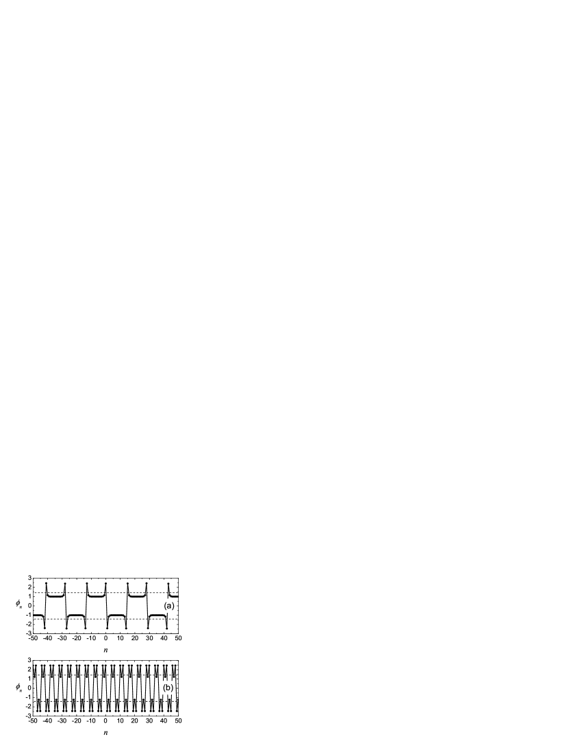
In Fig. 5, and for , we present two examples of solutions for positive and negative close to . In particular, for , taking initial value , we obtain from the map of Eq. (40) the solution presented in panel (a). In fact, it is the solution close to the hyperbolic function limit having the form of a periodic chain of kinks and anti-kinks. On the other hand, for and , we obtain from the map of Eq. (40) the solution shown in panel (b). This is the solution close to the hyperbolic function limit and has a form of a chain of kinks and inverted anti-kinks.
In Fig. 6, and for , we present the solution, Eq. (50), (a) close to the hyperbolic and (b) at the trigonometric limits. The solution shown in panel (a) is a chain of inverted kinks and inverted anti-kinks. These solutions are obtained from the nonlinear map Eq. (40) setting , for (a), and , for (b).
In summary, we have shown that the well-established (hyperbolic and elliptic function) solutions of the model correspond to a very narrow region of the two-parameter () admissible space. A natural question is what is the typical profile outcome stemming from the use of other pairs of and in Eq. (40). Generically, upon testing the different regions of the admissible regime we have observed that arbitrary choices may lead to seemingly erratic solutions with very large amplitudes. A different sign choice in the right hand side of Eq. (40) may, however, lead to a periodically locked tail structure. A simple example of such a solution is given below.
V.2 case.
Let us first start from the latter: When increases from to in Eq. (49), the parameter decreases monotonically from to , i.e., this solution is defined in the “dn” portion of Fig. 3.
On the other hand, the solution of Eq. (48) is only valid for , where is an increasing function of and . For the second expression of Eq. (48) does not have solutions for . For , the equation has two roots, . For the limiting value, , one can find the corresponding amplitude from the second expression of Eq. (48) and then from the last expression. When increases from to in Eq. (48), the parameter of the nonlinear map Eq. (40) corresponding to the root () increases from (decreases from ) to (to ). Thus, the solution occupies the rest of the admissible region for the case of (see Fig. 3). In the case of presented in Fig. 3, we find and .
Both and solutions, in the limit (), reduce to a homoclinic to pulse solution (see also Figs. 1 and 3 where this possibility is illustrated). This solution has the form:
| (56) |
where
| (57) |
This is illustrated by Fig. 7 where, taking , we show the solution obtained from the map Eq. (40) at (a) ( solution) and (b) ( solution), for initial value of . The figure clearly illustrates the two limits (to the left and to the right of ) and their correspondence to pairs of pulse–pulse solutions and ones of pulse–anti-pulse solutions, as one enters the two different regimes “dn” and “cn” of Fig. 3.
V.3 Solutions with
Solutions of this special form can be expressed as with constant and . For the sake of simplicity, we set and substitute the ansatz into Eq. (36) or Eq. (37) to find the zigzag solution
| (58) |
To obtain this solution from the map Eq. (40), one has to set , which is the general condition for getting . Substituting here from Eq. (58), we get . For the case of presented in Fig. 2, we have .
The zigzag solution is an exceptional one, as for any . However, as shown above, this is only possible when Eq. (40) has multiple roots, which means that the two-point static problem, Eq. (32), is factorized. This solution does not have a counterpart in the continuum limit.

VI Linear stability
The static solutions of the discrete models Eq. (36) and Eq. (37) are exactly the same, but the dynamical properties of the two models are different. As the corresponding stability analysis takes into account the dynamical form of each model, it will be carried out separately for each of the two.
Let us first consider the MC model of Eq. (36). Introducing the ansatz (where is an equilibrium solution and is a small perturbation), we linearize Eq. (36) with respect to and obtain the following equation:
| (59) |
For the small-amplitude phonons, , with frequency and wave number , around the uniform steady states (), Eq. (59) is reduced to the following dispersion relation:
| (60) |
while the spectrum of the vacuum solution for , , is
| (61) |
For an arbitrary stationary solution , stability is inferred in the MC model if the eigenvalue problem obtained from Eq. (59) by replacing with has only non-negative solutions . Recalling that the MC model is a non-Hamiltonian one, the resulting eigenvalue problem is a non-self-adjoint one involving a non-symmetric matrix.
Similarly, we obtain analogous expressions for the EC model of Eq. (37). The linearized equation reads
| (62) | |||||
and the corresponding dispersion relation for the linear phonon modes around has the form:
| (63) |
while that of vacuum solution (for ) is
| (64) |
The stationary solution is stable in the EC model of Eq. (37) if the self-adjoint eigenvalue problem obtained from Eq. (62) by replacing with has only non-negative solutions .
We note that all stable and unstable static solutions of the MC and the EC models, except for the zigzag solution Eq. (58), possess a zero-frequency mode. This is a consequence of the effective translational invariance of the discrete PNb-free models; this is related also to the freedom of selecting the free parameter in the corresponding solution expressions.
Our aim here is not to study the whole bunch of solutions in the whole range of parameters, but rather to demonstrate the existence of stable solutions and also provide some examples where solutions, being stable in one model, may be unstable in another. The results of stability analysis for some characteristic solutions are summarized in Table 1.
First, we consider the kink and inverted kink solutions given in Eq. (53) and Eq. (54) respectively: In a numerical experiment, these solutions were placed in the middle of a chain of particles with clamped boundary conditions. We have found that for the chosen set of parameters, the kink is stable in both MC and EC models, while the inverted kink is stable in the EC and unstable in the MC model.
In Fig. 8 we show the spectra of the kink and the inverted kink for their different positions with respect to the lattice, . In the figure, the horizontal lines show the borders of the phonon band of the vacuum and the dots show the frequencies of the kink’s internal modes lying outside of the band. In all cases, the spectra are shown as functions of , even though, admittedly, the kink in the MC model presented in (a) demonstrates very weak sensitivity of its spectrum to variations of .
Let us now consider the periodic solutions depicted in Fig. 5(b) () and in Fig. 6(a) (). For these classes of solutions we used periodic boundary conditions and the length of the lattice was commensurate with the period of the solutions containing a number of periods. Close to the hyperbolic function limit, these solutions are stable in the EC model but unstable in the MC model, following the stability of the building blocks (inverted kinks) associated with these structures. On the other hand, the solution becomes unstable in both models at the trigonometric limit depicted in Fig. 6(b). Nonetheless, we find it remarkable that some of these “apparently non-smooth” solutions (or maybe more correctly, solutions apparently containing a non-smooth continuum limit) may be potentially stable in the discrete setting. It would be wortwhile to analyze the stability of such structures in more detail and as a function of their elliptic modulus .
Next, we consider the zigzag solution, Eq. (58), which exists for . It can be shown that this solution can be stable in the EC model: Indeed, substituting Eq. (58) into the relevant eigenvalue problem, we obtain the dispersion relation for the linear phonon modes, . The solution is stable when are non-negative, i.e., when . Combining this with the existence condition we find that the zigzag solution exists and it is stable in the EC model for . Note that this exceptional solution does not possess the zero frequency mode, as it can be seen from the above dispersion relation. The amplitude of the solution, , is always greater than 1. The zigzag solution is always unstable in the MC model, a result that can similarly be demonstrated.

The , , and solutions close to the hyperbolic limit were found to be generically unstable in both the MC and EC models. The instability of the pulse solution of Eq. (56) can be analytically justified in the present setting. It can be easily inferred from the invariance of the solution with respect to that the eigenvector leading to the zero eigenvalue of Fig. 8 is proportional to (where is the pulse solution profile). This is an anti-symmetric eigenvector, given the pulse’s symmetric (around its center) nature. But then, from Sturm-Liouville theory for discrete operators levy , there should be an eigenvalue such that with a symmetric (i.e., even) eigenvector, resulting in the instability of the relevant pulse solution. Our numerical simulations fully support this conclusion. The pulse solution was constructed by iterating Eq. (40) for , , and , or directly from Eq. (56). We found that for the pulse solution is unstable in both models and over a wide range of the discreteness parameter , including the case of rather small . We have also confirmed that the instability mode is similar to the pulse profile (i.e., of even parity).
Both the cn and dn solutions (see, e.g., Fig. 7) are also found to be unstable for the different parameter values that we have used in both the MC and EC models. This is rather natural to expect given that their “building blocks”, namely the pulse-like solutions are each unstable (hence their concatenation will only add to the unstable eigendirections).
Finally, as far as the sn solutions are concerned, two basic instability modes were revealed. One resembles the instability of the pulse solution, when the whole structure, being waved around the top of the background potential, tends to slide down to one of the potential wells. The other instability modes can be understood if one regards the sn solution as a set of alternating kinks and anti-kinks [see Fig. 5(a)] interacting with each other by means of overlapping tails. Such a system is unstable because the kinks tend to annihilate with the anti-kinks.
It is interesting to note that these stability results suggest a disparity with the earlier numerical findings of Saxena where the pulse-like solution was generically reported to be stable and analogous statements were made for the cn- and dn-type solutions.
At this point, it is worth discussing a connection with NLS-type models mentioned in the introduction. In the case of such models, the aforementioned unstable eigendirection (with an eigenvector similar in profile to the pulse itself) is “prohibited” by the additional conservation law of the norm, resulting in a separate neutral eigendirection with zero eigenfrequency. As a consequence, it is an interesting twist that the instability reported for such pulse-like solutions in scalar models would be absent in their discrete NLS counterparts.
| Solution | MC model, | EC model, |
|---|---|---|
| Eq. (36) | Eq. (37) | |
| kink, Eq. (53) | stable | stable |
| inverted kink, | unstable | stable |
| Eq. (54) | ||
| pulse, Eq. (56) | unstable | unstable |
| sn cn, dn | unstable | unstable |
| close to hyper- | ||
| bolic limit | ||
| sndn/cn, 1/sn | unstable | stable |
| close to hyper- | ||
| bolic limit |
VII Slow kink dynamics
In JPhysA , we have compared the spectra and the long-term dynamics of the kinks in the two PNb-free models, Eq. (36) and Eq. (37), with that of the classical discrete model, Eq. (30) (see Fig. 1 of that paper). The case of very small kink velocities was not studied there. Here we would like to focus on this case to demonstrate the qualitatively different behavior for slowly moving kinks in the PNb-free and classical models.
To boost the kink in the PNb-free models Eq. (36) and Eq. (37) we used the following dynamical solution corresponding to the multiple eigenvalue , , where is a static kink solution, is the normalized translational eigenmode and is the amplitude playing the role of kink velocity. This construction yields a more accurate approximate solution for very small when linearized equations Eq. (59) and Eq. (62) are accurate. Increasing leads to a decrease in the accuracy of the dynamical solution used for boosting. On the other hand, we note in passing that there are techniques developed recently for Klein-Gordon aigner ; oxt1 and even nonlinear Schrödinger lattices preprint that also allow the construction of finite speed, numerically exact travelling solutions in these classes of models.
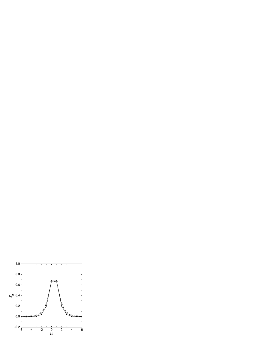
In Fig. 9 we present the lowest frequency normalized eigenmodes for the inter-site kinks in the three models, for the case of , (). Both PNb-free models, Eq. (36) and Eq. (37), have the same translational eigenmodes with , shown by dots connected with solid lines. One can show by straightforward algebra that the PNb-free model modified by a non-vanishing multiplier as described in Sec. II.4 has the same translational eigenmode as the original model. Assuming that the two models are respectively:
| (65) | |||||
| (66) |
where the function , then the steady state solutions will satisfy , for all , while the corresponding linearization equations (using ) are respectively of the form
| (67) | |||||
| (68) |
Hence, when solving the corresponding eigenvalue problem (again substituting by ), for , the eigenvalue problems become identical, both satisfying
| (69) |
hence the coincidence of the corresponding eigenvectors. We are extremely grateful to an anonymous referee for this remark and its proof. We do note, in passing, also that while this justifies the coincidence of the zero eigenfrequency modes of the PNb-free models in Fig. 9, it is also in tune with the results of Fig. 8 for nonzero eigenfrequencies . The latter are not identical between the different models, as indicated by the left and middle panels of that figure. This is due to the differences between the corresponding eigenvalue problems of Eqs. (67) and (68), when .
For the classical model, Eq. (30), the lowest-frequency mode has , and it is shown in Fig. 9 by open circles and dashed lines. Actually, this mode is not a translational mode (since, strictly speaking, there is no translational invariance) but we use it to boost the kink. One can say that this will become the translational mode for this model in the continuum limit.
We define the kink center of mass as
| (70) |
The evolution of the kink coordinates is shown in Fig. 10. Kinks were boosted with two different amplitudes of the normalized lowest-frequency eigenmodes, and . Results for the PNb-free models practically coincide, as depicted by the dashed and solid lines for the MC and EC models, respectively. It is readily seen that kinks in the PNb-free lattices propagate with roughly constant velocities.
The oscillatory trajectories in Fig. 10 correspond to the kink in the classical discrete model. The faster kink, boosted with , propagates along the lattice but its velocity gradually decreases. The kinetic energy of the translational motion is partly lost to the excitation of the kink internal mode with , lying below the phonon frequency band. Higher harmonics of this mode interact with the phonon spectrum producing radiation, which also slows the kink down. An even more dramatic difference is observed for the slower kinks, boosted with . Here, the classical kink cannot overcome the PN barrier and can not propagate, oscillating near the stable inter-site configuration. On the other hand, the kinks in the PNb-free models are not trapped by the lattice and propagate due to the absence of the PN barrier. Alternatively, one can say that such waveforms can be accelerated by arbitrarily small external fields.

VIII Solutions for continuum field
In the continuum limit, , the borders of the admissible region, Eq. (41), become
| (71) |
In Fig. 11 we plot the admissible regions for (a) and (b) . The topology of the admissible regions for the field is simpler than the one pertaining to the discrete models. In the continuum limit there exists a sole inadmissible region for both cases , while three inadmissible regions exist for the discrete models in the case . One more simplification is that the domains of the and solutions do not split into two parts since the smaller root disappears in the continuum limit. Particularly we note that the region marked with the question mark in Fig. 2, , disappears in the continuum limit. That might be the reason why we failed to find a Jacobi elliptic function expression for the discrete static solutions in this case.
Static solutions Eqs. (47-52) obtained for the discrete models have their continuum counterparts as the traveling solutions to the field, Eq. (29). The general form of the solutions is
| (72) |
where is the modulus of the Jacobi elliptic functions, and are the parameters of the solution, is the arbitrary initial position and is the velocity of the solution. The integers once again specify the particular form of the solution.
Continuum analogues of Eqs. (47)-(52) have the following form and are characterized by the following parameters:
The solution, ,
| (73) |
The solution, ,
| (74) |
The solution, ,
| (75) |
The solution, ,
| (76) |
The solution, ,
| (77) |
The solution, ,
| (78) |
The above six solutions can be rewritten in a great variety of forms using the properties of the Jacobi elliptic functions SpecialFunctions . However, we believe that they may constitute the full list of physically different solutions to the continuum equation since they fill the whole two-parameter space, , obtained as the continuum limit of corresponding space of the discrete models.
All solutions are conveniently parameterized by a single parameter for , and for , as it is presented in Fig. 11.
IX Conclusions
In the present paper we have shown that the reduction of the static problem of a discrete Klein-Gordon (and by extension of the standing wave problem of a discrete NLS) equation to a two-point problem is a powerful tool for obtaining all possible static solutions of the corresponding model. We have applied this general idea to a momentum conserving PhysicaD and an energy conserving Saxena discretization of the model analyzing the full two-parameter plane of solutions and giving a natural parametrization for it. In particular, we have examined the admissible regions of the field value at a given point and of the constant entering the two-point function pertinent to the model. We have specifically illustrated how to use different choices of these two parameters to obtain not only the well-known hyperbolic function solutions and the established elliptic function solutions, but also novel classes of solutions including the inverted (non-monotonic) kink solutions presented herein and multi-kink generalizations thereof. We performed such computations both for the attractive (focusing) and for the repulsive (defocusing) types of nonlinearity.
The presented methodology has the significant advantage over earlier work that by introducing the integration constant in the discretization of the first integral of the static part of the PDE, it allows one to construct the full family of the static solutions of the corresponding model. Earlier work had implicitly set this additional free parameter to ; this choice was sufficient for obtaining the important hyperbolic function solutions, but the present formalism systematically illustrates how to generalize the latter.
We have also derived the continuum analogues of the discrete solutions and found that they fill the whole space of parameters obtained in the limit of from the parameter space of the discrete models.
In addition, we have examined some of the key stability features of the solutions obtained in the various models, illustrating the different stability properties of the models considered herein (even if their static solutions are identical). We have obtained interesting stability properties, including, e.g., the counter-intuitive stability of the inverted kink and of some of its periodic generalizations for the EC model.
The present study generates a variety of interesting questions. For instance, it would be relevant to examine whether the solutions presented herein (including the inverted ones) have counterparts in the “standard” discrete model and to analyze their respective stability. It would also be relevant to examine how the stability (and existence –since some of them may not survive the continuum limit–) of such solutions depend on the lattice spacing . Finally, these and related (e.g. stability) questions in the context of discrete NLS lattices (see DNLSE1 ; DNLSE2 ; DEPelinovsky ) would also be equally or even more (given the multitude of relevant applications of the latter model) interesting to answer. Such studies are currently in progress and will be reported elsewhere.
Acknowledgements
The authors would like to thank D. E. Pelinovsky for a number of stimulating and insightful discussions. We are also grateful to an anonymous referee for offering a proof that the MC and EC models have the same translational eigenmodes. PGK gratefully acknowledges support from NSF-DMS-0204585, NSF-DMS-0505663 and NSF-CAREER.
References
- (1) O. M. Braun and Y. S. Kivshar, The Frenkel-Kontorova Model: Concepts, Methods, and Applications (Springer, Berlin, 2004).
- (2) A. Scott, Nonlinear Science: Emergence and Dynamics of Coherent Structures (Oxford Univ. Press, Oxford, 2003).
- (3) M. Toda, Theory of Nonlinear Lattices (Springer-Verlag, Berlin, 1981).
- (4) M. J. Ablowitz and J. F. Ladik, J. Math. Phys. 16, 598 (1975); M. J. Ablowitz and J. F. Ladik, J. Math. Phys. 17, 1011 (1976).
- (5) S. J. Orfanidis, Phys. Rev. D 18, 3828 (1978).
- (6) J. P. Hirth and J. Lothe, Theory of Dislocations (Krieger Publishing, Malabar, Florida, 1992).
- (7) T. I. Belova and A. E. Kudryavtsev, Phys. Usp. 40, 359 (1997).
- (8) A. A. Aigner, A. R. Champneys and V. M. Rothos, Physica D 186, 148 (2003).
- (9) J. M. Speight, and R. S. Ward, Nonlinearity 7, 475 (1994); J. M. Speight, Nonlinearity 10, 1615 (1997); J. M. Speight, Nonlinearity 12, 1373 (1999).
- (10) E. B. Bogomol’nyi, J. Nucl. Phys. 24, 449 (1976).
- (11) P. G. Kevrekidis, Physica D 183, 68 (2003).
- (12) S. V. Dmitriev, P. G. Kevrekidis, and N. Yoshikawa, J. Phys. A 39, 7217 (2006).
- (13) I. V. Barashenkov, O. F. Oxtoby, and D. E. Pelinovsky, Phys. Rev. E 72, 35602R (2005).
- (14) S. Aubry, J. Chem. Phys. 64, 3392 (1976).
- (15) S. V. Dmitriev, P. G. Kevrekidis, and N. Yoshikawa, J. Phys. A 38, 7617 (2005).
- (16) F. Cooper, A. Khare, B. Mihaila, and A. Saxena, Phys. Rev. E 72, 36605 (2005).
- (17) J. M. Speight and Y. Zolotaryuk, Nonlinearity 19, 1365 (2006).
- (18) M. J. Ablowitz, B. Prinari and A. D. Trubatch, Discrete and continuous nonlinear Schrödinger systems, (Cambridge Univ. Press, Cambridge, 2004).
- (19) H. Levy and F. Lessman, Finite Difference Equations (Dover, New York, 1992).
- (20) Handbook of mathematical functions, edited by M. Abramowitz and I. A. Stegun (U. S. GPO, Washington, D.C., 1964).
- (21) O.F. Oxtoby, D.E. Pelinovsky and I.V. Barashenkov, Nonlinearity 19, 217 (2006).
- (22) see e.g. the recent preprint: T.R.O. Melvin, A.R. Champneys, P.G. Kevrekidis and J. Cuevas, nlin.PS/0603071.
- (23) P. G. Kevrekidis, S. V. Dmitriev, and A. A. Sukhorukov, Mathematics and Computers in Simulation (in press).
- (24) S.V. Dmitriev, P.G. Kevrekidis, A.A. Sukhorukov, N. Yoshikawa and S. Takeno, Phys. Lett. A 356, 324 (2006) (see also nlin.PS/0603047, with corrected misprints).
- (25) D. E. Pelinovsky, nlin.PS/0603022.