Solutions of Non-Integrable Equations by the Hirota Direct Method

Abstract

We show that we can also apply the Hirota method to some non-integrable equations. For this purpose, we consider the extensions of the Kadomtsev-Petviashvili (KP) and the Boussinesq (Bo) equations. We present several solutions of these equations.

1 Introduction

The Hirota direct method is one of the famous method to construct multi-soliton solutions of integrable nonlinear partial differential equations. Hirota gave the exact solution of the Korteweg-de Vries (KdV) equation for multiple collisions of solitons by using the Hirota direct method in $1971$ [1]. In his successive articles, he dealt also with many other nonlinear evolution equations such as the modified Korteweg-de Vries (mKdV) [2], sine-Gordon (sG) [3], nonlinear Schrödinger (nlS) [4] and Toda lattice (Tl) [5] equations.

The first step of this method is to transform the nonlinear partial differential or difference equation into a quadratic form in dependent variables. The new form of the equation is called ’bilinear form’. In the second step, we write the bilinear form the equation as a polynomial of a special differential operator, Hirota D-operator. This polynomial of D-operator is called ’Hirota bilinear form’. In fact, some equations may not be written in the Hirota bilinear form but perhaps in trilinear or multilinear forms [6]. The last step of the method is using the finite perturbation expansion in the Hirota bilinear form. We analyze the coefficients of the perturbation parameter and its powers separately. Here the information we gain makes us to reach the exact solution of the equation.

The equations having Hirota bilinear form possesses automatically one- and two-soliton solutions. But when we try to construct the three-soliton solutions we come across a very restrictive condition. This condition was used as a powerful tool to search the integrability of the equations by Hietarinta [7]. Hietarinta also used this condition to produce new integrable equations in his articles [8], [9], [10], [11].

Most of the works dealt with the Hirota direct method is about the integrable equations. But in this work, we show that the Hirota direct method also can be used to find exact solutions of some non-integrable nonlinear partial differential equations. For illustration we consider an extension of the Kadomtsev-Petviashvili (KP) equation,

$$(u_{t}-6uu_{x}+u_{xxx})_{x}+3u_{yy}+au_{tt}+bu_{ty}+c\nabla^{2}u=0$$ (1)

where $a$, $b$ and $c$ are constants and $\nabla^{2}u=u_{x_{1}x_{1}}+u_{x_{2}x_{2}}+...+u_{x_{m}x_{m}}$ for $x_{j}$, $j=1,2,...,m$ are independent variables. This extension of the KP equation has bilinear and Hirota bilinear form so the Hirota direct method is applicable. But when we obtain exact solutions, we shall consider the case $c=0$. In this case the equation turns out to be

$$(u_{t}-6uu_{x}+u_{xxx})_{x}+3u_{yy}+au_{tt}+bu_{ty}=0$$ (2)

and we call it as the extended Kadomtsev-Petviashvili (eKP) equation. This equation is integrable if $a=b^{2}/12$. The equation with this condition is equivalent to the KP equation. We find exact solution of this equation by using the Hirota method for all $a$, $b$. Another example to this fact is the extension of the Boussinesq (Bo) equation which is

$$u_{tt}-u_{xx}+3(u^{2})_{xx}-u_{xxxx}+au_{yy}+bu_{ty}+c\nabla^{2}u=0.$$ (3)

Similar to the extension of the KP equation, $a$, $b$ and $c$ are constants. When $c\neq 0$, we can also apply the Hirota method to this equation since it has bilinear and Hirota bilinear form. But again, when we consider the exact solutions, we shall take $c=0$. So we deal with the equation

$$u_{tt}-u_{xx}+3(u^{2})_{xx}-u_{xxxx}+au_{yy}+bu_{ty}=0$$ (4)

which we call the extended Boussinesq (eBo) equation. The eBo equation is integrable if $a=b^{2}/4$. Indeed, under this condition, it is equivalent to the Bo equation. The Hirota method gives the exact solutions of the eBo equation for all $a$, $b$. Before passing to the application of the Hirota direct method, let us see how this method works.

1.1 The Hirota Direct Method

We review the Hirota direct method in four steps by following Hietarinta’s article [12] closely. Let $F[u]=F(u,u_{x},u_{t},...)$ be a nonlinear partial differential equation.

Step $1$: Bilinearization: We transform $F[u]$ to a quadratic form in the dependent variables by a bilinearizing transformation $u=T[f(x,t,...),g(x,t,...)]$. We call this form the bilinear form of $F[u]$. Note that for some equations we may not find such a transformation.

Step $2$: Transformation to the Hirota bilinear form:

Definition 1.1.

Let $S:{\mathbb{C}}^{n}\rightarrow{\mathbb{C}}$ be a space of differentiable functions. Then Hirota D-operator $D:S\times S\rightarrow S$ is defined as

$$[D_{x}^{m_{1}}D_{t}^{m_{2}}...]\{f.g\}=[(\partial_{x}-\partial_{x^{\prime}})^{m_{1}}(\partial_{t}-\partial_{t^{\prime}})^{m_{2}}...]f(x,t,...)\\ \times g(x^{\prime},t^{\prime},...)|_{x^{\prime}=x,t^{\prime}=t,...}$$ (5)

where $m_{i}$, $i=1,2,...$ are positive integers and $x,t,...$ are independent variables.

By using some sort of combination of Hirota D-operator, we try to write the bilinear form of $F[u]$ as a polynomial of D-operator, say $P(D)$. Let us state some propositions and corollaries on $P(D)$ [12].

Proposition 1.2.

Let $P(D)$ act on two differentiable functions $f(x,t,...)$ and $g(x,t,...)$. Then we have

$$P(D)\{f.g\}=P(-D)\{g.f\}.$$ (6)

Corollary 1.3.

Let $P(D)$ act on two differentiable functions $f(x,t,...)$ and $g=1$, then we have

$$P(D)\{f.1\}=P(\partial)f\quad,\quad P(D)\{1.f\}=P(-\partial)f.$$ (7)

Proposition 1.4.

Let P(D) act on two exponential functions $e^{\theta_{1}}$ and $e^{\theta_{2}}$ where $\theta_{i}=k_{i}x+w_{i}t+...+\alpha_{i}$ with $k_{i},w_{i},...,\alpha_{i}$ are constants for $i=1,2$. Then we have

$$P(D)\{e^{\theta_{1}}.e^{\theta_{2}}\}=P(k_{1}-k_{2},...,\alpha_{1}-\alpha_{2})e^{\theta_{1}+\theta_{2}}.$$ (8)

For a shorter notation, we use $P(p_{1}-p_{2})$ instead of $P(k_{1}-k_{2},...,\alpha_{1}-\alpha_{2})$.

Corollary 1.5.

If we have $P(D)\{a.a\}=0$ where $a$ is any nonzero constant then we have $P(0,0,...)=0$.

Definition 1.6.

We say that a nonlinear partial differential equation can be written in Hirota bilinear form if it is equivalent to

$$\sum_{\alpha,\beta=1}^{m}P_{\alpha\beta}^{\eta}(D)f^{\alpha}.f^{\beta}=0,\quad\eta=1,...,r$$ (9)

for some m,r and linear operators $P_{\alpha\beta}^{\eta}(D)$. The $f^{i}$’s are new dependent variables.

Remark 1.7.

There is no systematic way to write a nonlinear partial differential equation in Hirota bilinear form.

Remark 1.8.

For some nonlinear partial differential equations we may need more than one Hirota bilinear equation.

Step $3$: Application of the Hirota perturbation: We substitute the finite perturbation expansions of the differentiable functions $f(x,t,...)$ and $g(x,t,...)$ which are

$$f(x,t,...)=f_{0}+\sum_{m=1}^{N}\varepsilon^{m}f_{m}(x,t,...)\quad,\quad g(x,t,...)=g_{0}+\sum_{m=1}^{N}\varepsilon^{m}g_{m}(x,t,...)$$ (10)

into the Hirota bilinear form. Here $f_{0}$, $g_{0}$ are constants with the condition $(f_{0},g_{0})\neq(0,0)$ to avoid the trivial solution. For the sake of applicability of the method we take the functions $f_{m}$ and $g_{m}$, $m=1,...,N$ as exponential functions. $\varepsilon$ is a constant called the perturbation parameter. For instance for $N=2$, we take

$$f=f_{0}+\varepsilon f_{1}+\varepsilon^{2}f_{2}\quad,\quad g=g_{0}+\varepsilon g_{1}+\varepsilon^{2}g_{2}$$ (11)

where $f_{1}=e^{\theta_{1}}+e^{\theta_{2}}$ for $\theta_{i}=k_{i}x+\omega_{i}t+...+\alpha_{i}$, $i=1,2$. We decide what the other terms of the functions $f$ and $g$ in the process of the method.

Step $4$: Examination of the coefficients of the perturbation parameter $\varepsilon$: We make the coefficients of the perturbation parameter $\varepsilon$ and its powers appeared in the Hirota perturbation to vanish. From these coefficients we obtain the functions $f(x,t,...)$ and $g(x,t,...)$. Hence by using them in the bilinearizing transformation $u=T[f(x,t,...),g(x,t,...)]$, we find the exact solution of $F[u]$.

2 Applications of the Hirota Direct Method

2.1 The Extended Kadomtsev-Petviashvili (EKP)
Equation

The extended Kadomtsev-Pethviashvili (eKP) equation is given by

$$(u_{t}-6uu_{x}+u_{xxx})_{x}+3u_{yy}+au_{tt}+bu_{ty}+c\nabla^{2}u=0$$ (12)

which is constructed by adding the terms $au_{tt}$, $bu_{ty}$ and $\nabla^{2}u=u_{x_{1}x_{1}}+u_{x_{2}x_{2}}+...+u_{x_{m}x_{m}}$ multiplied by $c$ to the Kadomtsev-Petviashvili (KP) equation where $a$, $b$ and $c$ are constants and $x_{j}$, $j=1,2,...,m$ are independent variables. Now let us apply the Hirota direct method to the eKP equation.

Step $1$. Bilinearization: We use the bilinearizing transformation

$$u(x,t,y)=-2\partial_{x}^{2}\log f$$ (13)

so the bilinear form of eKP is

$$f_{tx}f-f_{t}f_{x}+f_{xxxx}f-4f_{x}f_{xxx}+3f_{xx}^{2}+3f_{yy}f-3f_{y}^{2}\\ +aff_{tt}-af_{t}^{2}+bf_{ty}f-bf_{t}f_{y}+c\sum_{j=1}^{m}(f_{x_{j}x_{j}}f-f_{x_{j}}^{2})=0.$$ (14)

Step $2$. Transformation to the Hirota bilinear form: The Hirota bilinear form of eKP is

$$P(D)\{f.f\}=(D_{t}D_{x}+D_{x}^{4}+3D_{y}^{2}+aD_{t}^{2}+bD_{t}D_{y}+c\sum_{j=1}^{m}D_{x_{j}}^{2})\{f.f\}=0.$$ (15)

Step $3$. Application of the Hirota perturbation: Insert $f=1+\sum_{n=1}^{N}\varepsilon^{n}f_{n}$ into the equation (15) so we have

$$P(D)\{f.f\}=P(D)\{1.1\}+\varepsilon P(D)\{f_{1}.1+1.f_{1}\}\\ +...+\varepsilon^{2N}P(D)\{f_{N}.f_{N}\}=0.$$ (16)

Step $4$: Examination of the coefficients of the perturbation parameter $\varepsilon$: We make the coefficients of $\varepsilon^{m}$, $m=1,2,...,N$ appeared in 16 to vanish. Here we shall consider only the case $N=3$ and $N=4$. Note that since eKP is not integrable except if $a=b^{2}/12$, we call the solutions obtained using the Hirota method as the $N$-Hirota solution of eKP.

2.1.1 $N=3$, Three-Hirota Solution of EKP

Here we apply the Hirota direct method by using the anzats which is used to construct three-soliton solutions. We take $f=1+\varepsilon f_{1}+\varepsilon^{2}f_{2}+\varepsilon^{3}f_{3}$ where $f_{1}=e^{\theta_{1}}+e^{\theta_{2}}+e^{\theta_{3}}$ with $\theta_{i}=k_{i}x+\omega_{i}t+l_{i}y+\sum_{j=1}^{m}r_{ij}x_{j}+\alpha_{i}$ for $i=1,2,3$ and insert it into (16). The coefficient of $\varepsilon^{0}$ is identically zero since

$$P(D)\{1.1\}=0.$$ (17)

By the coefficient of $\varepsilon^{1}$

$$P(D)\{1.f_{1}+f_{1}.1\}=2P(\partial)\{e^{\theta_{1}}+e^{\theta_{2}}+e^{\theta_{3}}\}=0$$ (18)

we have the relation

$$P(p_{i})=k_{i}\omega_{i}+k_{i}^{4}+3l_{i}^{2}+a\omega_{i}^{2}+b\omega_{i}l_{i}+c\sum_{j}^{m}r_{ij}^{2}=0$$ (19)

for $i=1,2,3$. This relation is called as the dispersion relation. Note that when $c$, the coefficient of $\nabla^{2}u$ is not zero, we can apply the Hirota direct method. But for simplicity, we take $c=0$ in the rest of the calculations. In this case $\theta_{i}$ turn out to be $\theta_{i}=k_{i}x+\omega_{i}t+l_{i}y+\alpha_{i}$, $i=1,2,3$. From the coefficient of $\varepsilon^{2}$ we get

$$-P(\partial)f_{2}=\sum_{i<j}^{(3)}[(k_{i}-k_{j})(\omega_{i}-\omega_{j})+(k_{i}-k_{j})^{4}+3(l_{i}-l_{j})^{2}\\ +a(\omega_{i}-\omega_{j})^{2}+b(\omega_{i}-\omega_{j})(l_{i}-l_{j})]e^{\theta_{i}+\theta_{j}}$$ (20)

where $(3)$ indicates the summation of all possible combinations of the three elements with $i<j$. Thus $f_{2}$ should be of the form

$$f_{2}=A(1,2)e^{{\theta_{1}}+{\theta_{2}}}+A(1,3)e^{{\theta_{1}}+{\theta_{3}}}+A(2,3)e^{{\theta_{2}}+{\theta_{3}}}$$ (21)

to satisfy the equation. We insert $f_{2}$ into the equation (20) so we get $A(i,j)$ as

$$\begin{split}A(i,j)&=-\frac{P(p_{i}-p_{j})}{P(p_{i}+P_{j})}\\ &=\displaystyle\frac{b(\omega_{i}l_{j}+\omega_{j}l_{i})+2a\omega_{i}\omega_{j}+k_{i}(\omega_{j}+4k_{j}^{3})+k_{j}(\omega_{i}+4k_{i}^{3})-6k_{i}^{2}k_{j}^{2}+6l_{i}l_{j}}{b(\omega_{i}l_{j}+\omega_{j}l_{i})+2a\omega_{i}\omega_{j}+k_{i}(\omega_{j}+4k_{j}^{3})+k_{j}(\omega_{i}+4k_{i}^{3})+6k_{i}^{2}k_{j}^{2}+6l_{i}l_{j}}\end{split}$$ (22)

where $i,j=1,2,3$, $i<j$. From the coefficient of $\varepsilon^{3}$ we obtain

$$P(\partial)\{f_{3}\}=-[A(1,2)P(p_{3}-p_{2}-p_{1})+A(1,3)P(p_{2}-p_{1}-p_{3})\\ +A(2,3)P(p_{1}-p_{2}-p_{3})]e^{{\theta_{1}}+{\theta_{2}}+{\theta_{3}}}.$$ (23)

Hence $f_{3}$ is in the form $f_{3}=Be^{{\theta_{1}}+{\theta_{2}}+{\theta_{3}}}$ where $B$ is found as

$$B=\displaystyle-\frac{A(1,2)P(p_{3}-p_{1}-p_{2})+A(1,3)P(p_{2}-p_{1}-p_{3})+A(2,3)P(p_{1}-p_{2}-p_{3})}{P(p_{1}+p_{2}+p_{3})}.$$ (24)

The coefficient of $\varepsilon^{4}$ gives us

$$e^{{2\theta_{1}}+{\theta_{2}}+{\theta_{3}}}[BP(p_{2}+p_{3})+A(1,2)A(1,3)P(p_{2}-p_{3})]\\ +e^{{\theta_{1}}+{2\theta_{2}}+{\theta_{3}}}[BP(p_{1}+p_{3})+A(1,2)A(2,3)P(p_{1}-p_{3})]\\ +e^{{\theta_{1}}+{\theta_{2}}+{2\theta_{3}}}[BP(p_{1}+p_{2})+A(1,3)A(2,3)P(p_{1}-p_{2})]=0$$ (25)

which is satisfied when

$$B=A(1,2)A(1,3)A(2,3).$$ (26)

To be consistent the two expressions (24) and (26) should be equivalent i.e.

$$\begin{split}B=&\displaystyle-\frac{A(1,2)P(p_{3}-p_{1}-p_{2})+A(1,3)P(p_{2}-p_{1}-p_{3})+A(2,3)P(p_{1}-p_{2}-p_{3})}{P(p_{1}+p_{2}+p_{3})}\\ =&A(1,2)A(1,3)A(2,3).\end{split}$$ (27)

The above equivalence is satisfied when the condition

$$\begin{split}&P(p_{1}-p_{2})P(p_{1}-p_{3})P(p_{2}-p_{3})P(p_{1}+p_{2}+p_{3})\\ +&P(p_{1}-p_{2})P(p_{1}+p_{3})P(p_{2}+p_{3})P(p_{3}-p_{1}-p_{2})\\ +&P(p_{1}-p_{3})P(p_{1}+p_{2})P(p_{2}+p_{3})P(p_{2}-p_{1}-p_{3})\\ +&P(p_{2}-p_{3})P(p_{1}+p_{2})P(p_{1}+p_{3})P(p_{1}-p_{2}-p_{3})=0\end{split}$$ (28)

holds. This condition which we call three-Hirota solution condition $(3HC)$ can also be written as

$$\sum_{\sigma_{r}=\pm 1}P(\sigma_{1}p_{1}+\sigma_{2}p_{2}+\sigma_{3}p_{3})P(\sigma_{1}p_{1}-\sigma_{2}p_{2})P(\sigma_{2}p_{2}-\sigma_{3}p_{3})P(\sigma_{1}p_{1}-\sigma_{3}p_{3})=0,$$ (29)

$r=1,2,3$. After some simplifications $(3HC)$ turns out to be

$$\begin{split}&(12a-b^{2})k_{1}^{2}k_{2}^{2}k_{3}^{2}\Big{[}2k_{1}^{2}w_{2}w_{3}l_{2}l_{3}+2k_{2}^{2}w_{1}w_{3}l_{1}l_{3}+2k_{3}^{2}w_{1}w_{2}l_{1}l_{2}\\ &+2k_{2}k_{3}w_{2}w_{3}l_{1}^{2}+2k_{1}k_{3}w_{1}w_{3}l_{2}^{2}+2k_{1}k_{2}w_{1}w_{2}l_{3}^{2}+2k_{2}k_{3}w_{1}^{2}l_{2}l_{3}\\ &+2k_{1}k_{3}w_{2}^{2}l_{1}l_{3}+2k_{1}k_{2}w_{3}^{2}l_{1}l_{2}-2k_{1}k_{3}w_{2}w_{3}l_{1}l_{2}-2k_{1}k_{3}w_{1}w_{2}l_{2}l_{3}\\ &-2k_{1}k_{2}w_{2}w_{3}l_{1}l_{3}-2k_{1}k_{2}w_{1}w_{3}l_{2}l_{3}-2k_{2}k_{3}w_{1}w_{3}l_{1}l_{2}-2k_{2}k_{3}w_{1}w_{2}l_{1}l_{3}\\ &-k_{1}^{2}w_{3}^{2}l_{2}^{2}-k_{1}^{2}w_{2}^{2}l_{3}^{2}-k_{2}^{2}w_{1}^{2}l_{3}^{2}-k_{2}^{2}w_{3}^{2}l_{1}^{2}-k_{3}^{2}w_{2}^{2}l_{1}^{2}-k_{3}^{2}w_{1}^{2}l_{2}^{2}\Big{]}=0.\end{split}$$ (30)

As we see this condition satisfied when $a=b^{2}/12$ or for some relations on $k_{i}$, $w_{i}$ and $l_{i}$ which violate the solitonic property of the solution. The coefficients of $\varepsilon^{5}$ and $\varepsilon^{6}$ vanish trivially. Let us focus on the condition (30). When the relation $a=b^{2}/12$ holds, the eKP equation is integrable. In fact, it is transformable to the KP equation by the transformation

$u^{\prime}=u$, $x^{\prime}=x$, $y^{\prime}=y$, $t^{\prime}=t+\rho y$,

where $\rho=-b/6=\sqrt{a/3}$. If $a\neq b^{2}/12$, eKP is not integrable. In this case, there are other relations which provide (30) satisfied. Some of them are;

Case 1. Any $k_{i}=0$, $i=1,2,3$, the rest are different,

Case 2. $k_{i}=\omega_{i}$, $i=1,2,3$,

Case 3. $k_{i}=l_{i}$, $i=1,2,3$,

Case 4. $\omega_{i}=l_{i}$, $i=1,2,3$.

By using any of these cases, we obtain the exact solutions of eKP.

2.1.2 $N=4$, Four-Hirota Solution of EKP

Here we apply the Hirota direct method by using the anzats which is used to construct four-soliton solutions. We take $f=1+\varepsilon f_{1}+\varepsilon^{2}f_{2}+\varepsilon^{3}f_{3}+\varepsilon^{4}f_{4}$ where $f_{1}=e^{\theta_{1}}+e^{\theta_{2}}+e^{\theta_{3}}+e^{\theta_{4}}$ with $\theta_{i}=k_{i}x+\omega_{i}t+l_{i}y+\alpha_{i}$ for $i=1,2,3,4$ and insert it into (16). We will only consider the coefficients of $\varepsilon^{m}$, $m=1,2,3,4,5$ since the others vanish identically. By the coefficient of $\varepsilon^{1}$

$$P(D)\{1.f_{1}+f_{1}.1\}=2P(\partial)\{e^{\theta_{1}}+e^{\theta_{2}}+e^{\theta_{3}}+e^{\theta_{4}}\}=0$$ (31)

we have the dispersion relation

$$P(p_{i})=k_{i}\omega_{i}+k_{i}^{4}+3l_{i}^{2}+a\omega_{i}^{2}+b\omega_{i}l_{i}=0$$ (32)

for $i=1,2,3,4$. From the coefficient of $\varepsilon^{2}$ we get

$$-P(\partial)f_{2}=P(p_{1}-p_{2})e^{\theta_{1}+\theta_{2}}+P(p_{1}-p_{3})e^{\theta_{1}+\theta_{3}}+P(p_{1}-p_{4})e^{\theta_{1}+\theta_{4}}\\ +P(p_{2}-p_{3})e^{\theta_{2}+\theta_{3}}+P(p_{2}-p_{4})e^{\theta_{2}+\theta_{4}}+P(p_{3}-p_{4})e^{\theta_{3}+\theta_{4}}.$$ (33)

Thus $f_{2}$ should be of the form

$$f_{2}=A(1,2)e^{{\theta_{1}}+{\theta_{2}}}+A(1,3)e^{{\theta_{1}}+{\theta_{3}}}+A(1,4)e^{\theta_{1}+\theta_{4}}\\ +A(2,3)e^{{\theta_{2}}+{\theta_{3}}}+A(2,4)e^{\theta_{2}+\theta_{4}}+A(3,4)e^{\theta_{3}+\theta_{4}},$$ (34)

where $A(i,j)$, $i,j=1,2,3,4$ with $i<j$ are obtained as

$$\begin{split}A(i,j)&=-\frac{P(p_{i}-p_{j})}{P(p_{i}+P_{j})}\\ &=\displaystyle\frac{\beta(\omega_{i}l_{j}+\omega_{j}l_{i})+2\gamma\omega_{i}\omega_{j}+k_{i}(\omega_{j}+4k_{j}^{3})+k_{j}(\omega_{i}+4k_{i}^{3})-6k_{i}^{2}k_{j}^{2}+6l_{i}l_{j}}{\beta(\omega_{i}l_{j}+\omega_{j}l_{i})+2\gamma\omega_{i}\omega_{j}+k_{i}(\omega_{j}+4k_{j}^{3})+k_{j}(\omega_{i}+4k_{i}^{3})+6k_{i}^{2}k_{j}^{2}+6l_{i}l_{j}}.\end{split}$$ (35)

After some simplifications, the coefficient of $\varepsilon^{3}$ gives

$$-P(\partial)f_{3}=\sum_{i<j<m}^{(4)}[A(i,j)P(p_{m}-p_{i}-p_{j})+A(i,m)P(p_{j}-p_{i}-p_{m})\\ +A(j,m)P(p_{i}-p_{j}-p_{m})]e^{\theta_{i}+\theta_{j}+\theta_{m}}$$ (36)

where $(4)$ indicates the summation of all possible combinations of the four elements with $i<j<m$. Hence $f_{3}$ is of the form

$$f_{3}=B(1,2,3)e^{{\theta_{1}}+{\theta_{2}}+{\theta_{3}}}+B(1,2,4)e^{{\theta_{1}}+{\theta_{2}}+{\theta_{4}}}\\ +B(1,3,4)e^{{\theta_{1}}+{\theta_{3}}+{\theta_{4}}}+B(2,3,4)e^{{\theta_{2}}+{\theta_{3}}+{\theta_{4}}}.$$ (37)

We insert $f_{3}$ into (36) and obtain

$$B(i,j,m)=\displaystyle-\frac{A(i,j)P(p_{m}-p_{i}-p_{j})+A(i,m)P(p_{j}-p_{i}-p_{m})+A(j,m)P(p_{i}-p_{j}-p_{m})}{P(p_{i}+p_{j}+p_{m})}$$ (38)

for $i,j,m=1,2,3,4$ with $i<j<m$. From the coefficient of $\varepsilon^{4}$ we have

$$\begin{split}P(D)\{f_{4}.1+f_{3}.f_{1}+f_{2}.f_{2}+f_{1}.f_{3}+1.f_{4}\}&=2P(\partial)f_{4}+2P(D)\{f_{1}.f_{3}\}+P(D)\{f_{2}.f_{2}\}\\ &=0.\end{split}$$ (39)

The simplifications gives us that we should have

$$B(i,j,m)=A(i,j)A(i,m)A(j,m)$$ (40)

for $i,j,m=1,2,3,4$ with $i<j<m$. To have consistency the equations (38) and (40) should be equivalent. This yields the condition

$$\sum_{\sigma_{r}=\pm 1}P(\sigma_{i}p_{i}+\sigma_{j}p_{j}+\sigma_{m}p_{m})P(\sigma_{i}p_{i}-\sigma_{j}p_{j})P(\sigma_{j}p_{j}-\sigma_{m}p_{m})P(\sigma_{i}p_{i}-\sigma_{m}p_{m})=0.$$ (41)

for $i,j,m,r=1,2,3,4$ with $i<j<m$, which turns out to be

$$\begin{split}&(12a-b^{2})k_{i}^{2}k_{j}^{2}k_{m}^{2}\Big{[}2k_{i}^{2}w_{j}w_{m}l_{j}l_{m}+2k_{j}^{2}w_{i}w_{m}l_{i}l_{m}+2k_{m}^{2}w_{i}w_{j}l_{i}l_{j}\\ &+2k_{j}k_{m}w_{j}w_{m}l_{i}^{2}+2k_{i}k_{m}w_{i}w_{m}l_{j}^{2}+2k_{i}k_{j}w_{i}w_{j}l_{m}^{2}+2k_{j}k_{m}w_{i}^{2}l_{j}l_{m}\\ &+2k_{i}k_{m}w_{j}^{2}l_{i}l_{m}+2k_{i}k_{j}w_{m}^{2}l_{i}l_{j}-2k_{i}k_{m}w_{j}w_{m}l_{i}l_{j}-2k_{i}k_{m}w_{i}w_{j}l_{j}l_{m}\\ &-2k_{i}k_{j}w_{j}w_{m}l_{i}l_{m}-2k_{i}k_{j}w_{i}w_{m}l_{j}l_{m}-2k_{j}k_{m}w_{i}w_{m}l_{i}l_{j}-2k_{j}k_{m}w_{i}w_{j}l_{i}l_{m}\\ &-k_{i}^{2}w_{m}^{2}l_{j}^{2}-k_{i}^{2}w_{j}^{2}l_{m}^{2}-k_{j}^{2}w_{i}^{2}l_{m}^{2}-k_{j}^{2}w_{m}^{2}l_{i}^{2}-k_{m}^{2}w_{j}^{2}l_{i}^{2}-k_{m}^{2}w_{i}^{2}l_{j}^{2}\Big{]}=0\end{split}$$ (42)

where $i,j,m=1,2,3,4$, $i<j<m$. Some of the relations except $a=b^{2}/12$ which make this condition satisfied are;

Case 1. Any two of $k_{i}=0$, $i=1,2,3,4$, the rest are different,

Case 2. $k_{i}=\omega_{i}$, $i=1,2,3,4$,

Case 3. $k_{i}=l_{i}$, $i=1,2,3,4$,

Case 4. $\omega_{i}=l_{i}$, $i=1,2,3,4$.

The equation remaining from the coefficient of $\varepsilon^{4}$ is

$$-P(\partial)f_{4}=e^{\theta_{1}+\theta_{2}+\theta_{3}+\theta_{4}}[B_{123}P(p_{4}-p_{1}-p_{2}-p_{3})+B_{124}P(p_{3}-p_{1}-p_{2}-p_{4})]\\ +B_{134}P(p_{2}-p_{1}-p_{3}-p_{4})+B_{234}P(p_{1}-p_{2}-p_{3}-p_{4})+A(1,2)A(3,4)P(p_{1}+p_{2}-p_{3}-p_{4})\\ +A(1,3)A(2,4)P(p_{1}+p_{3}-p_{2}-p_{4})+A(1,4)A(2,3)P(p_{1}+p_{4}-p_{2}-p_{3})]=0.$$ (43)

Thus $f_{4}=Ce^{\theta_{1}+\theta_{2}+\theta_{3}+\theta_{4}}$ where $C$ is obtained as

$$\begin{split}C=-[&A(1,2)A(3,4)P(p_{1}+p_{2}-p_{3}-p_{4})+A(1,3)A(2,4)P(p_{1}+p_{3}-p_{2}-p_{4})\\ +&A(1,4)A(2,3)P(p_{1}+p_{4}-p_{2}-p_{3})+B(1,2,3)P(p_{4}-p_{1}-p_{2}-p_{3})\\ +&B(1,2,4)P(p_{3}-p_{1}-p_{2}-p_{4})+B(1,3,4)P(p_{2}-p_{1}-p_{3}-p_{4})\\ +&B(2,3,4)P(p_{1}-p_{2}-p_{3}-p_{4})]\Bigg{/}P(p_{1}+p_{2}+p_{3}+p_{4}).\end{split}$$ (44)

By the coefficient of $\varepsilon^{5}$ we have

$$2P(\partial)f_{4}+2P(D)\{f_{1}.f_{3}\}+P(D)\{f_{2}.f_{2}\}=0$$ (45)

and when we put the expressions that we have found for $f_{i}$, $i=1,2,3,4$ into this equation, it gives

$$C=A(1,2)A(1,3)A(1,4)A(2,3)A(2,4)A(3,4).$$ (46)

To be consistent the equations (44) and (46) should be equal to each other. This yields the condition

$$\begin{split}&P(p_{1}-p_{2})P(p_{1}-p_{3})P(p_{2}-p_{3})P(p_{1}+p_{4})\\ &\hskip 122.34685pt\times P(p_{2}+p_{4})P(p_{3}+p_{4})P(p_{4}-p_{1}-p_{2}-p_{3})\\ &+P(p_{1}-p_{2})P(p_{1}-p_{4})P(p_{2}-p_{4})P(p_{1}+p_{3})\\ &\hskip 122.34685pt\times P(p_{2}+p_{3})P(p_{3}+p_{4})P(p_{3}-p_{1}-p_{2}-p_{4})\\ &+P(p_{1}-p_{3})P(p_{1}-p_{4})P(p_{3}-p_{4})P(p_{1}+p_{2})\\ &\hskip 122.34685pt\times P(p_{2}+p_{3})P(p_{2}+p_{4})P(p_{2}-p_{1}-p_{3}-p_{4})\\ &+P(p_{2}-p_{3})P(p_{2}-p_{4})P(p_{3}-p_{4})P(p_{1}+p_{2})\\ &\hskip 122.34685pt\times P(p_{1}+p_{3})P(p_{1}+p_{4})P(p_{1}-p_{2}-p_{3}-p_{4})\\ &-P(p_{1}-p_{2})P(p_{3}-p_{4})P(p_{1}+p_{3})P(p_{1}+p_{4})\\ &\hskip 122.34685pt\times P(p_{2}+p_{3})P(p_{2}+p_{4})P(p_{1}+p_{2}-p_{3}-p_{4})\\ &-P(p_{1}-p_{3})P(p_{2}-p_{4})P(p_{1}+p_{2})P(p_{1}+p_{4})\\ &\hskip 122.34685pt\times P(p_{2}+p_{3})P(p_{3}+p_{4})P(p_{1}+p_{3}-p_{2}-p_{4})\\ &-P(p_{1}-p_{4})P(p_{2}-p_{3})P(p_{1}+p_{2})P(p_{1}+p_{3})\\ &\hskip 122.34685pt\times P(p_{2}+p_{4})P(p_{3}+p_{4})P(p_{1}+p_{4}-p_{2}-p_{3})\\ &-P(p_{1}-p_{2})P(p_{1}-p_{3})P(p_{1}-p_{4})P(p_{2}-p_{3})\\ &\hskip 122.34685pt\times P(p_{2}-p_{4})P(p_{3}-p_{4})P(p_{1}+p_{2}+p_{3}+p_{4})=0.\end{split}$$ (47)

which can also be written as

$$\sum_{\sigma_{i}=\pm 1}P(\sum_{i=1}^{4}\sigma_{i}p_{i})\prod_{0<i<j<4}[P(\sigma_{i}p_{i}-\sigma_{j}p_{j})]=0.$$ (48)

We call this condition as four-Hirota solution condition $(4HC)$. Here the question is whether the cases satisfying (42) also satisfy $(4HC)$ automatically. In the hand we know a case which satisfies both conditions which is

Case 1. Any two of $k_{i}=0$, $i=1,2,3,4$, the rest are different.

Now, for illustration, let us see the graphs of the two- and four-Hirota solutions of eKP. Here in order to get the solutions we give arbitrary values to $a$, $b$, $k_{i}$ and $w_{i}$ and from the dispersion relation we obtain $l_{i}$. Note that in our choice $a\neq b^{2}/12$.

i) $N=2$, The Two-Hirota Solution of EKP:

The constants are

$a=2$, $b=9$, $k_{1}=1$, $k_{2}=3$,

$w_{1}=4$, $w_{2}=-5$, $\displaystyle l_{1}=-6+\frac{\sqrt{213}}{3}$, $\displaystyle l_{2}=\frac{15}{2}+\frac{\sqrt{633}}{2}$.

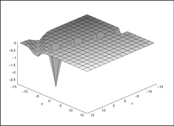
Figure 1: t=-6

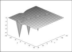
Figure 2: t=-4

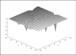
Figure 3: t=-2

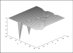
Figure 4: t=2

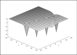
Figure 5: t=4

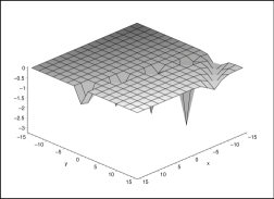
Figure 6: t=6

ii) $N=4$, The Four-Hirota Solution of EKP:

The constants are chosen according to the Case 1 and the dispersion relation. The constants are,

$a=2$, $b=9$, $k_{1}=0$, $k_{2}=0$, $k_{3}=1$, $k_{4}=2$,

$w_{1}=4$, $w_{2}=-2$, $w_{3}=3$, $w_{4}=-5$,

$\displaystyle l_{1}=-6+\frac{2\sqrt{57}}{3}$, $\displaystyle l_{2}=3+\frac{\sqrt{57}}{3}$, $\displaystyle l_{3}=-\frac{9}{2}+\frac{\sqrt{465}}{6}$, $\displaystyle l_{4}=\frac{15}{2}+\frac{\sqrt{1353}}{6}$.

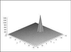
Figure 7: t=-6

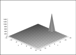
Figure 8: t=-4

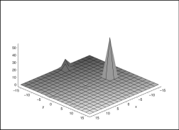
Figure 9: t=-2

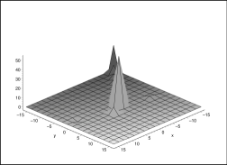
Figure 10: t=2

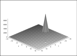
Figure 11: t=4

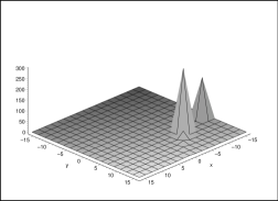
Figure 12: t=6

2.2 The Extended Boussinesq (EBo) Equation

The extended Boussinesq (eBo) equation is given by

$$u_{tt}-u_{xx}+3(u^{2})_{xx}-u_{xxxx}+au_{yy}+bu_{ty}+c\nabla^{2}u=0$$ (49)

which is constructed by adding the terms $au_{yy}$, $bu_{ty}$ and $\nabla^{2}u=u_{x_{1}x_{1}}+u_{x_{2}x_{2}}+...+u_{x_{m}x_{m}}$ multiplied by $c$ to the Boussinesq (Bo) equation where $a$, $b$ and $c$ are constants and $x_{j}$, $j=1,2,...,m$ are independent variables. Now let us apply the Hirota direct method to the eBo equation. Step $1$. Bilinearization: We use the bilinearizing transformation

$$u(x,t,y)=-2\partial_{x}^{2}\log f$$ (50)

so the bilinear form of eBo is

$$ff_{tt}-f_{t}^{2}-f_{xx}f+f_{x}^{2}-f_{xxxx}f+4f_{x}f_{xxx}-3f_{xx}^{2}\\ +af_{yy}f-af_{y}^{2}+bf_{ty}f-bf_{t}f_{y}+c\sum_{j=1}^{m}(f_{x_{j}x_{j}}f-f_{x_{j}}^{2})=0.$$ (51)

Step $2$. Transformation to the Hirota bilinear form: The Hirota bilinear form of eBo is

$$P(D)\{f.f\}=(D_{t}^{2}-D_{x}^{2}-D_{x}^{4}+aD_{y}^{2}+bD_{t}D_{y}+c\sum_{j=1}^{m}D_{x_{j}}^{2})\{f.f\}=0.$$ (52)

Step $3$. Application of the Hirota perturbation: Insert $f=1+\sum_{n=1}^{N}\varepsilon^{n}f_{n}$into the equation (52) so we have

$$P(D)\{f.f\}=P(D)\{1.1\}+\varepsilon P(D)\{f_{1}.1+1.f_{1}\}\\ +...+\varepsilon^{2N}P(D)\{f_{N}.f_{N}\}=0.$$ (53)

Step $4$: Examination of the coefficients of the perturbation parameter $\varepsilon$: We make the coefficients of $\varepsilon^{m}$, $m=1,2,...,N$ appeared in (53) to vanish. Here we shall consider only the case $N=3$ and $N=4$.

2.2.1 $N=3$, Three-Hirota Solution of EBo

Here we apply the Hirota direct method by using the ansatz which is used to construct three-soliton solutions. We take $f=1+\varepsilon f_{1}+\varepsilon^{2}f_{2}+\varepsilon^{3}f_{3}$ where $f_{1}=e^{\theta_{1}}+e^{\theta_{2}}+e^{\theta_{3}}$ with $\theta_{i}=k_{i}x+\omega_{i}t+l_{i}y+\sum_{j=1}^{m}r_{ij}x_{j}+\alpha_{i}$ for $i=1,2,3$ and insert it into (53). The coefficient of $\varepsilon^{0}$ is identically zero. By the coefficient of $\varepsilon^{1}$

$$P(D)\{1.f_{1}+f_{1}.1\}=2P(\partial)\{e^{\theta_{1}}+e^{\theta_{2}}+e^{\theta_{3}}\}=0$$ (54)

we have the dispersion relation

$$P(p_{i})=\omega_{i}^{2}-k_{i}^{2}-k_{i}^{4}+al_{i}^{2}+b\omega_{i}l_{i}+c\sum_{j}^{m}r_{ij}^{2}=0$$ (55)

for $i=1,2,3$. Similar to the eKP equation, we see that when $c$, the coefficient of $\nabla^{2}u$ is not zero, we can apply the Hirota method. But for simplicity we take $c=0$ in the rest of the calculations. In this case $\theta_{i}$ become $\theta_{i}=k_{i}x+\omega_{i}t+l_{i}y+\alpha_{i}$. From the coefficient of $\varepsilon^{2}$ we get

$$-P(\partial)f_{2}=\sum_{i<j}^{(3)}[(\omega_{i}-\omega_{j})^{2}-(k_{i}-k_{j})^{2}-(k_{i}-k_{j})^{4}+a(l_{i}-l_{j})^{2}\\ +b(\omega_{i}-\omega_{j})(l_{i}-l_{j})]e^{\theta_{i}+\theta_{j}}$$ (56)

where $(3)$ indicates the summation of all possible combinations of the three elements with $i<j$. Thus $f_{2}$ should be of the form

$$f_{2}=A(1,2)e^{{\theta_{1}}+{\theta_{2}}}+A(1,3)e^{{\theta_{1}}+{\theta_{3}}}+A(2,3)e^{{\theta_{2}}+{\theta_{3}}}$$ (57)

to satisfy the equation. We insert $f_{2}$ into the equation (56) so we get $A(i,j)$ as

$$\begin{split}A(i,j)&=-\frac{P(p_{i}-p_{j})}{P(p_{i}+P_{j})}\\ &=\displaystyle\frac{2\omega_{i}\omega_{j}-2k_{i}k_{j}-4k_{i}^{3}k_{j}+6k_{i}^{2}k_{j}^{2}-4k_{i}k_{j}^{3}+2al_{i}l_{j}+b\omega_{i}l_{j}+b\omega_{j}l_{i}}{2\omega_{i}\omega_{j}-2k_{i}k_{j}-4k_{i}^{3}k_{j}-6k_{i}^{2}k_{j}^{2}-4k_{i}k_{j}^{3}+2al_{i}l_{j}+b\omega_{i}l_{j}+b\omega_{j}l_{i}}\end{split}$$ (58)

where $i,j=1,2,3$, $i<j$. From the coefficient of $\varepsilon^{3}$, we obtain

$$P(\partial)\{f_{3}\}=-[A(1,2)P(p_{3}-p_{2}-p_{1})+A(1,3)P(p_{2}-p_{1}-p_{3})\\ +A(2,3)P(p_{1}-p_{2}-p_{3})]e^{{\theta_{1}}+{\theta_{2}}+{\theta_{3}}}.$$ (59)

Hence $f_{3}$ is in the form $f_{3}=Be^{{\theta_{1}}+{\theta_{2}}+{\theta_{3}}}$ where $B$ is found as

$$B=\displaystyle-\frac{A(1,2)P(p_{3}-p_{1}-p_{2})+A(1,3)P(p_{2}-p_{1}-p_{3})+A(2,3)P(p_{1}-p_{2}-p_{3})}{P(p_{1}+p_{2}+p_{3})}.$$ (60)

The coefficient of $\varepsilon^{4}$ gives us

$$e^{{2\theta_{1}}+{\theta_{2}}+{\theta_{3}}}[BP(p_{2}+p_{3})+A(1,2)A(1,3)P(p_{2}-p_{3})]\\ +e^{{\theta_{1}}+{2\theta_{2}}+{\theta_{3}}}[BP(p_{1}+p_{3})+A(1,2)A(2,3)P(p_{1}-p_{3})]\\ +e^{{\theta_{1}}+{\theta_{2}}+{2\theta_{3}}}[BP(p_{1}+p_{2})+A(1,3)A(2,3)P(p_{1}-p_{2})]=0$$ (61)

which is satisfied when

$$B=A(1,2)A(1,3)A(2,3).$$ (62)

The two expressions for $B$ should be equivalent. This yields the three-Hirota solution condition $(3HC)$

$$\sum_{\sigma_{r}=\pm 1}P(\sigma_{1}p_{1}+\sigma_{2}p_{2}+\sigma_{3}p_{3})P(\sigma_{1}p_{1}-\sigma_{2}p_{2})P(\sigma_{2}p_{2}-\sigma_{3}p_{3})P(\sigma_{1}p_{1}-\sigma_{3}p_{3})=0,$$ (63)

$r=1,2,3$ which turns out to be the below equation for eBo,

$$\begin{split}&(4a-b^{2})k_{1}^{2}k_{2}^{2}k_{3}^{2}\Big{[}2k_{1}^{2}w_{2}w_{3}l_{2}l_{3}+2k_{2}^{2}w_{1}w_{3}l_{1}l_{3}+2k_{3}^{2}w_{1}w_{2}l_{1}l_{2}\\ &+2k_{2}k_{3}w_{2}w_{3}l_{1}^{2}+2k_{1}k_{3}w_{1}w_{3}l_{2}^{2}+2k_{1}k_{2}w_{1}w_{2}l_{3}^{2}+2k_{2}k_{3}w_{1}^{2}l_{2}l_{3}\\ &+2k_{1}k_{3}w_{2}^{2}l_{1}l_{3}+2k_{1}k_{2}w_{3}^{2}l_{1}l_{2}-2k_{1}k_{3}w_{2}w_{3}l_{1}l_{2}-2k_{1}k_{3}w_{1}w_{2}l_{2}l_{3}\\ &-2k_{1}k_{2}w_{2}w_{3}l_{1}l_{3}-2k_{1}k_{2}w_{1}w_{3}l_{2}l_{3}-2k_{2}k_{3}w_{1}w_{3}l_{1}l_{2}-2k_{2}k_{3}w_{1}w_{2}l_{1}l_{3}\\ &-k_{1}^{2}w_{3}^{2}l_{2}^{2}-k_{1}^{2}w_{2}^{2}l_{3}^{2}-k_{2}^{2}w_{1}^{2}l_{3}^{2}-k_{2}^{2}w_{3}^{2}l_{1}^{2}-k_{3}^{2}w_{2}^{2}l_{1}^{2}-k_{3}^{2}w_{1}^{2}l_{2}^{2}\Big{]}=0.\end{split}$$ (64)

It is satisfied when $a=b^{2}/4$ or for some relations on $k_{i}$, $w_{i}$ and $l_{i}$ which violate the solitonic property of the solution. The coefficients of $\varepsilon^{5}$ and $\varepsilon^{6}$ vanish trivially. Similar to eKP, when $a=b^{2}/4$, eBo is integrable since it is transformable to Bo by the transformation

$u^{\prime}=u$, $x^{\prime}=x$, $y^{\prime}=\alpha t+\beta y$, $t^{\prime}=t+\rho y$,

where $\alpha=b/2=\sqrt{a}$. When $a\neq b^{2}/4$, eBo is not integrable. The other relations which makes $(3HC)$ satisfied are;

Case 1. Any $k_{i}=0$, $i=1,2,3$, the rest are different,

Case 2. $k_{i}=\omega_{i}$, $i=1,2,3$,

Case 3. $k_{i}=l_{i}$, $i=1,2,3$,

Case 4. $\omega_{i}=l_{i}$, $i=1,2,3$.

By using any of these cases, we obtain the exact solutions of eBo.

2.2.2 $N=4$, Four-Hirota Solution of EBo

Here we apply the Hirota direct method by using the ansatz which is used to construct four-soliton solutions. We take $f=1+\varepsilon f_{1}+\varepsilon^{2}f_{2}+\varepsilon^{3}f_{3}+\varepsilon^{4}f_{4}$ where $f_{1}=e^{\theta_{1}}+e^{\theta_{2}}+e^{\theta_{3}}+e^{\theta_{4}}$ with $\theta_{i}=k_{i}x+\omega_{i}t+l_{i}y+\alpha_{i}$ for $i=1,2,3,4$ and insert it into (53). We will only consider the coefficients of $\varepsilon^{m}$, $m=1,2,3,4,5$ since the others vanish identically. By the coefficient of $\varepsilon^{1}$

$$P(D)\{1.f_{1}+f_{1}.1\}=2P(\partial)\{e^{\theta_{1}}+e^{\theta_{2}}+e^{\theta_{3}}+e^{\theta_{4}}\}=0$$ (65)

we have the dispersion relation

$$P(p_{i})=\omega_{i}^{2}-k_{i}^{2}-k_{i}^{4}+al_{i}^{2}+b\omega_{i}l_{i}=0$$ (66)

for $i=1,2,3,4$. From the coefficient of $\varepsilon^{2}$ we obtain

$$-P(\partial)f_{2}=P(p_{1}-p_{2})e^{\theta_{1}+\theta_{2}}+P(p_{1}-p_{3})e^{\theta_{1}+\theta_{3}}+P(p_{1}-p_{4})e^{\theta_{1}+\theta_{4}}\\ +P(p_{2}-p_{3})e^{\theta_{2}+\theta_{3}}+P(p_{2}-p_{4})e^{\theta_{2}+\theta_{4}}+P(p_{3}-p_{4})e^{\theta_{3}+\theta_{4}}.$$ (67)

Thus $f_{2}$ should be of the form

$$f_{2}=A(1,2)e^{{\theta_{1}}+{\theta_{2}}}+A(1,3)e^{{\theta_{1}}+{\theta_{3}}}+A(1,4)e^{\theta_{1}+\theta_{4}}\\ +A(2,3)e^{{\theta_{2}}+{\theta_{3}}}+A(2,4)e^{\theta_{2}+\theta_{4}}+A(3,4)e^{\theta_{3}+\theta_{4}},$$ (68)

where $A(i,j)$ are obtained as

$$\begin{split}A(i,j)&=-\frac{P(p_{i}-p_{j})}{P(p_{i}+P_{j})}\\ &=\displaystyle\frac{2\omega_{i}\omega_{j}-2k_{i}k_{j}-4k_{i}^{3}k_{j}+6k_{i}^{2}k_{j}^{2}-4k_{i}k_{j}^{3}+2al_{i}l_{j}+b\omega_{i}l_{j}+b\omega_{j}l_{i}}{2\omega_{i}\omega_{j}-2k_{i}k_{j}-4k_{i}^{3}k_{j}-6k_{i}^{2}k_{j}^{2}-4k_{i}k_{j}^{3}+2al_{i}l_{j}+b\omega_{i}l_{j}+b\omega_{j}l_{i}}\end{split}$$ (69)

for $i,j=1,2,3,4$ with $i<j$. The coefficient of $\varepsilon^{3}$ gives

$$-P(\partial)f_{3}=\sum_{i<j<m}^{(4)}[A(i,j)P(p_{m}-p_{i}-p_{j})+A(i,m)P(p_{j}-p_{i}-p_{m})\\ +A(j,m)P(p_{i}-p_{j}-p_{m})]e^{\theta_{i}+\theta_{j}+\theta_{m}}$$ (70)

where $(4)$ indicates the summation of all possible combinations of the four elements with $i<j<m$. Hence $f_{3}$ is of the form

$$f_{3}=B(1,2,3)e^{{\theta_{1}}+{\theta_{2}}+{\theta_{3}}}+B(1,2,4)e^{{\theta_{1}}+{\theta_{2}}+{\theta_{4}}}\\ +B(1,3,4)e^{{\theta_{1}}+{\theta_{3}}+{\theta_{4}}}+B(2,3,4)e^{{\theta_{2}}+{\theta_{3}}+{\theta_{4}}}.$$ (71)

$B(i,j,m)$ are obtained as

$$B(i,j,m)=\displaystyle-\frac{A(i,j)P(p_{m}-p_{i}-p_{j})+A(i,m)P(p_{j}-p_{i}-p_{m})+A(j,m)P(p_{i}-p_{j}-p_{m})}{P(p_{i}+p_{j}+p_{m})}$$ (72)

for $i,j,m=1,2,3,4$ with $i<j<m$. From the coefficient of $\varepsilon^{4}$ we have

$$\begin{split}P(D)\{f_{4}.1+f_{3}.f_{1}+f_{2}.f_{2}+f_{1}.f_{3}+1.f_{4}\}&=2P(\partial)f_{4}+2P(D)\{f_{1}.f_{3}\}+P(D)\{f_{2}.f_{2}\}\\ &=0.\end{split}$$ (73)

After simplifications we see that we should have

$$B(i,j,m)=A(i,j)A(i,m)A(j,m)$$ (74)

for $i,j,m=1,2,3,4$ with $i<j<m$. To be consistent the equations (72) and (74) should be equivalent. This gives us the condition

$$\sum_{\sigma_{r}=\pm 1}P(\sigma_{i}p_{i}+\sigma_{j}p_{j}+\sigma_{m}p_{m})P(\sigma_{i}p_{i}-\sigma_{j}p_{j})P(\sigma_{j}p_{j}-\sigma_{m}p_{m})P(\sigma_{i}p_{i}-\sigma_{m}p_{m})=0.$$ (75)

for $i,j,m,r=1,2,3,4$ with $i<j<m$, which becomes

$$\begin{split}&(4a-b^{2})k_{i}^{2}k_{j}^{2}k_{m}^{2}\Big{[}2k_{i}^{2}w_{j}w_{m}l_{j}l_{m}+2k_{j}^{2}w_{i}w_{m}l_{i}l_{m}+2k_{m}^{2}w_{i}w_{j}l_{i}l_{j}\\ &+2k_{j}k_{m}w_{j}w_{m}l_{i}^{2}+2k_{i}k_{m}w_{i}w_{m}l_{j}^{2}+2k_{i}k_{j}w_{i}w_{j}l_{m}^{2}+2k_{j}k_{m}w_{i}^{2}l_{j}l_{m}\\ &+2k_{i}k_{m}w_{j}^{2}l_{i}l_{m}+2k_{i}k_{j}w_{m}^{2}l_{i}l_{j}-2k_{i}k_{m}w_{j}w_{m}l_{i}l_{j}-2k_{i}k_{m}w_{i}w_{j}l_{j}l_{m}\\ &-2k_{i}k_{j}w_{j}w_{m}l_{i}l_{m}-2k_{i}k_{j}w_{i}w_{m}l_{j}l_{m}-2k_{j}k_{m}w_{i}w_{m}l_{i}l_{j}-2k_{j}k_{m}w_{i}w_{j}l_{i}l_{m}\\ &-k_{i}^{2}w_{m}^{2}l_{j}^{2}-k_{i}^{2}w_{j}^{2}l_{m}^{2}-k_{j}^{2}w_{i}^{2}l_{m}^{2}-k_{j}^{2}w_{m}^{2}l_{i}^{2}-k_{m}^{2}w_{j}^{2}l_{i}^{2}-k_{m}^{2}w_{i}^{2}l_{j}^{2}\Big{]}=0\end{split}$$ (76)

where $i,j,m=1,2,3,4$, $i<j<m$. Some of the cases except $a=b^{2}/4$ which make this condition holds are;

Case 1. Any two of $k_{i}=0$, $i=1,2,3,4$, the rest are different,

Case 2. $k_{i}=\omega_{i}$, $i=1,2,3,4$,

Case 3. $k_{i}=l_{i}$, $i=1,2,3,4$,

Case 4. $\omega_{i}=l_{i}$, $i=1,2,3,4$.

The equation remaining from the coefficient of $\varepsilon^{4}$ is

$$-P(\partial)f_{4}=e^{\theta_{1}+\theta_{2}+\theta_{3}+\theta_{4}}[B_{123}P(p_{4}-p_{1}-p_{2}-p_{3})+B_{124}P(p_{3}-p_{1}-p_{2}-p_{4})]\\ +B_{134}P(p_{2}-p_{1}-p_{3}-p_{4})+B_{234}P(p_{1}-p_{2}-p_{3}-p_{4})+A(1,2)A(3,4)P(p_{1}+p_{2}-p_{3}-p_{4})\\ +A(1,3)A(2,4)P(p_{1}+p_{3}-p_{2}-p_{4})+A(1,4)A(2,3)P(p_{1}+p_{4}-p_{2}-p_{3})]=0.$$ (77)

Hence $f_{4}=Ce^{\theta_{1}+\theta_{2}+\theta_{3}+\theta_{4}}$ where $C$ is obtained as

$$\begin{split}C=-[&A(1,2)A(3,4)P(p_{1}+p_{2}-p_{3}-p_{4})+A(1,3)A(2,4)P(p_{1}+p_{3}-p_{2}-p_{4})\\ +&A(1,4)A(2,3)P(p_{1}+p_{4}-p_{2}-p_{3})+B(1,2,3)P(p_{4}-p_{1}-p_{2}-p_{3})\\ +&B(1,2,4)P(p_{3}-p_{1}-p_{2}-p_{4})+B(1,3,4)P(p_{2}-p_{1}-p_{3}-p_{4})\\ +&B(2,3,4)P(p_{1}-p_{2}-p_{3}-p_{4})]\Bigg{/}P(p_{1}+p_{2}+p_{3}+p_{4}).\end{split}$$ (78)

From the coefficient of $\varepsilon^{5}$ we have

$$2P(\partial)f_{4}+2P(D)\{f_{1}.f_{3}\}+P(D)\{f_{2}.f_{2}\}=0.$$ (79)

The simplifications give us that

$$C=A(1,2)A(1,3)A(1,4)A(2,3)A(2,4)A(3,4).$$ (80)

To be consistent the equations (78) and (80) should be equal to each other. This yields the four-Hirota solution condition $(4HC)$

$$\sum_{\sigma_{i}=\pm 1}P(\sum_{i=1}^{4}\sigma_{i}p_{i})\prod_{0<i<j<4}[P(\sigma_{i}p_{i}-\sigma_{j}p_{j})]=0.$$ (81)

In the hand, we know a case which satisfies both $(3HC)$ and $(4HC)$ automatically which is

Case 1. Any two of $k_{i}=0$, $i=1,2,3,4$, the rest are different.

Here we give the graphs of the two- and four-Hirota solutions of eBo. We give arbitrary values to $a$, $b$, $k_{i}$ and $w_{i}$. From the dispersion relation, we obtain $l_{i}$. We use these constants in the solutions and draw their graphs.

i) $N=2$, The Two-Hirota Solution of EKP:

The constants are

$a=5$, $b=8$, $k_{1}=1$, $k_{2}=2$,

$w_{1}=-3$, $w_{2}=-5$, $\displaystyle l_{1}=\frac{12+\sqrt{109}}{5}$, $\displaystyle l_{2}=4-\sqrt{15}$.

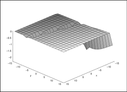
Figure 13: t=-6

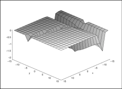
Figure 14: t=-4

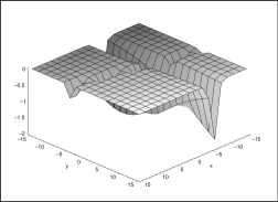
Figure 15: t=-2

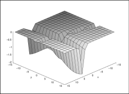
Figure 16: t=2

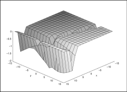
Figure 17: t=4

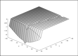
Figure 18: t=6

ii) $N=4$, The Four-Hirota Solution of EBo:

The constants are chosen according to the Case 1 and the dispersion relation. The constants are,

$a=5$, $b=8$, $k_{1}=0$, $k_{2}=0$, $k_{3}=2$, $k_{4}=3$,

$w_{1}=5$, $w_{2}=4$, $w_{3}=-6$, $w_{4}=1$,

$\displaystyle l_{1}=-4+\sqrt{11}$, $\displaystyle l_{2}=\frac{-16-4\sqrt{11}}{5}$, $\displaystyle l_{3}=\frac{24+4\sqrt{31}}{5}$, $\displaystyle l_{4}=\frac{-4-\sqrt{461}}{5}$.

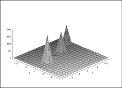
Figure 19: t=-6

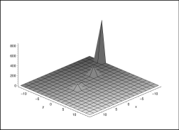
Figure 20: t=-4

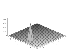
Figure 21: t=-2

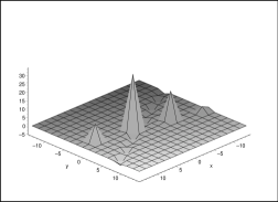
Figure 22: t=2

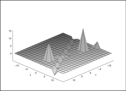
Figure 23: t=4

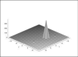
Figure 24: t=6

3 Conclusion

In this work, we applied the Hirota direct method to non-integrable equations. We have given two examples, the extended Kadomtsev-Petviashvili (eKP) and the extended Boussinesq equations. They are in general non-integrable equations.

We have written bilinear and Hirota bilinear forms of these equations. Since the equations having Hirota bilinear forms automatically possess one- and two-Hirota solutions ( which have soliton-like behavior), we have focused on three- and four-Hirota solutions. We have seen that both equations should satisfy a condition which we call three-Hirota solution condition $(3HC)$ to have three-Hirota solution. While trying to obtain four-Hirota solutions of the equations we have come across another condition, four-Hirota solution condition $(4HC)$. We have classes of solutions of these two conditions.

References

- [1] Hirota R., Exact solution of the Korteweg-de Vries equation for multiple collisions of solitons, Phys. Rev. Lett., 27, 1192 (1971).
- [2] Hirota R., Exact solution of the modified Korteweg-de Vries equation for multiple collisions of solitons, J. Phys. Soc. Japan, 33, 1456 (1972).
- [3] Hirota R., Exact solution of the sine-Gordon equation for multiple collisions of solitons, J. Phys. Soc. Japan, 33, 1459 (1972).
- [4] Hirota R., Exact envelope-soliton solutions of a nonlinear wave equation, J. Math. Phys, 14, 805-809 (1973).
- [5] Hirota R., Exact N-soliton solution of a nonlinear lumped network equation, J. Phys. Soc. Japan, 35, 286-288 (1973).
- [6] Grammaticos B., Ramani A. and Hietarinta J., Multilinear operators: the natural extension of Hirota’s bilinear formalism, Phys. Lett. A, 190, 65-70 (1994).
- [7] Hietarinta J., Searching for integrable PDE’s by testing Hirota’s three-soliton condition, Proceedings of the 1991 International Symposium on Symbolic and Algebraic Computation, ISSAC’91”, Stephen M. Watt, (Association for Computing Machinery, 1991), 295-300.
- [8] Hietarinta J., A search of bilinear equations passing Hirota’s three-soliton condition: I. KdV-type bilinear equations, J. Math. Phys. 28, 1732-1742 (1987).
- [9] Hietarinta J., A search of bilinear equations passing Hirota’s three-soliton condition: II. mKdV-type bilinear equations, J. Math. Phys. 28, 2094-2101 (1987).
- [10] Hietarinta J., A search of bilinear equations passing Hirota’s three-soliton condition: III. sine-Gordon-type bilinear equations, J. Math. Phys. 28, 2586-2592 (1987).
- [11] Hietarinta J., A search of bilinear equations passing Hirota’s three-soliton condition: IV. Complex bilinear equations, J. Math. Phys. 29, 628-635 (1988).
- [12] Hietarinta J., Introduction to the bilinear method, in “Integrability of Nonlinear Systems”, eds. Y. Kosman-Schwarzbach, B. Grammaticos and K.M. Tamizhmani, Springer Lecture Notes in Physics 495, 95-103 (1997) arxiv.org/abs/solv-int/9708006.