Beyond scaling and locality in turbulence

Abstract

An analytic perturbation theory is suggested in order to find finite-size corrections to the scaling power laws. In the frame of this theory it is shown that the first order finite-size correction to the scaling power laws has following form $S(r)\cong cr^{\alpha_{0}}[\ln(r/\eta)]^{\alpha_{1}}$, where $\eta$ is a finite-size scale (in particular for turbulence, it can be the Kolmogorov dissipation scale). Using data of laboratory experiments and numerical simulations it is shown shown that a degenerate case with $\alpha_{0}=0$ can describe turbulence statistics in the near-dissipation range $r>\eta$, where the ordinary (power-law) scaling does not apply. For moderate Reynolds numbers the degenerate scaling range covers almost the entire range of scales of velocity structure functions (the log-corrections apply to finite Reynolds number). Interplay between local and non-local regimes has been considered as a possible hydrodynamic mechanism providing the basis for the degenerate scaling of structure functions and extended self-similarity. These results have been also expanded on passive scalar mixing in turbulence. Overlapping phenomenon between local and non-local regimes and a relation between position of maximum of the generalized energy input rate and the actual crossover scale between these regimes are briefly discussed.

I Introduction

Scaling and related power laws are widely used in physics. In real situations, however, scaling holds only approximately. As a consequence, the corresponding scaling power laws hold approximately as well. On the other hand, discovery of the extended self-similarity in turbulence ben1 ,ben2 and in the critical phenomena (see for a review sorn ,mps ) shows that universal laws similar to the scaling ones can go far beyond the scaling itself, both for velocity ben1 ,ben2 and for different fields convected by turbulence astkb ,bs . The question is: does the extended self-similarity (ESS) can be theoretically explored in the frames of general scaling ideas or one needs in a completely new frames to explain the ESS? In turbulence this problem is related to the problem of the so-called near-dissipation range. Theoretical approach to description of the scaling (the so-called inertial) range of scales in turbulence requires that the space scales $r\gg\eta$, where $\eta$ is (Kolmogorov) dissipation or molecular viscous scale sa ; my . On the other hand, the near-dissipation range of scales, for which $r>\eta$ has a more complex, presumably non-scaling dynamics (see, for instance, Refs.nelkin -sb2 and the references cited there). Indeed, for moderate Reynolds numbers, the near-dissipation range can span most of the available range of scales sb . Different perturbation theories, which start from scaling as a leading mode, can be developed. Effectiveness of such theories is usually checked by comparison with experiments. In the present paper we will explore a generic analytic expansion of scaling in direction of the dissipation scale $\eta$. Effectiveness of the suggested perturbation theory has been shown for the turbulent flows with moderate Reynolds numbers. Interplay between local and non-local regimes has been considered as a possible hydrodynamic mechanism providing the basis for the degenerate scaling of structure functions and extended self-similarity in turbulent flows.

II Analytic perturbations to scaling

Let us consider a dimensional function $S(r)$ of a dimensional argument $r$. And let us construct a dimensionless function of the same argument

$$\alpha(r)=\frac{S^{-1}dS}{r^{-1}dr}.$$

If for $L\gg r\gg\eta$ we have no relevant fixed scale (scaling situation), then for these values of $r$ the function $\alpha(r)$ must be independent on $r$, i.e. $\alpha(r)\simeq const$ for $L\gg r\gg\eta$. Solution of equation (1) with constant $\alpha$ can be readily found as

$$S(r)\cong cr^{\alpha}$$

where $c$ is a dimension constant. This is the well-known power law corresponding to the scaling situations.

Let us now consider an analytic theory, which allows us to find generic corrections of all orders to the approximate power law, related to the fixed small scale $\eta$. In the non-scaling situation let us denote

$$f\equiv\ln(S/A),~{}~{}~{}~{}~{}~{}~{}~{}x\equiv\ln(r/\eta)$$

where $A$ and $\eta$ are dimensional constants used for normalization.

In these variables, equation (1) can be rewritten as

$$\frac{df}{dx}=\alpha(x)$$

In the non-scaling situation $x$ is a dimensionless variable, hence the dimensionless function $\alpha(x)$ can be non-constant. Since the ’pure’ scaling corresponds to $x\gg 1$ we will use an analytic expansion in power series

$$\alpha(x)=\alpha_{0}+\frac{\alpha_{1}}{x}+...+\frac{\alpha_{n}}{n!x^{n}}+...$$

where $\alpha_{n}$ are dimensionless constants. After substitution of the analytic expansion (5) into Eq. (4) the zeroth order approximation gives the power law (2) with $\alpha\cong\alpha_{0}$. First order analytic approximation, when one takes only the two first terms in the analytic expansion (5), gives

$$S(r)\cong cr^{\alpha_{0}}[\ln(r/\eta)]^{\alpha_{1}}.$$

This is a generic analytic first order approximation to the scaling power laws provided by the perturbation theory suggested above.

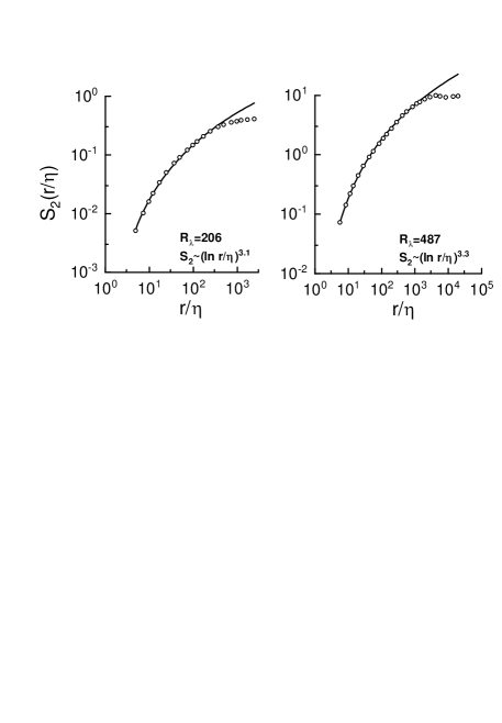
Figure 1: The second order structure function $S_{2}(r/\eta)$ against $r/\eta$. The experimental data ($R_{\lambda}=206,~{}487$) pkw are shown as circles. The solid curves are the best fit of (7) to the data, corresponding to the degenerated scaling.

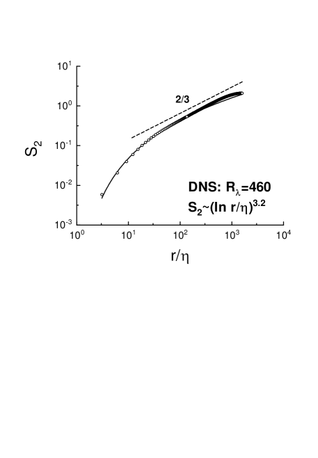
Figure 2: The second order structure function $S_{2}(r/\eta)$ against $r/\eta$. The DNS data gfn ($R_{\lambda}=460$) are shown as circles. The solid curve is the best fit of (7) corresponding to the degenerated scaling.

Corrections of the higher orders can be readily found in this perturbation theory.

For degenerate case with $\alpha_{0}=0$ the second term in the expansion (5) becomes the leading term

$$S(r)\sim[\ln(r/\eta)]^{\alpha_{1}}$$

It was already mentioned that there are many different ways to develop perturbation theory to scaling. The idea that just $\ln(r/\eta)$ is an appropriate parameter for the finite-size corrections to scaling in turbulence was suggested in sb2 . On a physical level this was related in sb2 to the instabilities of the thin vortex tubes (or filaments), which are the most prominent hydrodynamical elements of turbulent flows. These instabilities usually appear as kinks readily transforming into wave packets propagating along the filaments. One can consider such wave packet with scale $r$ and make use of the “localized induction” approximation to the Biot-Savart formula batc . In this approximation, contributions of portions at distances greater than $\sim r\gg\eta$ to the velocity fluctuation in the immediate vicinity of any given point on the filament are neglected. The vortex core radius, which usually associated with $\eta$, provides a cutoff from below. The vortex filament dynamics in this approximation is described by the equation

$$\frac{d{\bf X}}{dt}=\frac{\Gamma}{4\pi}\left\{\ln\left(\frac{r}{\eta}\right)\right\}\gamma{\bf b}$$

where ${\bf X}$ is the position vector of a point on the filament, $\Gamma$ is the vortex strength, $\gamma$ is the local curvature, and ${\bf b}$ is the unit binormal vector of the filament. One can see that in this approximation the dependence on $r$ is completely determined by the logarithmic term $\ln(r/\eta)$ in the dynamic equation. This pure hydrodynamic consideration was suggested in sb2 as a basis for using just $\ln(r/\eta)$ in finite-size corrections to scaling in turbulence (see also Section IV below).

III Turbulence

The longitudinal structure function of order $p$ for the velocity field my

$$S_{p}(r)=\langle|\Delta u|^{p}\rangle$$

($\Delta u=({\bf u}({\bf r}+{\bf x})-{\bf u}({\bf r}))\cdot{\bf r}/r$) calculated for $p=2$, using the data obtained in a wind tunnel at $R_{\lambda}=206$ and 487 pkw , is shown in Fig. 1. Here $R_{\lambda}$ is the so-called Taylor microscale Reynolds number. The experiment with a flow, which was a combination of the wake and homogeneous turbulence behind a grid, is described in Ref. pkw . We invoke Taylor’s hypothesis my to equate temporal statistics to spatial statistics.

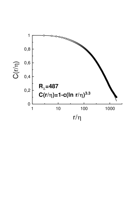
Figure 3: Correlation function for velocity fluctuations against $\log r/\eta$ for $R_{\lambda}=487$ (circles) pkw . The solid curve is drawn in the figure to indicate agreement with the degenerate scaling shown in Fig. 1.

The solid curves in these figures are the best fit by equation (7) corresponding to the degenerate scaling. Figure 2 shows $S_{2}(r)$ calculated using data from a high-resolution direct numerical simulation of homogeneous steady three-dimensional turbulence gfn , corresponding to $1024^{3}$ grid points and $R_{\lambda}=460$. The solid curve in this figure also corresponds to the best fit by equation (7). As far as we know Eq. (7) was suggested as an empirical approximation of the structure functions for the first time in our earlier paper sb . Application of these results to correlation functions my is in good agreement with the structure functions analysis (cf. for instance, Figs. 1 and 3).

Figure 4 shows the structure functions of different orders $p$ for the wind-tunnel data ($R_{\lambda}=487)$ and the degenerate scaling (7) is shown in the figure as the solid curves. One can see that the degenerate scaling requires two fitting constants just as the ordinary scaling does, and, in the examples discussed above, the range of scales covered by the degenerate scaling is about two decades.

IV A possible hydrodynamic scenario

In order to understand a possible hydrodynamic mechanism of the phenomenon described above let us recall that in isotropic turbulence a complete separation of local and non-local interactions is possible in principle. It was shown by Kadomtsev kad that this separation plays a crucial role for the local Kolmogorov’s cascade regime with scaling energy spectrum

$$E(k)\sim\bar{\varepsilon}^{2/3}k^{-5/3}$$

where $\bar{\varepsilon}$ is the average of the energy dissipation rate, $\varepsilon$, $k\sim 1/r$ is the wave-number. This separation should be effective for the both ends. That is, if there exists a solution with the local scaling (9) as an asymptote, then there should also exist a solution with the non-local scaling asymptote. Of course, the two solutions with these asymptotes should be alternatively stable (unstable) in different regions of scales. It is expected, that the local (Kolmogorov’s) solution is stable (i.e. statistically dominating) in inertial range (that means instability of the non-local solution in this range of scales).

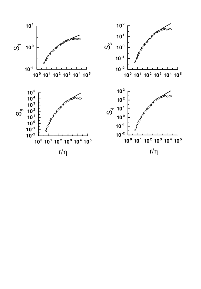
Figure 4: As in Fig. 1 ($R_{\lambda}=487$) but for different orders of the structure function.

Roughly speaking, in non-local solution for small scales $r$ only non-local interactions with large scales $L$ ($1\gg r/L$) are dynamically significant and the non-local interactions is determined by large scale strain/shear. This means that one should add to the energy flux $\bar{\varepsilon}$-parameter (which is a governing parameter for the both solutions) an additional parameter such as the strain $s$ for the non-local solution. As far as we know it was noted for the first time by Nazarenko and Laval nl that dimensional considerations applied to the non-local asymptotic result in the power-law energy spectrum

$$E(k)\sim\frac{\bar{\varepsilon}}{s}~{}k^{-1}$$

both for two- and three-dimensional cases. Linear dependence of the spectrum (10) on $\bar{\varepsilon}$ is determined by the linear nature of equations corresponding to the non-local asymptotic that together with the dimensional considerations results in (10) nl . Interesting numerical simulations were performed in ldn . In these simulations local and non-local interactions have been alternatively removed. For the first case a tendency toward a spectrum flatter than ’-5/3’ is observed near and beyond the separating scale (beyond which local interactions are ignored), that supports Eq. (10) (see also below).

Following to the perturbation theory suggested in Section II both local and non-local regimes can be corrected. The first order correction is

$$E(k)\sim k^{-5/3}[\ln(k_{d}/k)]^{\gamma}$$

and

$$E(k)\sim k^{-1}[\ln(k_{d}/k)]^{\beta}$$

(where $k_{d}\equiv 1/\eta$) for the local and non-local regimes respectively ($\gamma$ and $\beta$ are dimensionless constants). In the case when $\beta\gg\gamma$ the fist order finite-size correction in the non-local regime becomes substantial much ’earlier’ (i.e. for smaller $k$) than for the local (Kolmorov’s) regime (see Eq. (5)). This can result in viscous stabilization of the non-local regime (cf ldn ) and, as a consequence, in the so-called ’exchange of stability’ phenomenon at certain $k_{c}=1/r_{c}$. That is, for $k<k_{c}$ the Kolmogorov’s regime is stable and the non-local regime is unstable, whereas for $k>k_{c}$ the Kolmogorov’s regime is unstable and the non-local regime is stable. For this scenario, at $k=k_{c}$ the Kolmogorov’s regime is still asymptotically scale-invariant (i.e. Eq. (9) gives an adequate approximation for this regime), while for the non-local regime the first order correction is substantial (i.e. Eq. (12) should be used at $k=k_{c}$ for the non-local regime). In this scenario the Kolmogorov’s regime plays significant role in the viscous stabilization of the non-local regime for $k>k_{c}$ (cf ldn ), but for these $k$ the non-local regime becomes statistically dominating instead of the Kolmogorov’s one.

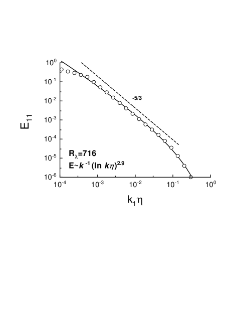
Figure 5: Longitudinal energy spectrum against $k\eta$ in log-log scales. The data (circles) correspond to a nearly isotropic (active-) grid turbulence $R_{\lambda}=716$ kcm . The solid curve is drawn in the figure to indicate agreement with the Eq. (12), while the dashed straight line indicates the ”-5/3” Kolmogorov’s law.

Figure 5 shows a spectrum measured in nearly isotropic turbulence downstream of an active grid at $R_{\lambda}=716$ (the data are reported in kcm ). The solid curve is drawn in the figure to indicate correspondence of the data to the equation (12) (non-local regime), while the dashed straight line indicates the Kolmogorov’s ”-5/3” law to show possible interplay between the Kolmogorov’s and non-local regimes at this Reynolds number.

If one tries to estimate the second order structure function $S_{2}(r)$ as my

$$S_{2}(r)\sim\int_{1/r}^{1/\eta}E(k)dk$$

for $r<r_{c}$ using Eq. (12), one obtains

$$S_{2}(r)\sim[\ln(r/\eta)]^{\zeta_{2}}$$

with $\zeta_{2}=\beta+1$ (cf Section 3). For instance, for the data shown in Fig. 5 we obtain $\zeta_{2}\simeq 3.9$. Comparing figures 1,2 and 5 one can see that $\alpha$ is monotonically increased with $Re_{\lambda}$.

Let us generalize (13) introducing an effective spectrum $E_{n}(k)$

$$S_{n}(r)\sim\int_{1/r}^{1/\eta}E_{n}(k)dk$$

($E_{2}(k)\equiv E(k)$). Then using the dimensional considerations we obtain for the non-local regime

$$E_{n}(k)\sim\left(\frac{\bar{\varepsilon}}{s}\right)^{n/2}~{}k^{-1}$$

The first order correction is

$$E_{n}(k)\sim\left(\frac{\bar{\varepsilon}}{s}\right)^{n/2}~{}k^{-1}[\ln(k_{d}/k)]^{\beta_{n}}$$

Substituting (17) into (15) one obtains

$$S_{n}(r)\sim\left(\frac{\bar{\varepsilon}}{s}\right)^{n/2}~{}[\ln(r/\eta)]^{\zeta_{n}}$$

with $\zeta_{n}=\beta_{n}+1$.

Thus the non-local regime can provide hydrodynamic basis for the degenerate scaling of the structure functions.

V Extended Self-Similarity

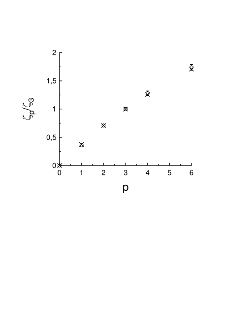
Figure 6: Normalized exponents $\zeta_{p}/\zeta_{3}$ against $p$ for $R_{\lambda}=487$ (circles). The exponents were obtained using the data shown in Figs. 1,4. Crosses are the ESS exponents obtained for the atmospheric turbulence data at $R_{\lambda}=10340$ sd .

In our previous paper sb we discussed possible relation between ESS and structure functions given by Eq. (7). Now we can elaborate this relation with more details. While in the near-dissipation range we observe the degenerate scaling an ordinary scaling (presumably Kolmogorov’s one) has been certainly observed in the inertial range of scales for very large Reynolds numbers (see, for instance, my ,sd ). Therefore, one can expect the existence of a crossover scale $r_{c}$ from the ordinary scaling to the degenerate one (see previous section). At the scale $r=r_{c}$ we can use a continuity condition between ordinary scaling (2) and degenerate scaling (7)

$$cr_{c}^{\zeta^{\prime}_{2}}=A[\ln(r_{c}/\eta]^{\zeta_{2}}$$

for the structure functions of all orders ($c$ and $A$ are some constants). Let us denote in general case

$$S_{p}(r)=A_{p}^{\prime}r^{\zeta_{p}^{\prime}};~{}~{}~{}~{}~{}S_{p}(r)=A_{p}[\ln(r/\eta)]^{\zeta_{p}}$$

in inertial and near-dissipation ranges respectively.

Then condition of compatibility of the continuity equations (19) for different order ($m$ and $n$) structure functions

$$A_{m}^{\prime}r_{c}^{\zeta_{m}^{\prime}}=A_{m}[\ln(r_{c}/\eta)]^{\zeta_{m}};~{}~{}~{}A_{n}^{\prime}r_{c}^{\zeta_{n}^{\prime}}=A_{n}[\ln(r_{c}/\eta)]^{\zeta_{n}}$$

can be of two kinds.

The first kind is applicable for arbitrary value of $r_{c}$ and has the form

$$\frac{\zeta_{m}}{\zeta_{n}}=\frac{\zeta_{m}^{\prime}}{\zeta_{n}^{\prime}};~{}~{}~{}~{}~{}\left(\frac{A_{m}^{\prime}}{A_{m}}\right)^{\zeta_{n}}=\left(\frac{A_{n}^{\prime}}{A_{n}}\right)^{\zeta_{m}}$$

while another kind is applicable for a fixed value of $r_{c}$ only. Below we will be interested in the first kind of the compatibility condition. This condition, in particular, gives a power-law relation between moments of different orders

$$S_{m}(r)\sim S_{n}^{\beta_{m,n}}(r),$$

with the same exponent

$$\beta_{m,n}=\frac{\zeta_{m}^{\prime}}{\zeta_{n}^{\prime}}=\frac{\zeta_{m}}{\zeta_{n}}$$

for both inertial and near-dissipation ranges (see Eq. (22)). The last phenomenon was previously observed in different turbulent flows and was called Extended Self-Similarity (ESS) ben1 ,ben2 ,sb . It is important to note that at ESS not only the scalings (23) are the same in both regimes inertial and dissipative, but also the prefactors are the same. Figure 6 shows as circles the exponents $\zeta_{p}$ obtained from Figs. 1,4 and normalized by the exponent $\zeta_{3}$. For comparison we show by crosses in this figure the normalized exponents obtained using ESS in the atmospheric turbulence for large $R_{\lambda}=10340$ sd .

It should be noted that a high-resolution numerical simulation reported in a recent paper sys for low-Reynolds-number ($R_{\lambda}\approx 10-60$) flows shows no hint of scaling-like behavior of the velocity increments even when ESS is applied. That should return us to the Section II and recall us that the degenerate scaling in the form of Eq. (7) is only a first non-trivial term in the perturbation theory. Moreover, the question of convergence of the perturbation theory used in Section II become significant at the low-Reynolds-number, when the dissipation scale is effectively too close to the scales under consideration. Though, the authors of Ref. sys claim that: ’the DNS scaling exponents of velocity gradients agree well with those deduced, using a recent theory of anomalous scaling, from the scaling exponents of the longitudinal structure functions at infinitely high Reynolds numbers. This suggests that the asymptotic state of turbulence is attained for the velocity gradients at far lower Reynolds numbers than those required for the inertial range to appear’. This circle of problems can be also related to the possibility of fluctuations of the dissipation scale sys ,y . For the cases when these fluctuations are significant a set of the expansions might be needed or (alternatively, for moderate Reynolds numbers) calculation should involve averaging over the fluctuating cut-off $\eta$. In the last case the experimental and numerical data suggest that the average value of $\eta$ should not deviate strongly from the Kolmogorov dissipation scale (at least for the moderate values of Reynolds number).

Though, the problem with the small Reynolds numbers can be deeper. We do not know whether the non-local regime appears at the same Reynolds number as the local one. The energy balance of the non-local regime is more complex than that of the local one. Actually the non-local regime needs in the local one (even statistically unstable) for this balance (cf ldn ). Therefore, critical Reynolds number for appearance of the (stable) non-local regime can be larger than that for the local regime.

VI Generalized energy input rate

Figures 2 and 5 show that for sufficiently large Reynolds numbers, providing a visible inertial interval, there is an overlapping between the two scalings: non-local and local (Kolmogorov). This overlapping is based on the very nature of the stability exchange between the two statistical regimes. Therefore, it is not a simple task to determine the scale $r_{c}$ from the $S_{n}(r)$-data. A more fine information one can infer studying

$$D_{LLL}(r)=\langle\Delta u^{3}\rangle$$

(cf Eq.(8) and see my ,sb2 ,gfn ). Unlike $S_{3}$ most positive contributions are canceled by negative ones in $D_{LLL}$, and only the slight asymmetry of the $\Delta u$ probability density contributes to $D_{LLL}$. However, this asymmetry has a fundamental nature. Therefore, one can expect that the above used dimensional considerations can be also used for $D_{LLL}$ for the both non-local and local regimes. For the local (Kolmogorov) regime one has my ,sb2 ,gfn

$$-D_{LLL}\sim\bar{\varepsilon}~{}r$$

while for the degenerate scaling

$$-D_{LLL}\sim\ \left(\frac{\bar{\varepsilon}}{s}\right)^{3/2}~{}[\ln(r/\eta)]^{\delta}$$

Figure 7 shows $-D_{LLL}$ (as circles) and $-D_{LLL}/\bar{\varepsilon}r$ (as crosses) calculated using data from the direct numerical simulation of homogeneous steady three-dimensional turbulence gfn . The solid curve in this figure corresponds to the best fit by equation (26). In this figure one can see that the overlapping between the two regimes exists even for the $D_{LLL}$ (cf Fig. 2). However, a generalized energy input rate related to $D_{LLL}$ sb2 could give a key to our problem.

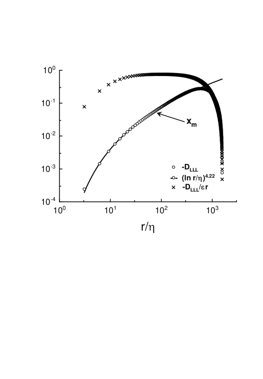
Figure 7: The DNS data gfn ($R_{\lambda}=460$) are shown against $r/\eta$ as the symbols: $-D_{LLL}$-circles and $-D_{LLL}/\bar{\varepsilon}r$-crosses. The solid curve is the best fit of (26) corresponding to the degenerated scaling.

Let us consider the Navier-Stokes equations for a viscous incompressible fluid, given by

$$\frac{\partial u_{i}}{\partial t}+u_{j}\frac{\partial u_{i}}{\partial x_{j}}=-\frac{1}{\rho}\frac{\partial p}{\partial x_{i}}+\nu\frac{\partial^{2}u_{i}}{\partial x_{j}^{2}}+f_{i}({\bf x},t),$$

$$\frac{\partial u_{i}}{\partial x_{i}}=0,$$

where ${\bf f}({\bf x},t)$ is random force, $\nu$ is kinematic viscosity and $\rho$ is the fluid density. $\bf f$ will be assumed to be Gaussian with zero mean and a rapidly oscillating character, or a $\delta$-correlation in time. The second-rank correlation tensor

$$\langle f_{i}({\bf x}+{\bf r},t+\tau)f_{j}({\bf x},t)\rangle\sim F_{ij}({\bf r})\delta(\tau).$$

defines such fields.

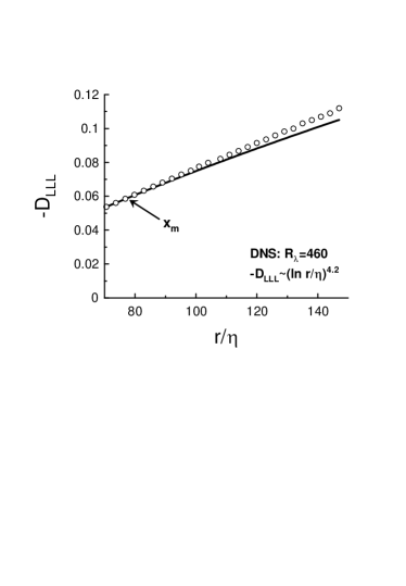
Figure 8: $-D_{LLL}$ against $r/\eta$. The same data as in Fig. 7 but with higher resolution in a small vicinity of the $x_{m}$ scale. The solid curve is the best fit of (26) corresponding to the degenerate scaling.

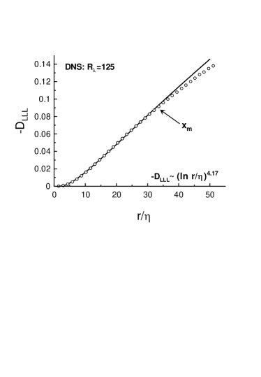
Figure 9: The same as in Fig. 8 but for $R_{\lambda}=125$.

It was shown in nov using Eqs. (27) and (28) that $S_{2}$ and $D_{LLL}$ are related by the equation

$$D_{LLL}=6\nu\frac{dS_{2}}{dr}-\frac{2}{r^{4}}\int_{0}^{r}x^{4}F_{ii}(x)dx,$$

It was also shown in nov that

$$F_{ii}(0)=2\langle\bar{\varepsilon}\rangle.$$

$F_{ii}$ corresponds to an external energy input rate nov (cf Novikov’s relation nov : $\langle f_{i}({\bf x},t)v_{j}({\bf x}^{\prime},t)\rangle=\frac{1}{2}~{}F_{ij}({\bf x}-{\bf x}^{\prime})$).

For $r\ll L$ nov

$$D_{LLL}\simeq 6\nu\frac{dS_{2}}{dr}-\frac{4}{5}\langle\bar{\varepsilon}\rangle r.$$

When the viscous term can be neglected this gives the Kolmogorov’s law (25).

One can formally rewrite (29) as

$$D_{LLL}=-\frac{2}{r^{4}}\int_{0}^{r}x^{4}\tilde{F}(x)dx,$$

where the generalized energy input rate is defined as sb2

$$\tilde{F}(x)\equiv F_{ii}(x)-\frac{3\nu}{x^{4}}\frac{d(x^{4}dS_{2}/dx)}{dx}.$$

Without the second (viscous) term in the right-hand side of Eq. (33) one obtains the Kolmogorov law (25). Therefore, one can associate the first term in the right-hand side of the Eq. (33) with the local (Kolmogorov) regime while the second term can be associated with the non-local one. Gradients of these terms can be associated with local and non-local interaction strengths respectively. Then balance of the local and non-local interaction strengths should be reached at the point given by the equation $d\tilde{F}(x)/dx=0$. Let us denote position of the balance point as $x=x_{m}$. One can expect that the crossover scale $r_{c}$ between the local and non-local regimes (see Section IV) coincides with the balance point of the local and non-local interaction strengths $x_{m}$, i.e. $r_{c}=x_{m}$. It was shown in sb2 that position of the generalized energy input rate maximum $x_{m}\cong r_{m}/1.22$, where $r_{m}$ is position of $-D_{LLL}(r)$ maximum. Since $r_{m}$ can be obtained from the data this gives us a possibility to estimate $r_{c}$ from the data as well. For instance, we know sb2 that $r_{m}/\eta\sim R_{\lambda}^{0.7}$, hence $r_{c}/\eta\sim R_{\lambda}^{0.7}$.

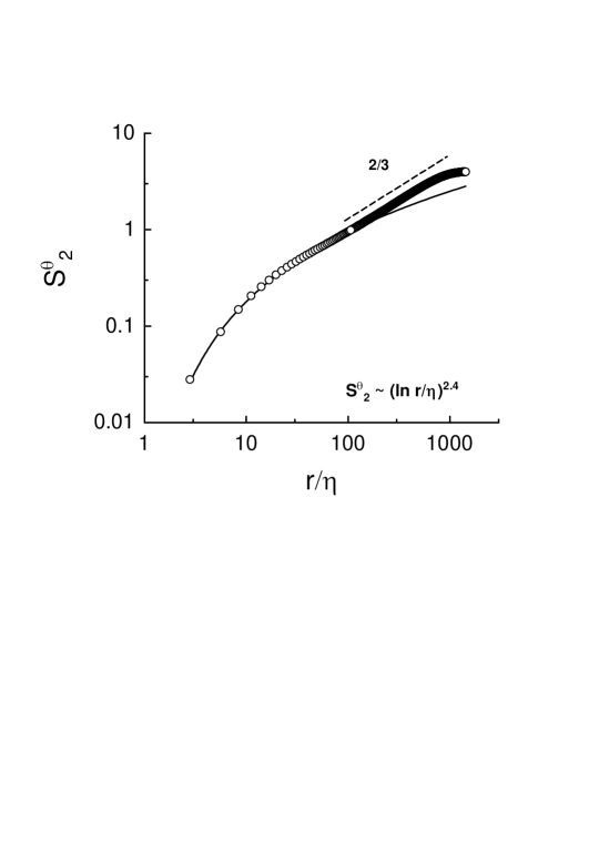
Figure 10: $S^{\theta}_{2}$ against $r/\eta$. The DNS data (circles) of homogeneous isotropic turbulence described in wg , Péclet number $P_{\lambda}=427$ and the Schmidt number is unity (i.e $P_{\lambda}=R_{\lambda}$). The solid curve is the best fit to the degenerate scaling (40) (the dashed straight line indicates the Obukhov-Corrsin ordinary scaling my ,wg ).

In Fig. 7 we indicated position of the scale $x_{m}$ by an arrow and one can see that overlapping of the two regimes can be substantial even for $D_{LLL}$. In figure 8 we show the same data as in Fig. 7 but with a considerably higher resolution in a small vicinity of the $x_{m}$ scale. The degenerate scaling fit (solid curve) indeed seems to begin its declination from the data in a small vicinity of the $x_{m}$-scale in this case. To support this point we show in figure 9 analogous situation observed for considerably smaller Reynolds number $Re_{\lambda}=125$ (see also next Section).

VII Passive scalar

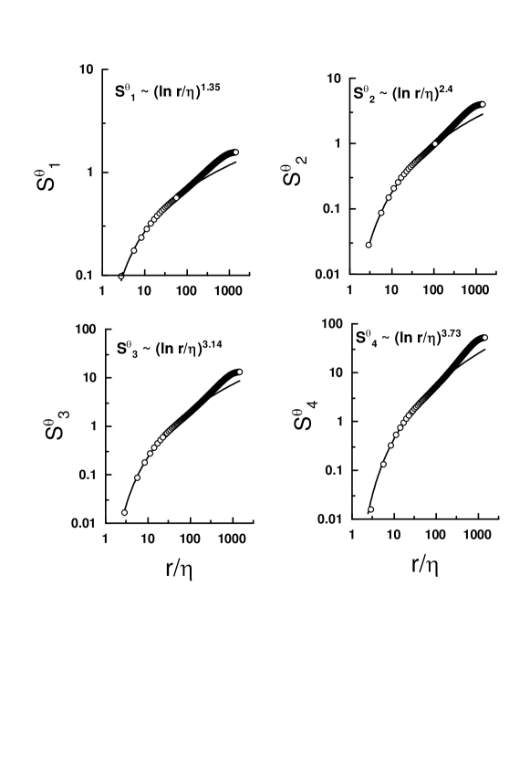
Figure 11: $S^{\theta}_{n}$ against $r/\eta$. The DNS data (circles) of homogeneous isotropic turbulence described in wg , Péclet number $P_{\lambda}=427$ and the Schmidt number is unity (i.e $P_{\lambda}=R_{\lambda}$). The solid curves are the best fit to the degenerate scaling (44).

The inertial-convective regime of a passive scalar field transport in isotropic turbulence for large Reynolds numbers is usually described using Obukhov-Corrsin theory my . This theory predicts scaling spectrum for the passive scalar ($\theta$) fluctuations with the scaling exponent equal to ”-5/3”

$$E^{\theta}(k)\sim\bar{\varepsilon}^{-1/3}\bar{\varepsilon}_{\theta}k^{-5/3}$$

where $\bar{\varepsilon}_{\theta}$ is the average value of dissipation rate of scalar variance, ${\varepsilon}_{\theta}$ (cf Eq. (9)). In the experiments, however, this regime is not usually observed (especially, for moderate Reynolds numbers and in turbulent shear flows). In the last case the experiments indicate a strong dependence of the passive scalar spectra on the Reynolds number (see, for instance, Refs. sreeni1 , warhaft and references therein). In the vein of the Section IV the dimensional considerations applied to the non-local asymptotic result in the power-law spectrum

$$E^{\theta}(k)\sim\frac{\bar{\varepsilon}_{\theta}}{s}~{}k^{-1}$$

(cf Eq. (10) and nl ,ldn ,vid ). Accordingly, both scaling regimes (34) and (35) can be corrected (for simplicity we restrict ourselves by the case when the Schmidt number is unity wg ). The first order correction is

$$E_{\theta}(k)\sim k^{-5/3}[\ln(k_{d}/k)]^{\gamma}$$

and

$$E^{\theta}(k)\sim k^{-1}[\ln(k_{d}/k)]^{\beta}$$

for the local and non-local regimes respectively ($\gamma$ and $\beta$ are dimensionless constants, different from those in Eqs. (11),(12) ).

One can estimate the second order structure function for the passive scalar fluctuations

$$S^{\theta}_{2}(r)=\langle|\Delta\theta|^{2}\rangle=\langle|\theta({\bf r}+{\bf x})-\theta({\bf r})|^{2}\rangle$$

as

$$S^{\theta}_{2}(r)\sim\int_{1/r}^{1/\eta}E^{\theta}(k)dk$$

(cf Eq. (13)). Then for $r<r_{c}$ using Eqs. (37) and (39) one obtains

$$S^{\theta}_{2}(r)\sim[\ln(r/\eta)]^{\zeta_{2}}$$

with $\zeta_{2}=\beta+1$ (cf Section IV).

Figure 10 shows $S^{\theta}_{2}$ against $r/\eta$ for the DNS data of homogeneous isotropic turbulence described in wg , Péclet number $P_{\lambda}=427$ and the Schmidt number is unity (i.e. $P_{\lambda}=R_{\lambda}$). The solid curve is the best fit to the degenerate scaling (40) (the dashed straight line indicates the Obukhov-Corrsin ordinary scaling my ,wg ).

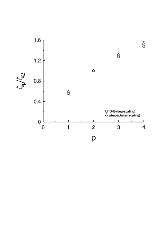
Figure 12: Exponents extracted from Fig. 11 (circles) and for the fully developed atmospheric turbulence (ordinary scaling in the inertial interval, triangles lov ).)

As in Section IV we can generalize (39) introducing an effective spectrum $E^{\theta}_{n}(k)$

$$S^{\theta}_{n}(r)=\langle|\Delta\theta|^{n}\rangle\sim\int_{1/r}^{1/\eta}E^{\theta}_{n}(k)dk$$

($E^{\theta}_{2}(k)\equiv E^{\theta}(k)$). Then using the dimensional considerations we obtain for the non-local regime

$$E^{\theta}_{n}(k)\sim\left(\frac{\bar{\varepsilon}_{\theta}}{s}\right)^{n/2}~{}k^{-1}$$

The first order correction is

$$E^{\theta}_{n}(k)\sim\left(\frac{\bar{\varepsilon}_{\theta}}{s}\right)^{n/2}~{}k^{-1}[\ln(k_{d}/k)]^{\beta_{n}}$$

Substituting (43) into (41) one obtains

$$S^{\theta}_{n}(r)\sim\left(\frac{\bar{\varepsilon}_{\theta}}{s}\right)^{n/2}~{}[\ln(r/\eta)]^{\zeta_{n}}$$

with $\zeta_{n}=\beta_{n}+1$.

Figure 11 shows $S^{\theta}_{n}$ against $r/\eta$ for the DNS data of homogeneous isotropic turbulence described in wg , Péclet number $P_{\lambda}=427$ and the Schmidt number is unity (i.e $P_{\lambda}=R_{\lambda}$). The solid curves are the best fit to the degenerate scaling (44).

One can readily expand the conclusions of the section V regarding Extended Self-Similarity on the case of passive scalar and we show effectiveness of this in figure 12. The data for degenerate scaling (circles) were taken from the degenerate scaling shown in Fig. 11 whereas the data for the ordinary scaling (triangles) were taken from a high Reynolds number atmospheric experiment lov .

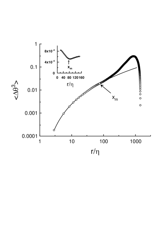
Figure 13: $\langle\Delta\theta^{3}\rangle$ against $r/\eta$. The DNS data (circles) of homogeneous isotropic turbulence described in wg , Péclet number $P_{\lambda}=427$ and the Schmidt number is unity (i.e $P_{\lambda}=R_{\lambda}$). The solid curve is the best fit to the degenerate scaling. The inset shows with high resolution the derivative of $\langle\Delta\theta^{3}\rangle$ in a vicinity of its minimum. The arrow indicates position of the generalized energy input rate maximum $x_{m}\simeq r_{c}$ calculated using $D_{LLL}$.

The overlapping phenomenon (Section VI) takes also place for the $S^{\theta}_{n}$ as for $S_{n}$. In $\langle\Delta\theta^{3}\rangle$ like in $D_{LLL}$ most positive contributions are canceled by negative ones and only the slight asymmetry of the $\Delta\theta$ probability density contributes to $\langle\Delta\theta^{3}\rangle$. However, similarly to $D_{LLL}$ this asymmetry has a fundamental nature. Therefore, one can expect that $\langle\Delta\theta^{3}\rangle$ also can be used in order to determine $r_{c}$. Moreover, since $\langle\Delta\theta^{3}\rangle$ as function of $r/\eta$ has a turnover point, as one can see in figure 13, the turnover point should indicate the point where the actual declination of the degenerate scaling fit from the data should begin. In the turnover point derivative of the function $\langle\Delta\theta^{3}\rangle$ has its minimum. In the inset to Fig. 13 we show with high resolution the derivative in a vicinity of its minimum. We also indicate with arrow the position of local maximum of the generalized energy input rate $x_{m}\simeq r_{c}$ calculated using $D_{LLL}$ for this case (cf Section VI).

One can see that the suggested perturbation theory with the degenerate scaling is an appropriate tool for description of data in the near-dissipation range. For modest Reynolds numbers the degenerate scaling applies to nearly the entire range of scales. Crossover between the degenerate and ordinary scaling provides an explanation to the Extended Self-Similarity. Interplay between local and non-local interactions can be considered as a possible hydrodynamics mechanisms of these phenomena.

- (1) R. Benzi, S. Ciliberto, R. Tripiccione, C. Baudet, F. Massaioloi, and S. Succi, Phys. Rev. E., 48: R29 (1993).
- (2) R. Benzi, L. Biferale, S. Ciliberto, M.V. Struglia and R. Tripiccione, Physica D 96: 162 (1996).
- (3) D. Sornette, Critical Phenomena in Natural Sciences (Springer, New York 2004).
- (4) L. Moriconi, A.L.C. Pereira, and P.A. Schulz, Phys. Rev. B 69: 45109 (2004).
- (5) K.G. Aivalis, K.R. Sreenivasan, Y. Tsuji, J.C. Kiewicki and C.A. Biltoft, Phys. Fluids, 14: 2439 (2002).
- (6) A. Bershadskii and K.R. Sreenivasan, Phys. Rev. Lett., 93: 064501 (2004).
- (7) A.S. Monin and A.M. Yaglom, Statistical Fluid Mechanics, Vol. 2, (MIT Press, Cambridge 1975)
- (8) K.R. Sreenivasan and R.A. Antonia, Annu. Rev. Fluid Mech. 29: 435 (1997)
- (9) M. Nelkin, Adv. Phys. 43: 143 (1994).
- (10) C. Meneveau, Phys. Rev. E 54: 3657 (1996).
- (11) T. Nakano, D. Fukayama, A. Bershadskii, and T. Gotoh, J. Phys. Soc. Japan, 71: 2148 (2002).
- (12) K.R. Sreenivasan and A. Bershadskii, Pramana, 64: 315 (2005).
- (13) J. Schumacher, K. R. Sreenivasan, and V. Yakhot, arXiv:nlin.CD/0604072
- (14) V. Yakhot, Physica D, 215 166 (2006).
- (15) K.R. Sreenivasan and A. Bershadskii, J. Fluid. Mech. 554: 477 (2006).
- (16) G.K. Batchelor, G.K. An Introduction to Fluid Dynamics (Cambridge University Press, Cambridge, 1970).
- (17) B.R. Pearson, P.-A. Krogstad and W. van de Water, Phys. Fluids 14: 1288 (2002)
- (18) T. Gotoh, D. Fukayama and T. Nakano, Phys. Fluids, 14: 1065 (2002)
- (19) H.S. Kang, S. Chester and C. Meneveau, J. Fluid. Mech., 480: 129 (2003).
- (20) B.B. Kadomtsev, Plasma Turbulence (Academic Press, New York, 1965).
- (21) S. Nazarenko and J.-P. Laval, J. Fluid Mech., 408: 301 (2000).
- (22) J-P. Laval, B. Dubrulle and S. Nazarenko, Phys. Fluids, 13: 1995 (2001).
- (23) K.R. Sreenivasan and B. Dhruva, Prog. Theor. Phys. Suppl. 130: 103 (1998)
- (24) E.A. Novikov, Sov. Phys. JETP, 20: 1290 (1965).
- (25) K.R. Sreenivasan, Phys. Fluids, 8: 189 (1996).
- (26) Z. Warhaft, Ann. Rev. Fluid Mach., 32: 203 (2000).
- (27) E. Villermaux, C. Innocenti and J. Duplat, Phys. Fluids, 13, 284 (2001).
- (28) T. Watanabe and T. Gotoh, New J. Phys. 6: Art. No. 40. (2004)
- (29) F. Schmidt, D. Schertzer, S. Lovejoy and Y. Brunet, Europhys. Lett. 34: 195 (1996).