Sawtooth disruptions and limit cycle oscillations

Abstract

A minimal (low-dimensional) dynamical model of the sawtooth oscillations is presented. It is assumed that the sawtooth is triggered by a thermal instability which causes the plasma temperature in the central part of the plasma to drop suddenly, leading to the sawtooth crash. It is shown that this model possesses an isolated limit cycle which exhibits relaxation oscillation, in the appropriate parameter regime, which is the typical characteristics of sawtooth oscillations. It is further shown that the invariant manifold of the model is actually the slow manifold of the relaxation oscillation.

1 Introduction

Sawtooth oscillations [1], commonly observed in current carrying, magnetically confined plasmas, are believed to be the result of resistive internal kink mode i.e. $(m=1,n=1)$ oscillation. These oscillations are characterized by a relatively slow rise of the electron temperature in the central region of the plasma column followed by a rapid drop (the crash). This is a typical nature of a stick-slip or relaxation oscillation [2], where the stress is slowly built up and then suddenly released after a certain threshold, observed in many other dynamical systems e.g. Portevin-Le Chatelier effect [3], a matter of interest in material science.

In this work, we propose a minimal (low-dimensional) dynamical model for sawtooth oscillation in tokamaks, based on a transport catastrophe due to a thermal instability [4]. Low-dimensional or low-order dynamical system i.e. a system of coupled ordinary differential equations, has several advantages over a detailed physical model of the actual system in the understanding of the global behaviour of the system. These models become powerful as they are supported by well developed mathematical theories which can be used to gain insight into the qualitative behaviour of the system such as bifurcation and stability [5]. Several examples of these models can be found in the context of understanding the behaviour of fusion plasmas ranging from the edge localized modes (ELM) [6] to plasma turbulence [7].

In spite of a great deal of experimental and theoretical research, the sawteeth in tokamaks continue to be a subject of exploration. For example, though numerical simulations [8] and some experimental results [9] suggest total reconnection within the safety factor $q=1$ surface during a sawtooth crash, there are also experimental evidences [10], which indicate that $q$ remains well below unity during a sawtooth cycle. Apparently, there have been several important contributions to the understanding of the sawtooth dynamics e.g. sawteeth with partial reconnection, based on turbulent transport [13]. A Taylor relaxation model of the sawteeth has also been considered by Gimblett and Hastie [14].

Here, we primarily focus on the dynamics of sawtooth oscillations based on a low-dimensional dynamical model. We rigorously prove that this dynamical model of the sawteeth based on thermal instability, besides capturing the important physical aspects, does exhibit well defined, isolated limit cycle oscillations, characteristics of self-excited relaxation phenomena like the sawteeth. Alternatively, several authors have proposed Hamiltonian models [15, 16, 17], which however can have infinite number of periodic solutions depending on the starting points of the evolution with the same set of physical parameters, which is rather inconsistent with the universal nature of sawteeth for similar experimental conditions. These models, despite having dissipation, possess a conserved quantity much like the Hamiltonian of a conjugate system.

In Section II, we formulate the minimal dynamical model. In Section III, we analyse the bifurcation and stability of the system, pointing out the existence of an isolated and unique limit cycle and its global stability. We complete this section by proving the uniqueness of the limit cycle where we demonstrate the existence of an algebraic equation for the limit cycle. Next, in Section IV, we address the issue of relaxation oscillation and explore the parameter regime where the limit cycle exhibits sawtooth-like oscillations. In Section V, with the help of a renormalization group method, we prove that the invariant manifold of the dynamical system is indeed the slow manifold of the relaxation oscillation. In the Appendix, we outline the Hamiltonian approach to this dynamical model.

2 Dynamical modeling of sawtooth oscillations

Typical sawtooth oscillations in small tokamaks $(R_{0}=1\,{\rm m})$ exhibit linear growth of central temperature with few milliseconds of duration and rapid crash time of $\sim$ several microseconds, in the Ohmic heating phase [18, 19, 10]. Although there are several other exotic cases viz. giant and monster sawteeth [11, 12], we shall limit our discussion to the simpler type of sawteeth with a linear rise of the electron temperature. The dynamical system, controlling the sawtooth oscillations of the central electron temperature, then can be written as [4, 15, 20]

$$\frac{3}{2}n\frac{\partial T_{e}}{\partial t} = E_{\parallel}^{2}\sigma_{\parallel}-\nu_{L}(A,T_{e})nT_{e,}$$ (1)

$$\frac{\partial A}{\partial t} = \gamma(T_{e})A,$$ (2)

where $T_{e}$ is the central electron temperature expressed in energy units, $A$ is the amplitude of the oscillation, $\nu_{L}(A,T_{e})$ is the rate of temperature redistribution, and $\gamma(T_{e})$ is the growth rate of the relevant mode. The collisional parallel conductivity $\sigma_{\parallel}\propto T_{e}^{3/2}$. In the above equations, the particle density $n$ remains nearly constant during the sawtooth cycle, which is consistent with experimental observations. We further note that in the cases of sawtooth oscillations, we are going to consider, the classical diffusion time [21] for the plasma current within the $q\leq 1$ volume, $\tau_{J}=(r_{1}/d_{e})^{2}/\nu_{ei}$ (where $r_{1}$ is the radius of the $q=1$ surface, $d_{e}$ is the plasma skin depth, and $\nu_{ei}$ is the electron-ion collision frequency), is one order of magnitude higher than the sawtooth repetition time. For example, in the Alcator C-Mod (MIT) machine, typically, $\tau_{J}\sim 80$-$400\,{\textrm{msec}}$ for Ohmic regimes [22], whereas the sawtooth period (crash time being negligibly smaller than the period) $\tau_{{\textrm{st}}}\sim 4\,{\textrm{msec}}$. Therefore it can be safely assumed that the current redistribution does not play any significant role and the corresponding $E_{\parallel}$ remains constant. We further assume that the pressure redistribution parameter $\nu_{L}(A,T_{e})$ can be expressed with simple power laws i.e. $\nu_{L}(A,T_{e})\propto T_{e}^{\alpha}A^{\sigma}$, where $\alpha$ and $\sigma$ are arbitrary constants.

With these considerations, we note that the second term in Eq.(1) is responsible for the sawtooth crash. However, in absence of this term the general solution of Eq.(1) is explosive. In particular, it should include a loss term, which takes into account all other losses e.g. radiation loss, electron thermal diffusion [23], and neoclassical loss [24] etc. With a diffusive loss term, Eq.(1) can be rewritten as

$$\frac{3}{2}n\frac{\partial T_{e}}{\partial t}=E_{\parallel}^{2}\sigma_{\parallel}-\nu_{L}^{0}nT_{e}^{\alpha}A^{\sigma}-\frac{3}{2}\frac{nT_{e}}{\tau_{E}},$$ (3)

where $\tau_{E}$ is the overall plasma energy confinement time inside the $q=1$ surface and $\nu_{L}^{0}$ is a proportionality constant. In fact, the presence of the diffusive loss term can be understood from the usual pressure gradient equation without taking into account the instability which causes the ejection of plasma energy due to sawtooth crashes,

$$\frac{\partial p}{\partial t}=S_{{\rm Oh}}+\nabla\cdot\chi_{\perp}\nabla p,$$ (4)

where $p\sim nT_{e}$ is the plasma pressure, $S_{{\rm Oh}}$ is the Ohmic source term i.e. the heating power density per unit volume, and $\chi_{\perp}$ is the plasma thermal conductivity perpendicular to the magnetic field. Attributing all other losses to this diffusive term, we can write [26]

$$(\nabla\cdot\chi_{\perp}\nabla)\sim-\tau_{E}^{-1}.$$ (5)

Considering the fact that the plasma confinement time $\tau_{E}$ scales as $\sim a^{2}/\chi_{D}$, $a$ being the minor radius of the torus and $\chi_{D}$, a diffusion coefficient which obeys Bohm-like diffusion, i.e. $\chi_{D}=\rho_{i}\chi_{B}/a$, where $\chi_{B}=T_{e}/16eB$, $\rho_{i}$ is the ion gyro-radius, and $B$ is the ambient toroidal magnetic filed. Assuming that $T_{i}\approx T_{e}$, the last term in Eq.(3) can be shown to scale as $\sim T_{e}^{5/2}$ and Eq.(3) becomes

$$\frac{3}{2}n\frac{\partial T_{e}}{\partial t}=E_{\parallel}^{2}\sigma_{\parallel}-\nu_{L}^{0}nT_{e}^{\alpha}A^{\sigma}-\beta nT_{e}^{5/2},$$ (6)

where $\beta$ is a constant of proportionality. Note that the above relation of electron temperature evolution closely resembles the corresponding equation of sawtooth model by Kubota et. al. [27], based on transport bifurcation.

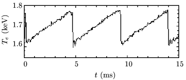
Figure 1: A typical sawtooth cycle in the Alcator C-Mod (MIT) machine (Shot No. #960130034 [22]).

We now consider Eq.(2) which controls the amplitude evolution of the mode. During one sawtooth cycle of the profile shown in Fig.1, observed in the Alcator C-Mod machine at MIT [22]. Since the sawtooth crash time is much smaller than the sawtooth growth time, the mode amplitude can be considered to have a ‘spike-like’ behavior. In the limiting case, the spike becomes a singularity and can be represented by a $\delta$ function,

$$A\sim\delta(t-t_{0}),$$ (7)

centered around $t=t_{0}$. The corresponding relation for $T_{e}$ can be found out from Eq.(1) as

$$T_{e}=t-\xi H(t-t_{0}),$$ (8)

where $\xi$ is some constant and $H(t)$ is the Heaviside step function. This behavior of $T_{e}$ shows a perfect sawtooth with a crash occurring at $t=t_{0}$ and a discontinuity in $T_{e}$. In practice, the ‘spike-like’ behavior of amplitude $A$ can be approximated by an exponential function,

$$A\sim\exp\bigl{[}-\mu(t-t_{0})^{2}\bigr{]},$$ (9)

where $\mu$ is some large positive number. The corresponding $T_{e}$ is

$$T_{e}\sim t-\xi_{1}\left\{\sqrt{{2\mu}}(t-t_{0})\right\}+\xi_{2}.$$ (10)

The related differential equation in $A$ is, therefore,

$$\frac{dA}{dt}\simeq-2\mu(t-t_{0})A.$$ (11)

The coefficient of $A$ on the right hand side of the above equation can be viewed as $\gamma(T_{e}(t))$. So the complete set of dynamical equations can now be written as

$$\frac{3}{2}n\frac{dT_{e}}{dt} = E_{\parallel}^{2}\sigma_{\parallel}-\nu_{L}^{0}nT_{e}^{\alpha}A^{\sigma}-\beta nT_{e}^{5/2},$$ (12)

$$\frac{dA}{dt} = \gamma_{0}\left(\frac{T_{e}}{T_{s}}-1\right)A,$$ (13)

where $T_{s}$ is the threshold temperature for the onset of the relevant instability. We would like to emphasize that the model proposed by Haas and Thyagaraja [24], based on turbulent transport essentially reduces to the above equations when the neoclassical losses are discarded (they have a exclusive term to take care of the neoclassical loss).

At this point, we would like to note that in reality, sawtooth oscillations in magnetically confined plasmas are result of evolution of a ‘driven-dissipative’ system. During a sawtooth cycle, the plasma is heated by the current through Ohmic dissipation which is essentially lost to the environment after the plasma breakdown or the sawtooth crash. The sawtooth is repeated as the plasma current continues to dissipate energy into the plasma. Here, the plasma current is the driving mechanism of the sawtooth oscillation through which, the energy is being continuously dissipated. However, there is no driving source in Eq.(12) and the oscillations represented by Eqs.(12-13) appears to be self-sustaining i.e. a “self heating – dissipating – feedback – heating” cycle with a positive and negative damping mechanism through the terms $\left(E_{\parallel}^{2}\sigma_{\parallel}-\beta nT_{e}^{5/2}\right)$. The justification for Eq.(12) comes from the fact that we are looking only at the power balance equation for the confined plasma [25], not at the full burn-cycle of the plasma confinement. So, as far as the plasma power balance is concerned, we assume that there is a perpetual source of energy in the form of the plasma current provided externally through the loop voltage, which is the driving mechanism and an infinite sink which drains away the energy dissipated through the sawtooth crash. As the whole cycle repeats, the power balance equation becomes self-sustaining.

We further note that during the sawtooth ramp phase, there is a definite change in the magnetic configuration, which rearranges itself after the sawtooth crash either through a partial or complete reconnection [23]. As this magnetic reorientation causes the electron temperature to drop during the sawtooth crash, we have dynamically modeled this event by the second term $\left(\nu_{L}^{0}nT_{e}^{\alpha}A^{\sigma}\right)$, in Eq.(12).

3 Stability and bifurcation — limit cycle oscillation

In this section, we examine the possibility of existence of periodic orbits of Eqs.(12) and (13), in particular existence of any limit set. This is to be viewed in contrast to the Hamiltonian formalism (see Appendix), which always admits periodic solutions, though the solutions are not unique.

We begin by expressing these dynamical equations in a generic dimensionless form. The electron temperature $T_{e}$ is normalized by the threshold temperature $T_{s}$ and define $x=T_{e}/T_{s}$. We further define the other dimensionless quantities as

$$\frac{2}{3}\frac{\nu_{L}^{0}T_{s}^{\alpha-1}}{S_{{\rm Oh}}}A^{\sigma}=y,\qquad\frac{2}{3}\frac{\beta}{S_{{\rm Oh}}}T_{s}^{3/2}=a.$$ (14)

The quantity $y$ denotes the normalized amplitude of the mode and the quantity $S_{{\rm Oh}}$ is the Ohmic source term corresponding to the threshold temperature $T_{s}$,

$$S_{{\rm Oh}}=\frac{2}{3}\frac{E_{\parallel}^{2}\sigma_{s\parallel}}{nT_{s}},$$ (15)

the quantity $\sigma_{s\parallel}$ being the collisional conductivity at $T_{e}=T_{s}$. With these definitions, the set of Eqs.(12) and (13) can be written in a generic form as

$$\dot{x} = x^{(3/2)}(1-ax)-x^{\alpha}y,$$ (16)

$$\dot{y} = \rho(x-1)y,$$ (17)

where $\rho=\sigma\gamma_{0}/S_{{\rm Oh}}$. Note that in writing these equations we have re-scaled the time as $t\rightarrow S_{{\rm Oh}}t$. As we shall see shortly that the constant $a<1$ while $\rho$ which is related to the growth rate can be quite large i.e. $\gg 1$. The dots represent the derivatives with respect to the rescaled time $t$.

Figure 2: Phase portrait of Eqs.(16) and (17). The arrows denote the direction of flow.

In order to examine the bifurcation diagram of Eqs.(16) and (17) and existence of limit cycle oscillation, it is instructive to construct a phase portrait of the equations, which is shown in Fig.2. The arrows on the curves show the direction of time. As can be seen, there are three fixed points, ‘A’, ‘B’, and ‘C’ located at $(x,y)=(0,0)$, $(1,1-a)$, and $(1/a,0)$, respectively. Point ‘A’ at the origin is a non-isolated fixed point. Point ‘C’ is a saddle point. The only fixed point of interest is the point ‘B’ which is either a stable or unstable point depending on values of $\alpha$ and $a$. We are also interested in this fixed point as this is the only point which is in the positive quadrant as the variables $x$ and $y$ may take only positive values. In what follows, we shall show that surrounding the fixed point ‘B’, we can construct a positively invariant region [28] lying entirely in the first quadrant.

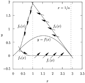
Figure 3: A positively invariant region for Eqs.(16) and (17).

3.1 Limit cycle oscillation

Consider now, a set of curves $f_{i}(x)$ given by the equations

$$f_{1}(x) = 0,$$ (18)

$$f_{2}(x) = \mathcal{C}\left(\frac{1}{a}-x\right),$$ (19)

$$f_{3}(x) = x\left[\mathcal{C}\left(\frac{1}{a}-1\right)+\delta\right]-\delta,$$ (20)

$$f_{4}(x) = \mathcal{D}(1-x)^{2\mu+1},$$ (21)

where ${\mathcal{\mathcal{C}}}$ can be a large positive number, $\delta$ is a small positive number, and $\mathcal{D}$ and $\mu$ are positive arbitrary constants. The nullclines of the Eqs.(16) and (17) are given by the equations

$$x = 1,$$ (22)

$$y = x^{3/2-\alpha}(1-ax)=f(x).$$ (23)

If we now span a region (see Fig.3) described by the set of curves $f_{i}(x)$s through the points $(1,0)$, $(1/a,0)$, $(1,\mathcal{C}(1/a-1))$, and $(x^{\prime},y^{\prime})$ — the points of intersection of the curves $f_{i}(x)$ and $f(x)$, $(x^{\prime},y^{\prime})$ being the common point of intersection of $f_{3,4}(x)$ and $y=f(x)$, it can be shown by comparing the slopes of the curves $f_{i}(x)$s with that of the orbit described by Eqs.(16) and (17), that the flow of the orbit of Eqs.(16) and (17) always crosses into the closed region, anticlockwise [28]. Thus the flow of the orbit of Eqs(16) and (17) is always bounded and the closed region in Fig.3 constitutes a positively invariant region for Eqs.(16) and (17). An example set of parameters for this positively invariant region are $a=0.34$, $\alpha=1/2$, ${\mathcal{\mathcal{C}}}=1$, $\mu=1$, $\mathcal{D}=0.923$, and $\delta=1/2$, the point $(x^{\prime},y^{\prime})=(0.322,0.287)$.

What needs to shown now is the fact that for the permitted parameter regime, the fixed point ‘B’ is an unstable point. We linearize the set of equations (16) and (17) around the fixed point ‘B’ $=(1,1-a)$ and the eigenvalues of the linear part of these equations at $(1,1-a)$ are

$$\lambda_{1,2}=\frac{1}{2}\left(\tau\pm\sqrt{{\tau^{2}-4\Delta}}\right),$$ (24)

where

$$\tau = \frac{3}{2}-\frac{5}{2}a-\alpha(1-a),$$ (25)

$$\Delta = \rho(1-a),$$ (26)

and the stability of the equilibrium point ‘B’ depends on the values of $\tau$ and $\Delta$. As $\rho\gg 1$ and $a<1$, we can find that the point ‘B’ is an unstable spiral, if

$$a<\left(\frac{3/2-\alpha}{5/2-\alpha}\right)=a_{c},\>\alpha<\frac{3}{2}=\alpha_{c}.$$ (27)

The existence of the limit cycle is now evident according to the Poincaré-Bendixson condition [2].

The point ‘B’ also becomes unstable for $\alpha>5/2$ provided $a>1$, however the latter is excluded by our physical conditions. As the growth rate of the instability should be large enough to cause a sawtooth crash, $\rho\gg 1$. This also ensures that the fixed point ‘B’ is an unstable spiral. Also, we observe that as $a\rightarrow 1$, $\alpha\rightarrow\infty$. In fact, at $a=a_{c}$ (for a certain $\alpha<\alpha_{c}$), a supercritical Hopf bifurcation occurs [2, 28]. The bifurcation surface for Eqs.(16) and (17) is shown in Fig.4. Note the steepening of the surface $f(x,\alpha)$, given by Eq.(23), as $\alpha\rightarrow 3/2$ and the disappearance of the fixed point ‘A’$=(0,0)$ at the bifurcation point.

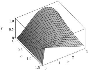
Figure 4: Bifurcation diagram for the set of equations (16) and (17).

In Fig.5, we show the limit cycle for a set of parameters $\alpha=1$, $a=0.33$, and $\rho=1$. At the birth of the limit cycle after the supercritical Hopf bifurcation, the period of the limit cycle is given by the Hopf period,

$$\tau_{{\rm Hopf}}=\frac{4\pi}{\sqrt{{4\Delta-\tau^{2}}}}\approx\frac{2\pi}{\sqrt{{\rho(1-a)}}}.$$ (28)

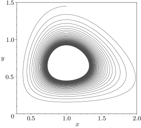
Figure 5: The limit cycle for Eqs.(16) and (17) subject to condition (27).

3.2 Local and global stability of the limit cycle

Though the phenomena of sawtooth oscillations in magnetically confined plasmas suggests existence of a ‘driven-dissipation’ type limit cycle oscillation, experimentally observed sawtooth oscillations are, in general, perturbed by local irregularities and fluctuations. As limit cycles are usually characterised by a flow field which converges to the cycle everywhere, it is important to classify the orbital stability of the limit cycle in order to emphasize its response to noise.

The classical method for studying orbital stability of limit cycles involves eigenvalues of the Poincaré map [29]. Several other variants also exist in literature, for studying local stability [30, 31], among which the most common one is the theory of Floquet multipliers or the monodromy matrix method, where one follows the short-time evolution of a small perturbation $\delta\bm{x}$ along the limit cycle. Another widely applicable method is associated with the direction of slowest decay [32]. Here, we employ a method based on applying a small perturbation $\delta\bm{x}(t)$ to the non-stationary reference solution i.e. limit cycle of the flow $\bm{x}_{0}(t)$ and following the directions tangential and transverse to the flow along the perturbed trajectory $\bm{x}(t)=\bm{x}_{0}(t)+\delta\bm{x}(t)$ [33].

Consider the dynamical system

$$\frac{d}{dt}\bm{x}(t)=\bm{F}[\bm{x}(t)].$$ (29)

If the perturbations $\delta\bm{x}(t)$ are small enough, the evolution can be linearised

$$\frac{d}{dt}\delta\bm{x}=\bm{A}\,\delta\bm{x},\qquad A_{ij}=\left(\frac{\partial\bm{F}_{i}}{\partial x_{j}}\right)_{\bm{x}_{0}(t)}.$$ (30)

The linearised system (30) is transformed from the fixed basis $\bm{x}$ to the rotating, orthogonal basis $\bm{x}^{\prime}$ through a unitary rotation matrix $\bm{U}$, $\delta\bm{x}^{\prime}=\bm{U}\,\delta\bm{x},\delta\bm{x}=\bm{U}^{-1}\,\delta\bm{x}^{\prime}$, so that the linearised system (30) becomes

$$\frac{d}{dt}\delta\bm{x}^{\prime}=\bm{B}\,\delta\bm{x}^{\prime},$$ (31)

where

$$\bm{B}=\bm{U}\bm{A}\bm{U}^{-1}+\frac{d\bm{U}}{dt}\bm{U}^{-1}.$$ (32)

is the stability matrix.

For a two-variable system like ours [Eqs.(16-17)],

$$\dot{x} = f(x,y),$$ (33)

$$\dot{y} = g(x,y),$$ (34)

the stability matrix $\bm{B}$ is given by

$$\bm{B}=\left(\begin{array}[]{cc}\lambda_{tt}&\lambda_{tn}\\ \lambda_{nt}&\lambda_{nn}\end{array}\right),$$ (35)

where

$$\lambda_{tt} = [f^{2}f_{x}+g^{2}g_{y}+fg(f_{y}+g_{x})]/(f^{2}+g^{2}),$$ (36)

$$\lambda_{tn} = [(g^{2}-f^{2})(f_{y}+g_{x})+2fg(f_{x}-g_{y})]/(f^{2}+g^{2}),$$ (37)

$$\lambda_{nt} = 0,$$ (38)

$$\lambda_{nn} = [f^{2}g_{y}+g^{2}f_{x}-fg(f_{y}+g_{x})]/(f^{2}+g^{2}).$$ (39)

are the rates of convergence of the flow from the perturbed trajectory into the limit cycle. Parameter $\lambda_{nn}$ represents the rate of convergence normal to the flow and $\lambda_{tt}$ represents convergence tangential to the flow, which essentially averages to zero over a full cycle. The tangential and normal perturbations are only partially coupled as $\lambda_{nt}=0$, which means that a tangential perturbation remains tangential whereas a normal perturbation couples to the tangential perturbations (nonzero $\lambda_{tn}$). So a perturbation is unstable or stable depending on whether $\lambda_{ij}$ is positive or negative. The global stability measures can be found out from the Lyapunov exponent, which can be obtained by phase averaging the $\lambda_{ij}$s over an orbit with period $T$ [33],

$$\Lambda_{ij}=\frac{1}{T}\oint\lambda_{ij}(\phi)\,d\phi,$$ (40)

corresponding to a particular perturbation. A negative $\Lambda$ would imply global stability. In practice we use a discretised version of Eq.(40),

$$\Lambda_{ij}=\frac{1}{m}\sum_{k=1}^{m}\lambda_{ij}(t_{0}+k\,\Delta t),\qquad m\,\Delta t=T.$$ (41)

In Fig.6, we show the stability properties of the limit cycle oscillation of Eqs.(16-17) for a set of parameters $\alpha=1,a=0.33$, and $\rho=100$, which produces a relaxation type oscillation (see Fig.8). As one can see that the limit cycle consists of unstable and stable parts corresponding to the normal perturbations. The limit cycle is globally stable as indicated by the global stability parameter, the Lyapunov exponent $\Lambda_{nn}=-0.00431$. The plot of $\Lambda_{tt}$ shows the tangential stability which is essentially due to acceleration and deceleration of the flow showing a relaxation mechanism. As expected, the average $\Lambda_{tt}\approx 0$ within the computational accuracy. The coupling matrix element $\lambda_{tn}$ represents the effect of perpendicular perturbation on the oscillator phase. During $\lambda_{tn}>0$, the perpendicular perturbation leads to advancement of the phase of the oscillator and $\lambda_{tn}<0$ indicates a phase delay.

Figure 6: Local and global stability of the limit cycle of Eqs.(16-17) away from the Hopf bifurcation point. Clockwise from top, in the first plot, the unstable (dotted) and stable (solid) parts of the limit cycle in the phase plane are shown. The variations of $\lambda_{nn},\lambda_{tn}$, and $\lambda_{tt}$ are shown over one phase of the limit cycle in the second, third, and fourth plots.

3.3 Equation of the limit cycle

In this subsection, we find out an equation for the limit cycle enclosing the critical point ‘B’ in terms of a series expansion. Here, we employ a method due to Giacomini and Viano [34], which is based on the fact that if we consider the partial differential equation

$$P\frac{\partial V}{\partial x}+Q\frac{\partial V}{\partial y}=\left(\frac{\partial P}{\partial x}+\frac{\partial Q}{\partial x}\right)V,$$ (42)

corresponding to the two-dimensional dynamical system

$$\dot{x}=P(x,y),\qquad\dot{y}=Q(x,y),$$ (43)

there exists a unique convergent power series solution of Eq.(42) in some region $\mathfrak{R}$ containing a non-degenerate critical point $P_{0}$ of node or focus (spiral) type and that this solution satisfies

$$V(x,y)=0$$ (44)

on any limit cycle contained in $\mathfrak{R}$ which encloses $P_{0}$. In our case, the equations (16) and (17) have an isolated limit cycle enclosing the critical point located at $(1,1-a)$. We have already seen that subject to the conditions (27), the equilibrium point ‘B’ is an unstable spiral. Therefore, there exists a unique series solution of Eq.(42).

As the cases, where an explicit series solution can be calculated analytically, are limited to polynomial forms for the functions $P(x,y)$ and $Q(x,y)$, we write the Eqs.(16,17) with a transformation of variable $x\rightarrow x^{2}$, so that our system of dynamical equations become

$$\dot{x} = \frac{1}{2}x^{2}(1-ax^{2})-\frac{1}{2}x^{2\alpha-1}y,$$ (45)

$$\dot{y} = \rho(x^{2}-1)y.$$ (46)

Without loss of any generality, the constant $\alpha$ can be set to unity, for which, the right hand sides of Eq.(45,46) become polynomials in $x$ and $y$. Following Giacomini and Viano [34], we now look for a power series

$$V(x,y)=\sum_{n=0}^{\infty}v_{n}(x,y),$$ (47)

where $v_{n}(x,y)$ is a homogeneous polynomial of degree $n$,

$$v_{n}(x,y)=\sum_{k=0}^{n}c_{n-k,k}x^{n-k}y^{k}.$$ (48)

In practice, we work on the truncated sum

$$V(x,y)=\sum_{n=0}^{N}v_{n}(x,y),$$ (49)

at order $N$ and try to solve for the coefficients $c_{n-k,k}$ from set of simultaneous equations generated from partial derivatives of Eq.(42) evaluated at the critical point $P_{0}=(1,1-a)$. The equation of the limit cycle is thus given by

Table 1: The coefficients $c_{n-k,k}$ for order $N=8$.

$c_{8,0}$	$1.0$			$c_{4,1}$	$84.977$			$c_{5,3}$	$-2.945$			$c_{3,5}$	$0.037$
$c_{7,0}$	$-6.724$			$c_{3,1}$	$-89.203$			$c_{4,3}$	$17.662$			$c_{2,5}$	$-0.494$
$c_{6,0}$	$19.626$			$c_{2,1}$	$56.673$			$c_{3,3}$	$-50.909$			$c_{1,5}$	$-5.958$
$c_{5,0}$	$-32.122$			$c_{1,1}$	$-16.609$			$c_{2,3}$	$60.445$			$c_{0,5}$	$-11.421$
$c_{4,0}$	$31.508$			$c_{6,2}$	$-1.691$			$c_{1,3}$	$-28.992$			$c_{2,6}$	$0.003$
$c_{3,0}$	$-17.578$			$c_{5,2}$	$12.896$			$c_{0,3}$	$-5.502$			$c_{1,6}$	$3.010$
$c_{2,0}$	$4.296$			$c_{4,2}$	$-43.927$			$c_{4,4}$	$-1.795$			$c_{0,6}$	$8.242$
$c_{1,0}$	$0.0$			$c_{3,2}$	$90.659$			$c_{3,4}$	$10.090$			$c_{1,7}$	$-0.550$
$c_{7,1}$	$-2.723$			$c_{2,2}$	$-96.759$			$c_{2,4}$	$-13.801$			$c_{0,7}$	$-3.522$
$c_{6,1}$	$17.608$			$c_{1,2}$	$44.352$			$c_{1,4}$	$12.472$			$c_{0,8}$	$0.658$
$c_{5,1}$	$-51.146$			$c_{0,2}$	$-2.460$			$c_{0,4}$	$10.162$

$$V(P_{0})=0.$$ (50)

For a set of parameters $\alpha=1$, $a=0.33$, and $\rho=1$, satisfying conditions (27), we calculate the coefficients $c_{n-k,k}$ with the help of the computer algebra system of Waterloo Maple [35] and find that a close curve fairly coinciding the numerically calculated limit cycle exists for an order as low as $N=8$. The corresponding curves of the the limit cycle are shown in Fig.7. Note that the value of $\rho=1$ does not necessarily produce a sawtooth, we however have chosen this value so as to find a close curve for $V(x,y)$ at the lowest possible order. The corresponding coefficients $c_{n-k,k}$ are tabulated in Table.1.

Figure 7: The limit cycle for Eqs.(32) and (33) as determined by the Eq.(37) (open circles) and numerically calculated one (solid).

For the sake of completeness, we review the equivalent Hamiltonian approximation of Eqs.(16) and (17), in the Appendix.

4 Relaxation oscillation and sawtooth disruptions

Relaxation oscillations are characterized by two very different time scales. As we can see from the phase portrait of Eqs.(16,17) in Fig.2, relaxation oscillation, if any, must be away from the Hopf bifurcation point i.e. $a=a_{c}$. So, we must push the system toward the boundary of the invariant region, defined by the equilibrium points ‘A’ and ‘C’, around the bifurcation point $(1,1-a)$. At the same time, it must be noted that far away from the bifurcation point i.e. for $a\ll a_{c}$, the orbit of the limit cycle will be swept away in the flow around the saddle point ‘C’.

A sawtooth trigger is caused by a sudden increase in a fast variable ($y$), as have already been pointed out in Sec.II, which remains almost close to zero for the rest of the sawtooth cycle. This ensures an almost linear rise of the sawtooth i.e. in the slow variable, the variable $x$, in our case. As shown in Fig.8, Eqs.(16,17) do indeed exhibit relaxation oscillations of sawtooth-type for an appropriate set of parameters.

Figure 8: Limit cycle, relaxation oscillation (sawtooth) of Eqs.(16) and (17). The parameters in this particular case are $\alpha=1$, $a=0.33$, and $\rho=100$.

The phase diagram of the corresponding limit cycle is shown Fig.8.

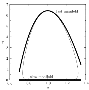
Figure 9: The phase diagram of the limit cycle (the thin closed curve) corresponding to the sawtooth oscillations shown in Fig.8. The fast and slow manifolds are shown in thick lines.

As expected the fast variable $y$ remains nearly zero for most of the time except for a vary short time, when it attains very high value, which causes the sawtooth crash.

The physical mechanism of this relaxation oscillation can be understood in terms of similar oscillations in model sandpile [36]. The corresponding variable in case of a sandpile is $\phi(x)$, the height of the pile at a position $x$. When sand is continuously added at the top of the pile, an instability occurs when the local slope of the pile becomes too large ($\nabla\phi$ greater than a critical value), causing an avalanche, which consists of rearrangements on the surface of the pile. In case of sawtooth oscillation, energy from the source flows at the rate $\sim x^{3/2-\alpha}$ [see Eq.(16-17)], causing the temperature to rise steadily, which then triggers an ‘avalanche’ after the temperature rises above a critical value.

4.1 The slow and fast manifolds

On the limit cycle, if we start from a point $x<1$ on the slow manifold (see Fig.9), the damping term in Eq.(16) i.e. $(x^{\alpha}y)$ remains very small as $y\approx 0$. As the constant $a<1$, $dx/dt$ remains positive and the slow variable $x$ increases in time. At the same time $dy/dt<0$ and $y$ further decreases as long as $x<1$. However as $x$ increases beyond unity, $dy/dt$ becomes positive and $y$ increases as $\sim\exp(t^{2})$, which causes the damping term in Eq.(16) to dominate over the growth term, triggering a crash. As soon as $x$ again falls below unity, $y$ rapidly drops [see Eq.(17)] and the whole cycle repeats. We expect that in the parameter region where this relaxation oscillations occur, the sawtooth growth time ($\tau_{{\rm st}}$) should be independent of the growth rate of the instability $\rho\gg 1$, whereas, the sawtooth crash time ($\tau_{{\rm c}}$) should be $\propto\rho^{-1}$.

To examine further, we note that on the slow manifold we can change the scale by introducing a small quantity $\epsilon$ which defines the fast time scale $t^{\prime}=t/\epsilon$. As the growth rate $\rho$ can be large and $y\approx 0$ on the slow manifold, rescaling them as

$$y=\epsilon\eta,\qquad\rho=\delta/\epsilon,\$$ (51)

we can write Eqs.(16,17) as

$$\dot{x} = x^{3/2}(1-ax)-\epsilon x^{\alpha}\eta,$$ (52)

$$\epsilon\dot{y} = \delta(x-1)\eta.$$ (53)

Taking the limit $\epsilon\rightarrow 0$, we obtain the slow manifold as

$$y = 0,$$ (54)

$$\dot{x} = x^{3/2}(1-ax),$$ (55)

so that the sawtooth period is essentially given by the time that the variable spends on the slow manifold,

$$\tau_{{\rm st}}\simeq\int_{x_{1}}^{x_{2}}\frac{dx}{x^{3/2}(1-ax)},$$ (56)

where $x_{1,2}$ are the points of intersection of the limit cycle with the nullcline $y=f(x)$ [see Eq.(23)]. As the drop in electron temperature i.e. $\Delta T_{e}\ll 1$ during a sawtooth crash, so is the drop in the corresponding dynamical variable $\Delta x$ and hence the amplitude of the sawtooth oscillation. Expanding Eq.(56) around the mean value of $x=1$, we can further estimate the sawtooth period in terms of its amplitude,

$$\tau_{{\rm st}}\sim(1-a)\Delta x.$$ (57)

On the fast manifold, as $y$ can attain large values, scaling $y$ as $\eta/\epsilon$ and time $t$ as $t^{\prime}\epsilon$, we have from Eqs.(16,17),

$$x^{\prime} = \epsilon x^{3/2}(1-ax)-x^{\alpha}\eta,$$ (58)

$$\eta^{\prime} = \delta(x-1)\eta,$$ (59)

where the $(^{\prime})$ denotes derivatives with respect to the fast time scale $t^{\prime}$. We obtain the fast manifold by letting $\epsilon\rightarrow 0$,

$$\dot{x} = -x^{\alpha}y,$$ (60)

$$\dot{y} = \rho(x-1)y,$$ (61)

which is essentially given by

$$y=\rho(\ln x-x+1)+y_{m},$$ (62)

for $\alpha=1$, $y_{m}$ being the maximum value of $y$ on the fast manifold which occurs at $x=1$. Both these manifolds are shown in Fig.9. The sawtooth crash time $\tau_{{\rm c}}$ can be approximately estimated from Eq.(59) and (61),

$$\tau_{{\rm c}}\simeq\int_{x_{2}}^{x_{1}}\frac{dx}{x[\rho(\ln x-x+1)+y_{m}]}.$$ (63)

As expected, in the parameter space of relaxation oscillation ($\rho\gg 1$), the sawtooth period is essentially independent of the growth rate $\rho$ while the crash time is inversely proportionate to it (see Fig.10). Note that with the index $p=0.5$, the total repetition time of the sawtooth $\tau=\tau_{{\rm st}}+\tau_{{\rm c}}$ closely follows the Hopf period as given by Eq.(28) when the oscillations remain purely sinusoidal for $\rho\sim 1$.

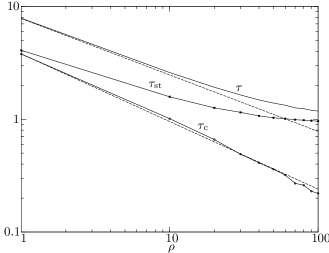
Figure 10: As $\rho$ becomes $\gg 1$, the sawtooth period $\tau_{{\rm st}}$ becomes independent of $\rho$. The crash time $\tau_{{\rm c}}$ however remains inversely proportionate to $\rho$, $\tau_{{\rm c}}\propto\rho^{-p}$. The dotted lines are the fitted curves for $\tau_{{\rm c}}$ and $\tau=\tau_{{\rm st}}+\tau_{{\rm c}}$ with the index $p=0.6$ and $0.5$, respectively.

4.2 Simulations of sawteeth

In Fig.11, we show the reproduction two sets of sawtooth oscillations from the Alcator C-Mod tokamak at MIT [22], which has an effective major and minor radius of $0.68\,{\rm m}$ and $0.22\,{\rm m}$. For the two experimental shots, (a) Shot No. #960130034 and (b) #960127012, the threshold temperatures $T_{s}$ are taken to be the average temperatures of the sawteeth, which are, $1.7$ and $1.4\,{\rm keV}$. The sawtooth time periods are respectively 4.63 and 3.6 milliseconds. The constant applied electric field is given by $E_{\parallel}=0.291$ and $0.352\,{\rm volt/m}$ which correspond to the Ohmic source term $S_{{\rm Oh}}\simeq 83.08$ and $62.09\,{\rm s^{-1}}$ for the value of Coulomb logarithm $\ln\Lambda\simeq 17$. The parallel plasma conductivity corresponding to the threshold temperature $T_{s}$ is given by

$$\sigma_{s\parallel}=9.71\times 10^{3}Z_{{\rm eff}}\,\ln\Lambda\,T_{s}^{3/2}.\,{\rm si/m}$$ (64)

The temperature drop $\Delta T_{e}$ during the sawtooth crash are $0.18$ and $0.14\,{\rm KeV}$, for these two cases. The line-averaged plasma density in the Alcator C-Mod is between $1\times 10^{20}$ and $3\times 10^{20}\,{\rm m^{-3}}$ and we assume a constant plasma density of $10^{20}\,{\rm m^{-3}}$ during these simulations. The $Z_{{\rm eff}}$ is taken to be $\sim 1$.

In these simulations, the parameter regime is dictated by the value of variable $a$ in Eq.(16), which is determined from the experimental parameter to be $\simeq 0.506$ and $0.285$ in SI units, for the shots (a) and (b). The values of the index $\alpha$ are chosen so as to get the desired relaxation oscillation with a given growth rate $\rho$. In the cases shown in Fig.11, the values of $\alpha$ are taken to be 0.42 and 1.1, respectively with the dimensionless growth rate $\rho=2000$, in both cases.

Figure 11: Approximate representation of two sets of experimental sawtooth oscillations. The numerical solutions of Eqs.(16) and (17) (thick solid lines) are superimposed on the actual experimental data (the zig-zag lines).

5 The invariant manifold

In this section, we construct the invariant manifold of Eqs.(16) and (17), using the renormalization-group (RG) method [37] and show that it is indeed the slow manifold which governs the linear rise of the electron temperature in the sawtooth on the limit cycle. It has been shown elsewhere that the RG method can be applied to continue the unperturbative solutions of evolution equations valid locally around an arbitrary initial value $t=t_{0}$, smoothly to an arbitrary time $t$ constructing the envelope of the perturbative solutions [38].

With the rescaling of the variables, we write Eqs.(16,17) as in Eqs.(45,46)

$$\dot{x} = x^{2}(1-ax^{2})-xy,$$ (65)

$$\dot{y} = \rho(x^{2}-1)y.$$ (66)

where we have rescaled the variables $t\rightarrow 2t$ and $\rho\rightarrow\rho/2$. Without loss of any generality we have assumed that $\alpha=1$. We further make a scale transformation

$$x=\epsilon\xi,\qquad y=\epsilon\eta,$$ (67)

where $\epsilon$ is a small and arbitrary parameter. The evolution equations now read

$$\dot{\xi} = \epsilon\xi^{2}(1-a\epsilon^{2}\xi^{2})-\epsilon\xi\eta,$$ (68)

$$\dot{\eta} = \rho(\epsilon^{2}\xi^{2}-1)\eta.$$ (69)

We now try to construct a perturbative solution ${\bm{u}}(t;t_{0})$ of the above equations around some initial time $t=t_{0}$,

$$\left(\begin{array}[]{c}\xi\\ \eta\end{array}\right)={\bm{u}}(t;t_{0}) = {\bm{u}}_{0}(t;t_{0})+\epsilon{\bm{u}}_{1}(t;t_{0})$$ (73)

$$+\epsilon^{2}{\bm{u}}_{2}(t;t_{0})+\mathcal{O}(\epsilon^{2}).$$

The differential equations at successive orders to be solved are given as

$$(\partial_{t}-A){\bm{u}}_{0}(t;t_{0}) = 0,$$ (74)

$$(\partial_{t}-A){\bm{u}}_{1}(t;t_{0}) = (\xi_{0}^{2}-\xi_{0}\eta_{0})U_{2},$$ (75)

$$(\partial_{t}-A){\bm{u}}_{2}(t;t_{0}) = (2\xi_{0}\xi_{1}-\xi_{1}\eta_{0})U_{2}$$ (76)

$$+\rho\xi_{0}^{2}\eta_{0}U_{1},$$

corresponding to the zeroth, first, and second orders. In the above equations,

$$A=\left(\begin{array}[]{cc}0&0\\ 0&-\rho\end{array}\right)$$ (77)

with eigenvalues $(-\rho,0)$ corresponding to the eigenvectors $U_{1}=(0,1)^{t}$ and $U_{2}=(1,0)^{t}$. The zeroth order solution is given by

$${\bm{u}}_{0}(t;t_{0})=c_{1}(t_{0})U_{2}+c_{2}(t_{0})e^{-\rho t}U_{1}.$$ (78)

The first and second order solutions are respectively

$${\bm{u}}_{1}(t;t_{0}) = \frac{c_{1}(t_{0})^{2}}{(\partial_{t}-A)}U_{2}-\frac{c_{1}(t_{0})c_{2}(t_{0})}{(\partial_{t}-A)}e^{-\rho t}U_{2},$$ (80)

$$= c_{1}(t_{0})^{2}(t-t_{0})U_{2}$$

$$+\frac{1}{\rho}c_{1}(t_{0})c_{2}(t_{0})(e^{-\rho t}-e^{-\rho t_{0}})U_{2},$$

$${\bm{u}}_{2}(t;t_{0}) = \int_{t_{0}}^{t}ds\,(2c_{1}(t_{0})-c_{2}(t_{0})e^{-\rho t})$$ (81)

$$\times\left[\frac{}{}\!c_{1}(t_{0})(s-t_{0})\right.$$

$$+\left.\frac{1}{\rho}c_{1}(t_{0})c_{2}(t_{0})(e^{-\rho t}-e^{-\rho t_{0}})\right]U_{2}.$$

Finally, the RG equation $\partial{\bm{u}}(t;t_{0})/\partial t_{0}|_{t_{0}=t}=0$ yields

$$\dot{c}_{1}(t)-\epsilon c_{1}(t)\left(c_{1}(t)-c_{2}(t)e^{-\rho t}\right) = 0,$$ (82)

$$\dot{c}_{2}(t)-\epsilon^{2}\rho c_{1}(t)c_{2}(t) = 0.$$ (83)

Note that we have retained terms only up to the first order in the first of the above equations. On the limit cycle, we solve the above equations, Eqs.(79,80) for $c_{1,2}(t)$ and with $t\rightarrow\infty$. Thus, from Eq.(70), the invariant manifold can be constructed as,

$$\xi(t;t)=\frac{1}{C_{1}-\epsilon t},\qquad\eta(t;t)=0,$$ (84)

with $C_{1,2}$ as constants of integration. So, this invariant manifold in terms of variable $x$ and $y$ in Eqs.(16) and (17) is given by,

$$x\sim\frac{\epsilon^{2}}{C_{1}^{2}}\left(1+\frac{2\epsilon t}{C_{1}}\right),\qquad y\sim 0,$$ (85)

which essentially is the slow manifold given by Eqs.(54) and (55) in Sec.IV.

6 Conclusion

To conclude, we have proposed a minimal dynamical model for the sawtooth oscillations in current carrying plasmas e.g. tokamak plasmas. This model, based on the assumption that the sawtooth is triggered due to a thermal instability which ejects the plasma, shows relaxation oscillations on an isolated limit cycle. We have further shown that the invariant manifold of this model is indeed the slow manifold of the relaxation oscillation. The persistent behaviour of the sawtooth oscillation across different tokamaks indicate that a dynamical model based on limit cycle oscillation is consistent in contrast to the Hamiltonian models.

We note that, the Hopf bifurcation, which is the key to the limit cycle behavior, around an unstable equilibrium point is based on a linear theory, which does not always predict the behaviour of the corresponding nonlinear model. However, in this case, numerical simulations seem to be in agreement with the predicted bifurcation analysis.

Appendix

Hamiltonian formalism

In this Appendix, we review the equivalent Hamiltonian approximation of Eqs.(16) and (17) [15, 16]. As can be shown that, a Hamiltonian for Eqs.(16) and (17) exist only for $a=0$ and $\alpha=3/2$, and the equations become

$$\dot{x} = x^{(3/2)}(1-y),$$ (86)

$$\dot{y} = \rho(x-1)y.$$ (87)

In this case, the Hamiltonian of the system can be expressed as

$$\mathcal{H}=\int^{p}\rho\left(\frac{4}{p^{2}}-1\right)\,dp+\int^{q}(e^{q}-1)\,dq,$$ (88)

with the equivalent Hamilton’s equations as

$$\frac{dq}{dt}=\frac{\partial\mathcal{H}}{\partial p},\qquad\frac{dp}{dt}=-\frac{\partial\mathcal{H}}{\partial q}.$$ (89)

The equivalent conjugate variables i.e ‘position’ and ‘momentum’ are, respectively, given by,

$$q=\ln y,\qquad p=-2/\sqrt{{x}}.$$ (90)

The Hamiltonian formalism ensures periodic orbits described by the family of curves described by the differential equation,

$$\frac{dy}{dx}=\frac{\rho(x-1)y}{x^{3/2}(1-y)},$$ (91)

which are closed. However, depending on the initial conditions of evolution, there can be several possible orbits rather than an unique one. Note that the Eqs.(83,84) are similar in nature to the famous Volterra’s predator-prey system [2].

References

- [1] S. von Goeler, W. Stodiek, N. Sauthoff, Studies of Internal Disruptions and m = 1 Oscillations in Tokamak Discharges with Soft-X-Ray Tecniques, Phys. Rev. Lett. 33 ( 1974) 1201-3.
- [2] S.H. Strogatz, Nonlinear dynamics and chaos, Addison-Wesley, 1994.
- [3] S. Rajesh, G. Ananthakrishna, Relaxation oscillations and negative strain rate sensitivity in the Portevin-Le Chatelier effect, Phys. Rev. E 61 (2000) 3664-74.
- [4] G. Ara, B. Basu, B. Coppi, G. Laval, M.N. Rosenbluth, B.V. Waddell, Magnetic reconnection and m = 1 oscillations in current carrying plasmas, Ann. Phys. 112 (1978) 443-76.
- [5] P. Holmes, J.L. Lumley, G. Berkooz, Turbulence, coherent structures, dynamical systems and symmetry, Cambridge University Press, cambridge, 1996.
- [6] V.B. Lebedev, P.H. Diamond, I.A. Gruzinova, Minimal dynamical model of edge localized mode phenomena. Phys. Plasmas 2 (1995) 3345-59.
- [7] R. Ball, R.L. Dewar, H. Sugama. Metamorphosis of plasma turbulence-shear-flow dynamics through a transcritical bifurcation, Phys. Rev. E 66 (2002) 66408-16.
- [8] A.Y. Aydemir, J.C. Wiley, D.W. Ross. Toroidal studies of sawtooth oscillations in tokamaks, Phys. Fluids B 1 (1989) 774-87.
- [9] D. Wróbleswski, R.T. Snider, Evidence of the complete magnetic reconnection during a sawtooth collapse in a tokamak, Phys. Rev. Lett. 71 (1993) 859-62.
- [10] D.J. Campbell, et al., Sawtooth activity in ohmically heated JET plasmas, Nucl. Fusion 26 (1986) 1085-92.
- [11] D.J. Campbell, et al., Sawteeth and dsiruptions in JET, In: Proceedings of the Eleventh Conference on Plasma Physics and Controlled Nuclear Fusion Research (IAEA, Vienna), 1987. Vol. I, pp. 433-45.
- [12] D.J. Campbell, et al., Sawteeth actrivity and current density profiles in JET, In: Proceedings of the Twelfth Conference on Plasma Physics and Controlled Nuclear Fusion Research (IAEA, Vienna), 1989. Vol. I, pp. 377-85.
- [13] W.J. Goedheer, E. Westerhof, Transport and electron cyclotron heating in T-10, Nucl. Fusion 28 (1988) 565-76.
- [14] C.G. Gimblett, R.J. Hastie, Calculation of the post-crash state and 1 1/2 D simulation of sawtooth cycles, Plasma Phys. Control. Fusion 36 (1994) 1439-55.
- [15] B. Basu, B. Coppi, Bursting processes in plasmas and relevant nonlinear model equations, Phys. Plasmas 2 (1995) 14-22.
- [16] A.C. Coppi, B. Coppi, Quasi-periodic, explosive events and singularities in relevant nonlinear models, Phys. Plasmas 6 (1999) 1470-76.
- [17] F.A. Haas, A. Thyagaraja, The relationship between q profiles, transport, and sawteeth in tokamaks, Phys. Fluids B 3 (1991) 3388-405.
- [18] M.A. Duobois, D.A. Marty, A. Pochelon, Method of cartography of q = 1 islands during sawtooth activity in tokamaks, Nucl. Fusion 20 (1980) 1355-61.
- [19] A.W. Edwards, et al., Rapid collapse of a plasma sawtooth oscillation in the JET tokamak, Phys. Rev. Lett. 57 (1986) 210-3.
- [20] M.P. Bora, B. Coppi, Sawtooth model equations, Bull. Am. Phys. Soc. 42 (1997) 1851-2.
- [21] I. Hutchinson, et al., High-field, compact divertor tokamak research on Alcator C-Mod, In: Fusion 1996, IAEA, Vienna, 1997, Vol. 1, pp. 155.
- [22] F. Bombarda (private communication).
- [23] D. Biskamp, Nonlinear Magnetohydrodynamics, Cambridge University Press, 1997.
- [24] F.A. Haas, A. Thyagaraja, Turbulence and the nonlinear dynamics of sawteeth in tokamaks, Plasma Phys. Control. Fusion 37 (1995) 415-36.
- [25] W. M. Stacey, Fusion plasma analysis, John Wiley & Sons, 1981.
- [26] K. Itoh, S.I. Itoh, A. Fukuyama, A sawtooth model based on the transport catastrophe, Plasma Phys. Control. Fusion 37 (1995) 1287-97.
- [27] T. Kubota, S.I. Itoh, M. Yagi, A. Fukuyama, 1D simulation of sawtooth crash based on transport bifurcation, Plasma Phys. Control. Fusion 39 (1997) 1397-407.
- [28] J. Hale, H. Kocak, Dynamics and bifurcations, Springer-Verlag, New York, 1991.
- [29] E. A. Jackson, Perspectives of nonlinear dynamics, Cambridge University Press, 1990.
- [30] K. Tomita, T. Ohta, H. Tomita, Irreversible circulation and orbital revolution — hard mode instability in far-from-equilibrium situation, Prog. Theor. Phys. 52 (1974) 1744-1765.
- [31] C. Kurrer, K. Schulten, Effect of noise and perturbations on limit cycle systems, Physics D 50 (1991) 311-320.
- [32] A. Wolf, J. Swift, H. Swinney, J. Vastano, Determining Lyapunov exponents from a time series, Physics D 16 (1985) 285-317.
- [33] F. Ali, M. Menzinger, On the local stability of limit cycles, Chaos 9 (1999) 348-356.
- [34] H. Giacomini, M. Viano, Determination of limit cycles for two-dimensional dynamical systems, Phys. Rev. E 52 (1995) 222-8.
- [35] http://www.maplesoft.com
- [36] L. P. Kadanoff, S. R. Nagel, L. Wu, S.-M. Zhou, Scaling and universality in avalanches, Phys. Rev. A 39 (1989) 6524-6537.
- [37] T. Kunihiro, A geometrical formulation of the renormalization group method for global analysis, Prog. Theor. Phys. 94 (1995) 503-14; The renormalization-group method applied to asymptotic analysis of vector fields, Prog. Theor. Phys. 97 (1997) 179-200.
- [38] S.I. Ei, K. Fuji, T. Kunihiro, Renormalization-group method for reduction of evolution equations: invariant manifolds and envelopes, Ann. Phys. 280 (2000) 236-98.