Discrete Nonlinear Schrödinger Equations Free of the Peierls-Nabarro Potential

Abstract

We derive a class of discrete nonlinear Schrödinger (DNLS) equations for general polynomial nonlinearity whose stationary solutions can be found from a reduced two-point algebraic problem. It is demonstrated that the derived class of discretizations contains subclasses conserving classical norm or a modified norm and classical momentum. These equations are interesting from the physical standpoint since they support stationary discrete solitons free of the Peierls-Nabarro potential. As a consequence, even in highly-discrete regimes, solitons are not trapped by the lattice and they can be accelerated by even weak external fields. Focusing on the cubic nonlinearity we then consider a small perturbation around stationary soliton solutions and, solving corresponding eigenvalue problem, we (i) demonstrate that solitons are stable; (ii) show that they have two additional zero-frequency modes responsible for their effective translational invariance; (iii) derive semi-analytical solutions for discrete solitons moving at slow speed. To highlight the unusual properties of solitons in the new discrete models we compare them with that of the classical DNLS equation giving several numerical examples.

I Introduction

Recent theoretical and experimental results have demonstrated that the fundamental properties of waves can be precisely engineered by introducing a periodic modulation of the medium characteristics. In particular, there appear unique possibilities to control the propagation of light in photonic structures with a periodic modulation of the optical refractive index Joannopoulos:1995:PhotonicCrystals , and manage the flow of atomic Bose-Einstein condensates (BEC) in periodic potentials Eiermann:2003-60402:PRL . Additional flexibility in tailoring wave dynamics can be realized through nonlinear self-action, that may appear due to various physical mechanisms such as light-matter interactions for optical beams or atom-atom scattering in BEC. One of the key effects of nonlinearity is the suppression of the natural tendencies of localized wave packets to broaden due to dispersion or diffraction, supporting the formation of optical lattice solitons Christodoulides:2003-817:NAT ; Kivshar:2003:OpticalSolitons and self-localized atomic states Trombettoni:2001-2353:PRL ; Eiermann:2004-230401:PRL .

The excitation of lattice solitons and their dynamics can be described by the discrete nonlinear Schrödinger (DNLS) equation when the wave propagation is primarily defined by tunneling between neighboring potential wells Christodoulides:1988-794:OL ; Christodoulides:2003-817:NAT . This special regime of energy flow results in special properties of discrete solitons. It was predicted theoretically Kivshar:1993-3077:PRE ; Aceves:1996-1172:PRE ; Bang:1996-1105:OL ; Krolikowski:1996-876:JOSB ; papa and observed experimentally Morandotti:1999-2726:PRL ; Fratalocchi:2005-1808:OE that the discrete solitons can freely propagate through the lattice below a certain energy threshold, whereas at higher energies the solitons become trapped at a particular lattice site. This phenomenon is related to the presence of the self-induced Peierls-Nabarro potential (PNp) barrier, defining the difference of energies between the solitons whose centers are positioned at a lattice site or in-between the neighboring lattice sites.

The ability to enhance or suppress PNp may allow for precise control over transmission of higher-energy wave packets through the lattice. The PNp vanishes for discrete solitons in the framework of the Ablowitz-Ladik (AL) equations Ablowitz:1975-598:JMP ; Ablowitz:1976-1011:JMP which are integrable. One of the features of the AL model is nonlocal nonlinearity, as the medium response is defined by the wave amplitudes at the neighboring lattice sites, in contrast to the local on-site nonlinearity that leads to strong PNp Kivshar:1993-3077:PRE . However, the AL model has not been directly connected to a specific physical application. On the other hand, more recently, it was demonstrated that nonlocal nonlinearity of a more general type representing real physical systems can indeed lead to strong reduction of PNp Oster:2003-56606:PRE ; Xu:2005-113901:PRL for lattice solitons. It was also shown that PNp can be reduced (and even reversed) in the case of a saturable nonlinear response Hadzievski:2004-33901:PRL .

In this paper, we consider a class of DNLS equations featuring a general type of nonlinearity characterized by a nonlocal response as well as an arbitrary polynomial dependence on the intensity, that includes the case of nonlocal saturable nonlinearity. We show that, under certain conditions, the PNp can be made exactly zero. Quite remarkably, the corresponding equations are generally not integrable, leading to nontrivial soliton dynamics. We present examples of equations that conserve the total energy (or norm), suggesting that the predicted effects can be observed in specially engineered periodic structures.

Our presentation is structured as follows. In section II, we present the general setup of the continuum and discrete models of the present work. In section III, we derive the class of PNp-free DNLS equations and extract two subclasses conserving different physical quantities. The case of cubic (Kerr) nonlinearity is considered in detail in section IV. Finally, in section V, we briefly summarize our findings and present our conclusions.

II Setup

The PNp potential is a feature of discrete models and does not appear for continuous and translationally invariant nonlinear Schrödinger (NLS) equation. We demonstrate below that, by performing appropriate discretization of the continuous NLS equation, it is possible to obtain a broad class of DNLS models where PNp is also absent. We note that a conceptually similar approach has been developed for Klein-Gordon type lattices Speight:1994-475:NLN ; Speight:1999-1373:NLN ; Kevrekidis:2003-68:PD ; Dmitriev:2005-7617:JPA ; Dmitriev:nlin.PS/0506002:ARXIV ; Barashenkov:2005-35602:PRE ; Oxtoby:2006-217:NLN ; Speight:nlin.PS/0509047:ARXIV and is now starting to emerge in NLS settings as well Kevrekidis:submitted . We also note in passing the interesting concurrent efforts but in a different direction (namely that of obtaining exact solutions with a free parameter and demonstrating the absence for those of PN barriers) of sax1 ; sax2 ; sax3 . Here, we present our methodology for the generalized NLS equation of the form

$$i\psi_{t}+\frac{1}{2}\psi_{xx}+G^{\prime}(|\psi|^{2})\psi=0,$$ (1)

where $\psi(x,t)$ is a complex function of two real variables; $G(\xi)$ is a real function of its argument and $G^{\prime}(\xi)=dG/d\xi$.

We introduce the lattice sites $x_{n}=nh$, where $h$ is the lattice spacing and $n=0,\pm 1,\pm 2,...$ We also introduce the following shorthand notations

$$\psi(x_{n-1})=\psi_{-},\quad\psi(x_{n})=\psi_{n},\quad\psi(x_{n+1})=\psi_{+},$$ (2)

and will focus only on discretizations that involve such nearest neighbor sites.

Our more specific aim will be to construct the discrete analogues of Eq. (1) of the form:

$$i\dot{\psi}_{n}+r(\psi_{-},\psi_{-}^{\star},\psi_{n},\psi_{n}^{\star},\psi_{+},\psi_{+}^{\star})=0,$$ (3)

such that the ansatz

$$\psi_{n}(t)=f_{n}e^{i\omega t},$$ (4)

reduces Eq. (3) to the three-point discrete problem of the form

$$-\omega f_{n}+R(f_{-},f_{n},f_{+})=0,$$ (5)

whose solution can be found from a reduced two-point discrete problem $u(f_{-},f_{n})=0$. Such a selection will entail a mono-parametric freedom for the resulting algebraic problem leading to stationary state solutions. This will, in turn, be responsible for the effective translational invariance in what follows. Such models will be called the models free of Peierls-Nabarro potential (PNp-free models, for short) since their stationary solutions can be placed anywhere with respect to the lattice.

Following the method proposed in Kevrekidis:submitted , we derive a wide class of PNp-free DNLS equations. Then we demonstrate that they contain subclasses conserving the classical norm

$$N=\sum_{n}|\psi_{n}|^{2},$$ (6)

or modified norm

$$\tilde{N}=\frac{1}{2}\sum_{n=-\infty}^{\infty}\left(\psi_{n}\psi_{+}^{\star}+\psi_{n}^{\star}\psi_{+}\right),$$ (7)

and classical momentum

$$P=i\sum_{n=-\infty}^{\infty}\left(\psi_{n}\psi_{+}^{\star}-\psi_{n}^{\star}\psi_{+}\right).$$ (8)

III PNp-free DNLS equations

III.1 Auxiliary problem

Firstly, we formulate an auxiliary problem. Seeking stationary solutions of Eq. (1) in the form

$$\psi(x,t)=f(x)e^{i\omega t},$$ (9)

we reduce it to an ordinary differential equation for the real function $f(x)$,

$$D(x)\equiv f^{\prime\prime}-2\omega f+2fG^{\prime}(f^{2})=0,$$ (10)

having the first integral

$$u(x)\equiv\left(f^{\prime}\right)^{2}-2\omega f^{2}+2G(f^{2})+C=0,$$ (11)

where $C$ is the integration constant.

We then identify discretizations of Eq. (10) of the form

$$D(f_{-},f_{n},f_{+})=0,$$ (12)

such that solutions to the three-point discrete Eq. (12) can be found from a reduced two-point problem

$$u(f_{-},f_{n})\equiv\frac{1}{h^{2}}\left(f_{n}-f_{-}\right)^{2}$$

$$-2\omega f_{-}f_{n}+2G(f_{-},f_{n})+C=0,$$ (13)

which is a discrete version of Eq. (11), assuming that $G(f_{-},f_{n})$ reduces to $G(f^{2})$ in the continuum limit ($h\rightarrow 0$). In the present study, we will set $C=0$, which is sufficient for obtaining the single-humped stationary solutions. However, the case of arbitrary $C$ enables one to construct all possible stationary solutions to the corresponding discrete model Dmitriev:submitted .

Taking into account that Eq. (10) is the static Klein-Gordon equation with the potential

$$V(f)=\omega f^{2}-G(f^{2}),$$ (14)

a wide class of discretizations solving the auxiliary problem has been offered in the very recent work of Dmitriev:2005-7617:JPA ; Dmitriev:nlin.PS/0506002:ARXIV .

For example, discretizing the left-hand side of the identity $(1/2)du/df=D(x)$, we obtain the discrete version of Eq. (10),

$$D_{1}(f_{-},f_{n},f_{+})\equiv\frac{u(f_{n},f_{+})-u(f_{-},f_{n})}{f_{+}-f_{-}}=0.$$ (15)

Formally, $D_{1}(f_{-},f_{n},f_{+})=0$ is a three-point problem but, clearly, its solutions can be found from the two-point problem $u(f_{-},f_{n})=0$ and thus, the auxiliary problem is solved. We note, in passing, that this type of argument was first proposed in Kevrekidis:2003-68:PD .

Before we come back to our main problem of finding PNp-free discretizations for Eq. (1), we should remark that among the solutions to the auxiliary problem we should select the ones which can be rewritten in terms of $\psi_{n}$ and $\psi_{n}^{\star}$ in the desired form of Eq. (3). This can be done easily, e.g., when $D_{1}$ given by Eq. (15) is written in a non-singular form (i.e., when the denominator cancels with an appropriate factoring of the numerator). This always occurs if $G(\xi)$ is polynomial and if $u(f_{-},f_{n})$ possesses the symmetry

$$u(f_{-},f_{n})=u(f_{n},f_{-}).$$ (16)

We thus focus on $G(\xi)$ in the form of Taylor expansion,

$$G(|\psi|^{2})=\sum_{k=1}^{\infty}a_{k}|\psi|^{2k},$$ (17)

with real coefficients $a_{k}$.

The most general polynomial, two-point discrete version of Eq. (17), possessing the symmetry $G(f_{-},f_{n})=G(f_{n},f_{-})$ is

$$G(f_{-},f_{n})=\sum_{k=1}^{\infty}a_{k}Q_{2k}(f_{-},f_{n}),$$ (18)

where $Q_{2k}(f_{-},f_{n})$ involves only the terms of order $2k$:

$$Q_{2k}(f_{-},f_{n})=\frac{\sum_{i=0}^{k}q_{i,k}\left(f_{-}^{i}f_{n}^{2k-i}+f_{-}^{2k-i}f_{n}^{i}\right)}{2\sum_{i=0}^{k}q_{i,k}},$$ (19)

with $q_{i,k}$ being free parameters such that $\sum_{i=0}^{k}q_{i,k}\neq 0$.

Then we substitute Eq. (13) with $G(f_{-},f_{n})$ given by Eq. (18) into Eq. (15) to obtain

$$-\omega f_{n}+\frac{1}{2h^{2}}\left(f_{-}-2f_{n}+f_{+}\right)$$

$$+\frac{1}{2}\sum_{k=1}^{\infty}\frac{a_{k}S_{2k-1}(f_{-},f_{n},f_{+})}{\sum_{i=0}^{k}q_{i,k}}=0,$$ (20)

where the function

$$S_{2k-1}(f_{-},f_{n},f_{+})=q_{0,k}\sum_{m=0}^{2k-1}f_{-}^{m}f_{+}^{2k-1-m}$$

$$+\sum_{i=1}^{k}q_{i,k}\Big{(}f_{n}^{i}\sum_{m=0}^{2k-i-1}f_{-}^{m}f_{+}^{2k-i-1-m}$$

$$+f_{n}^{2k-i}\sum_{m=0}^{i-1}f_{-}^{m}f_{+}^{i-1-m}\Big{)},$$ (21)

involves only the terms of order $2k-1$.

III.2 Main problem

PNp-free discretization of NLS equation Eq. (1) has the form:

$$i\dot{\psi}_{n}+\frac{1}{2h^{2}}\left(\psi_{-}-2\psi_{n}+\psi_{+}\right)$$

$$+\frac{1}{2}\sum_{k=1}^{\infty}\frac{a_{k}{\cal S}_{2k-1}(\psi_{-},\psi_{n},\psi_{+})}{\sum_{i=0}^{k}q_{i,k}}=0,$$ (22)

where ${\cal S}_{2k-1}(\psi_{-},\psi_{n},\psi_{+})$ is any function that, upon substituting Eq. (4), reduces to $S_{2k-1}(f_{-},f_{n},f_{+})e^{i\omega t}$, with $S_{2k-1}(f_{-},f_{n},f_{+})$ given by Eq. (21). Indeed, the stationary solutions to Eq. (22), satisfying the three-point problem, Eqs. (20) and (21), can be found from the reduced two-point problem, Eqs. (13), (18), and (19).

To complete the construction of the PNp-free DNLS equation we need to obtain a suitable function ${\cal S}_{2k-1}(\psi_{-},\psi_{n},\psi_{+})$ reducible by the ansatz Eq. (4) to $S_{2k-1}(f_{-},f_{n},f_{+})e^{i\omega t}$. Clearly, $S_{2k-1}(f_{-},f_{n},f_{+})$ can have several counterparts ${\cal S}_{2k-1}(\psi_{-},\psi_{n},\psi_{+})$. For example, both $|\psi_{n}|^{2}\psi_{-}$ and $\psi_{n}^{2}\psi_{-}^{\star}$ give $(f_{n}^{2}f_{-})e^{i\omega t}$ upon substituting Eq. (4).

As it can be seen from Eq. (21), the typical term of $S_{2k-1}(f_{-},f_{n},f_{+})$ is $f_{-}^{k}f_{n}^{l}f_{+}^{m}$ with $k+l+m=2k-1$, and $k,l,m\geq 0$. This term can be transformed, e.g., to

$$f_{-}^{k}f_{n}^{l}f_{+}^{m}\rightarrow\psi_{-}|\psi_{-}^{k-1}\psi_{n}^{l}\psi_{+}^{m}|,$$

$$\psi_{n}|\psi_{-}^{k}\psi_{n}^{l-1}\psi_{+}^{m}|,$$

$$\psi_{+}|\psi_{-}^{k}\psi_{n}^{l}\psi_{+}^{m-1}|,$$ (23)

for $k>0$, $l>0$, and $m>0$, correspondingly.

It can also be transformed, e.g., to

$$f_{-}^{k}f_{n}^{l}f_{+}^{m}\rightarrow\psi_{-}^{\star}\psi_{n}^{2}|\psi_{-}^{k-1}\psi_{n}^{l-2}\psi_{+}^{m}|,$$ (24)

for $k>0$ and $l>1$, or to

$$f_{-}^{k}f_{n}^{l}f_{+}^{m}\rightarrow\left(\psi_{-}^{2}\right)^{\star}\psi_{n}^{3}|\psi_{-}^{k-2}\psi_{n}^{l-3}\psi_{+}^{m}|,$$ (25)

for $k>1$ and $l>2$, and so on.

One can see that the number of possibilities rapidly increases with increase in the order of the term, $2k-1$.

III.3 PNp-free DNLS equation conserving $N$

Let us consider the following PNp-free DNLS equation

$$i\dot{\psi}_{n}+\frac{1}{2h^{2}}\left(\psi_{-}-2\psi_{n}+\psi_{+}\right)$$

$$+\frac{1}{2}\sum_{k=1}^{\infty}\frac{a_{k}{\cal S}_{2k-1}(\psi_{-},\psi_{n},\psi_{+})}{\sum_{i=1}^{k}q_{i,k}}=0,$$ (26)

where

$${\cal S}_{2k-1}(\psi_{-},\psi_{n},\psi_{+})$$

$$=\psi_{n}\sum_{i=1}^{k}q_{i,k}\Big{(}\Big{|}\psi_{n}^{i-1}\Big{|}\sum_{m=0}^{2k-i-1}\Big{|}\psi_{-}^{m}\psi_{+}^{2k-i-1-m}\Big{|}$$

$$+\Big{|}\psi_{n}^{2k-i-1}\Big{|}\sum_{m=0}^{i-1}\Big{|}\psi_{-}^{m}\psi_{+}^{i-1-m}\Big{|}\Big{)}.$$ (27)

For this model, the classical norm of Eq. (6), is conserved.

To construct this equation we had to set $q_{0,k}=0$ to drop the first sum in the right-hand side of Eq. (21), because it does not contain $f_{n}$.

It is possible to construct some other DNLS equations conserving $N$ and one example will be given later for the Kerr nonlinearity. However, the above equation is interesting because it involves only the on-site nonlinearities modified through inter-site coupling.

Stationary solutions to Eq. (26) can be found from the two point problem Eq. (13) with $G(f_{-},f_{n})$ given by Eq. (18), where

$$Q_{2k}(f_{-},f_{n})=\frac{\sum_{i=1}^{k}q_{i,k}\left(f_{-}^{i}f_{n}^{2k-i}+f_{-}^{2k-i}f_{n}^{i}\right)}{2\sum_{i=1}^{k}q_{i,k}},$$ (28)

i.e., in comparison with Eq. (19), we simply drop the term with $i=0$.

III.4 PNp-free DNLS equation conserving $\tilde{N}$ and $P$

In Eq. (19), let us drop all the terms corresponding to odd $i$ . We can write the result in the form

$$Q_{2k}(f_{-},f_{n})=\frac{\sum_{i=0}^{\lfloor k/2\rfloor}q_{2i,k}\left(f_{-}^{2i}f_{n}^{2k-2i}+f_{-}^{2k-2i}f_{n}^{2i}\right)}{2\sum_{i=0}^{\lfloor k/2\rfloor}q_{2i,k}},$$ (29)

where $\lfloor k/2\rfloor$ is the largest integer not greater than $k/2$. Substituting Eqs. (13), (18), and (29) into Eq. (15) we obtain

$$-\omega f_{n}+\frac{1}{2h^{2}}\left(f_{-}-2f_{n}+f_{+}\right)$$

$$+\frac{1}{2}\sum_{k=1}^{\infty}\frac{a_{k}S_{2k-1}(f_{-},f_{n},f_{+})}{\sum_{i=0}^{\lfloor k/2\rfloor}q_{2i,k}}=0,$$ (30)

where

$$S_{2k-1}(f_{-},f_{n},f_{+})$$

$$=(f_{-}+f_{+})\Big{\{}q_{0,k}\sum_{m=0}^{k-1}f_{-}^{2m}f_{+}^{2(k-m-1)}$$

$$+\sum_{i=1}^{\lfloor k/2\rfloor}q_{2i,k}\Big{(}f_{n}^{2i}\sum_{m=0}^{k-i-1}f_{-}^{2m}f_{+}^{2(k-i-m-1)}$$

$$+f_{n}^{2(k-i)}\sum_{m=0}^{i-1}f_{-}^{2m}f_{+}^{2(i-m-1)}\Big{)}\Big{\}}.$$ (31)

The resulting dynamical model (corresponding to (30) and Eq. (31)) of the form

$$i\dot{\psi}_{n}+\frac{1}{2h^{2}}\left(\psi_{-}-2\psi_{n}+\psi_{+}\right)$$

$$+\frac{1}{2}\sum_{k=1}^{\infty}\frac{a_{k}{\cal S}_{2k-1}(\psi_{-},\psi_{n},\psi_{+})}{\sum_{i=0}^{\lfloor k/2\rfloor}q_{2i,k}}=0,$$ (32)

with

$${\cal S}_{2k-1}(\psi_{-},\psi_{n},\psi_{+})$$

$$=(\psi_{-}+\psi_{+})\Big{\{}q_{0,k}\sum_{m=0}^{k-1}\Big{|}\psi_{-}^{2m}\psi_{+}^{2(k-m-1)}\Big{|}$$

$$+\sum_{i=1}^{\lfloor k/2\rfloor}q_{2i,k}\Big{(}\Big{|}\psi_{n}^{2i}\Big{|}\sum_{m=0}^{k-i-1}\Big{|}\psi_{-}^{2m}\psi_{+}^{2(k-i-m-1)}\Big{|}$$

$$+\Big{|}\psi_{n}^{2(k-i)}\Big{|}\sum_{m=0}^{i-1}\Big{|}\psi_{-}^{2m}\psi_{+}^{2(i-m-1)}\Big{|}\Big{)}\Big{\}},$$ (33)

respects the conservation laws of both the modified norm of Eq. (7) and the momentum of Eq. (8). Stationary solutions to Eq. (32) can be found from the two-point problem Eqs. (13), (18), and (29).

IV Cubic (Kerr) nonlinearity

IV.1 Examples of PNp-free models

Let us study in detail Eq. (1) with Kerr nonlinearity, i.e., with $G^{\prime}(|\psi|^{2})=|\psi|^{2}$,

$$i\psi_{t}+\frac{1}{2}\psi_{xx}+|\psi|^{2}\psi=0.$$ (34)

We then have $G(|\psi|^{2})=|\psi|^{4}/2$, i.e., in Eq. (17), $a_{2}=1/2$ and $a_{k}=0$ for $k\neq 2$.

To construct PNp-free DNLS equations we write Eq. (20) and Eq. (21) for the case of Kerr nonlinearity as

$$-\omega f_{n}+\frac{1}{2h^{2}}\left(f_{-}-2f_{n}+f_{+}\right)+\frac{S_{3}(f_{-},f_{n},f_{+})}{4(\alpha+\beta+\gamma)}=0,$$ (35)

and

$$S_{3}(f_{-},f_{n},f_{+})=\alpha(f_{+}^{3}+f_{-}f_{+}^{2}+f_{-}^{2}f_{+}+f_{-}^{3})$$

$$+\beta(f_{+}^{2}+f_{-}f_{+}+f_{-}^{2}+f_{n}^{2})f_{n}$$

$$+2\gamma(f_{+}+f_{-})f_{n}^{2},$$ (36)

where we introduced the following shorter notations for the free parameters: $\alpha=q_{0,2}$, $\beta=q_{1,2}$, and $\gamma=q_{2,2}$.

Solutions to the three-point problem of Eq. (35) can be found from the following two-point problem [Eqs. (13), (18), and (19)]

$$\frac{1}{h^{2}}\left(f_{n}-f_{-}\right)^{2}-2\omega f_{-}f_{n}$$

$$+\frac{\alpha(f_{-}^{4}+f_{n}^{4})+\beta(f_{-}f_{n}^{3}+f_{-}^{3}f_{n})+2\gamma f_{-}^{2}f_{n}^{2}}{2(\alpha+\beta+\gamma)}=0.$$ (37)

The ensuing PNp-free DNLS equation with Kerr nonlinearity is

$$i\dot{\psi}_{n}+\frac{1}{2h^{2}}\left(\psi_{-}-2\psi_{n}+\psi_{+}\right)+\frac{{\cal S}_{3}(\psi_{-},\psi_{n},\psi_{+})}{4(\alpha+\beta+\gamma)}=0,$$ (38)

where ${\cal S}_{3}(\psi_{-},\psi_{n},\psi_{+})$ is any function that, upon substituting Eq. (4), reduces to $e^{i\omega t}S_{3}(f_{-},f_{n},f_{+})$ [i.e., respecting the phase invariance of the equation], with $S_{3}(f_{-},f_{n},f_{+})$ given by Eq. (36). Some guidelines on how to construct ${\cal S}_{3}(\psi_{-},\psi_{n},\psi_{+})$ can be found in Sec. III.2.

From Eq. (26) and Eq. (27), at $a_{2}=1/2$ and $a_{k}=0$ for $k\neq 2$, we obtain the Kerr-type DNLS equation conserving the classical norm $N$

$$i\dot{\psi}_{n}+\frac{1}{2h^{2}}\left(\psi_{-}-2\psi_{n}+\psi_{+}\right)$$

$$+\frac{\psi_{n}}{4(\beta+\gamma)}\Big{[}\beta\left(|\psi_{-}|^{2}+|\psi_{-}\psi_{+}|+|\psi_{+}|^{2}+|\psi_{n}|^{2}\right)$$

$$+2\gamma\left(|\psi_{-}\psi_{n}|+|\psi_{n}\psi_{+}|\right)\Big{]}=0.$$ (39)

The two-point equation for finding the amplitudes of stationary solutions to Eq. (39) is Eq. (37) with $\alpha=0$.

Similarly, from Eq. (32) and Eq. (33), we obtain the Kerr-type DNLS equation conserving modified norm $\tilde{N}$ and momentum $P$

$$i\dot{\psi}_{n}+\frac{1}{2h^{2}}\left(\psi_{-}-2\psi_{n}+\psi_{+}\right)$$

$$+\frac{\psi_{-}+\psi_{+}}{4(\alpha+\gamma)}\Big{[}\alpha\left(|\psi_{-}|^{2}+|\psi_{+}|^{2}\right)+2\gamma|\psi_{n}|^{2}\Big{]}=0.$$ (40)

Amplitudes of stationary solutions of Eq. (40) satisfy Eq. (37) with $\beta=0$.

Notice that the integrable discretization of Ablowitz:1975-598:JMP ; Ablowitz:1976-1011:JMP is obtained from Eq. (40) as the special case of $\alpha=0$. For $\alpha\neq 0$, this model can be regarded as a Salerno-type model Salerno:1992-6856:PRA , i.e., a homotopic continuation including the integrable limit and reducing to NLS equation in the continuum limit.

DNLS equations of the form of (39) and (40) do not, of course, exhaust the list of possible PNp-free models with Kerr nonlinearity. To give one more example, we note that the last term of Eq. (36) can be used to produce the following DNLS equation conserving classical norm

$$i\dot{\psi}_{n}+\frac{1}{2h^{2}}\left(\psi_{-}-2\psi_{n}+\psi_{+}\right)+\frac{1}{4}\left(\psi_{-}+\psi_{+}\right)|\psi_{n}|^{2}$$

$$+\frac{1}{4}\left(\psi_{-}^{\star}+\psi_{+}^{\star}\right)\psi_{n}^{2}=0.$$ (41)

Amplitudes of stationary solutions to Eq. (41) can be found from Eq. (37) at $\alpha=\beta=0$.

IV.2 Soliton solutions

We now compare some properties of the classical DNLS equation,

$${\rm model}\,\,I:\,\,\,\,\,\,\,\,\,\,\,\,\,\,\,\,\,\,\,\,\,\,\,\,\,\,\,\,\,\,\,\,\,\,\,\,\,\,\,$$

$$i\dot{\psi}_{n}+\frac{1}{2h^{2}}(\psi_{-}-2\psi_{n}+\psi_{+})+|\psi_{n}|^{2}\psi_{n}=0,$$ (42)

with these of the $N$-conserving model of Eq. (39) with $\beta=0$,

$${\rm model}\,\,II:\,\,\,\,\,\,\,\,\,\,\,\,\,\,\,\,\,\,$$

$$i\dot{\psi}_{n}+\frac{1}{2h^{2}}\left(\psi_{-}-2\psi_{n}+\psi_{+}\right)$$

$$+\frac{\psi_{n}}{2}\left(|\psi_{-}\psi_{n}|+|\psi_{n}\psi_{+}|\right)=0;$$ (43)

and those of the $\tilde{N}$- and $P$-conserving model of Eq. (40) with $\gamma=0$,

$${\rm model}\,\,III:\,\,\,\,\,\,\,\,\,\,\,\,\,\,\,\,\,\,\,$$

$$i\dot{\psi}_{n}+\frac{1}{2h^{2}}\left(\psi_{-}-2\psi_{n}+\psi_{+}\right)$$

$$+\frac{\psi_{-}+\psi_{+}}{4}\left(|\psi_{-}|^{2}+|\psi_{+}|^{2}\right)=0.$$ (44)

All three models share the same continuum limit, the integrable NLS equation Eq. (34), and thus, in the regime of weak discreteness (small lattice spacing $h$), their soliton solutions of the form of Eq. (4) can be expressed approximately as

$$\psi_{n}(t)=\frac{A}{\cosh[Ah(n-x_{0})]}\exp[-i(A^{2}/2)t],$$ (45)

where $A$ and $\omega=A^{2}/2$ are the soliton amplitude and frequency, respectively.

The approximate solution of Eq. (45) contains the free parameter $x_{0}$ defining the soliton position. However, in contrast to the NLS equation of Eq. (34), where $x_{0}$ can be chosen arbitrarily due to translational invariance, the DNLS models usually have stationary soliton solutions only for a discrete set of values of $x_{0}$ (e.g. on-site, $x_{0}=0$, and inter-site, $x_{0}=1/2$). This is true, for example, for the classical DNLS of model $I$ and for the Salerno model Salerno:1992-6856:PRA , among others. The models $II$ and $III$, by construction, are among the members of a wider class of DNLS equations proposed in this paper, where stationary soliton solutions exist for any $x_{0}$, or, in other words, they can be placed anywhere with respect to the lattice; otherwise put, the Peierls-Nabarro potential is absent for stationary solutions of these models.

Let us now describe the exact soliton solutions to the models $I$, $II$, and $III$.

An explicit formula does not exist for the stationary soliton solutions of model $I$. Such solutions can be obtained using the fixed point algorithms Kevrekidis:2001-2833:IJMPB , but, as mentioned above, only for $x_{0}=0$ and $x_{0}=1/2$.

Model $II$, model of Eq. (41), and also model of Eq. (40) at $\alpha=0$, have the same equations for the amplitudes of stationary solutions. However, the latter model, as mentioned above, is the integrable DNLS equation Ablowitz:1975-598:JMP ; Ablowitz:1976-1011:JMP and thus, an exact stationary solutions for these models can be obtained explicitly in the form

$$\psi_{n}(t)=\frac{1}{h}\frac{\sinh\mu}{\cosh[\mu(n-x_{0})]}\exp^{i\omega t},$$ (46)

where $x_{0}$ is the parameter defining the soliton position and it can obtain any value from $[0,1)$. The soliton frequency $\omega=h^{-2}(1-\cosh\mu)$ and amplitude $A=h^{-2}\sinh^{2}\mu$ are expressed in terms of the free parameter $\mu>0$.

Model $III$ has the solutions of the form of Eq. (4) with $f_{n}$ derivable from the two-point problem

$$\frac{1}{h^{2}}\left(f_{n}-f_{-}\right)^{2}-2\omega f_{-}f_{n}+\frac{1}{2}(f_{-}^{4}+f_{n}^{4})=0.$$ (47)

The soliton can be constructed by setting an arbitrary value for $f_{-}$ (or $f_{n}$) in the range $[A_{m},A_{s}]$ and finding $f_{n}$ (or $f_{-}$) from the quartic Eq. (47). Quantities $A_{m}$ and $A_{s}$ are the amplitudes of solitons centered between two lattice sites and on a lattice site, respectively. We have $A_{m}=\sqrt{2\omega}$, and $A_{s}$ can be found from the condition that two distinct real roots of Eq. (47) merge into a multiple root. The arbitrariness in the choice of initial value of $f_{-}$ (or $f_{n}$) implies the absence of the Peierls-Nabarro potential and the possibility to place the soliton anywhere with respect to the lattice.

IV.3 Soliton’s internal modes

Let us study the stability of stationary soliton solutions for the models described in Sec. IV.2. In this study we calculate the soliton’s internal modes and frequencies of these modes.

Following the methodology of the paper Carr:1985-201:PLA , to study the stability of the solution Eq. (4), we consider the complex perturbation $\epsilon_{n}(t)$ in the frame rotating with the periodic solution:

$$\psi_{n}(t)=\left[f_{n}+\epsilon_{n}(t)\right]e^{i\omega t}.$$ (48)

Substituting Eq. (48) into the classical DNLS equation Eq. (42) (model $I$) we find that the linearized equation satisfied by $\epsilon_{n}(t)$ is

$$i\dot{\epsilon}_{n}-\omega\epsilon_{n}+\frac{1}{2h^{2}}(\epsilon_{-}-2\epsilon_{n}+\epsilon_{+})+2f_{n}^{2}\epsilon_{n}+f_{n}^{2}\epsilon_{n}^{*}=0.$$ (49)

Similarly we obtain the linearized equations for $\epsilon_{n}(t)$ for the $N$-conserving model $II$ of Eq. (43),

$$i\dot{\epsilon}_{n}-\omega\epsilon_{n}+\frac{1}{2h^{2}}(\epsilon_{-}-2\epsilon_{n}+\epsilon_{+})$$

$$+\frac{1}{2}f_{n}(f_{-}+f_{+})\left[\epsilon_{n}+{\rm Re}(\epsilon_{n})\right]$$

$$+\frac{1}{2}f_{n}^{2}\left[{\rm Re}(\epsilon_{-})+{\rm Re}(\epsilon_{+})\right]=0,$$ (50)

and for the $\tilde{N}$- and $P$-conserving model $III$ of Eq. (44),

$$i\dot{\epsilon}_{n}-\omega\epsilon_{n}+\frac{1}{2h^{2}}(\epsilon_{-}-2\epsilon_{n}+\epsilon_{+})$$

$$+\frac{1}{2}(f_{-}+f_{+})\left[f_{-}{\rm Re}(\epsilon_{-})+f_{+}{\rm Re}(\epsilon_{+})\right]$$

$$+\frac{1}{4}\left(f_{-}^{2}+f_{+}^{2}\right)(\epsilon_{-}+\epsilon_{+})=0.$$ (51)

Defining $\epsilon_{n}(t)=a_{n}(t)+ib_{n}(t)$, the linearized equations can be written as $\left({\begin{array}[]{*{20}c}{{\mathbf{\dot{a}}}}\\ {{\mathbf{\dot{b}}}}\\ \end{array}}\right)=\left({\begin{array}[]{*{20}c}0&{\mathbf{\Omega}}\\ {\mathbf{J}}&0\\ \end{array}}\right)\left({\begin{array}[]{*{20}c}{\mathbf{a}}\\ {\mathbf{b}}\\ \end{array}}\right),$ where vectors $\mathbf{a}$ and $\mathbf{b}$ contain $a_{n}$ and $b_{n}$, respectively. Stationary soliton solutions are linearly stable if and only if the eigenvalue problem, $\det(\mathbf{J}\mathbf{\Omega}-\lambda^{2}\mathbf{I})$, has only real and nonpositive solutions for $\lambda^{2}$ Carr:1985-201:PLA .

In our stability analysis, a soliton, having a frequency $\omega=1$, is placed at the middle of chain of 400 sites with periodic boundary conditions. Different magnitudes of the discreteness parameter $h$ and different positions of solitons with respect to the lattice, $x_{0}$, are considered.

Most of eigenfrequencies $\sqrt{-\lambda^{2}}$ appear within the band between $\omega$ and $\omega+2/h^{2}$, where $\omega$ is the frequency of soliton and $2/h^{2}$ is the maximum frequency of the linear spectrum of trivial solution, $f_{n}=0$. We do not show these eigenvalues in the figures. Eigenvalues appearing outside of this band are related to soliton’s internal modes. The spectra of solitons in the models $I$, $II$, and $III$ always contain two zeroes. However, spectra of solitons in the PNp-free models (including models $II$ and $III$), due to their effective translational invariance, always contain two additional zeroes.

Results for the classical DNLS equation (model $I$) are presented in Fig. 1 for (a) $x_{0}=0$ and (b) $x_{0}=1/2$. In (a), the on-site soliton is stable because all $\lambda^{2}$ are real and nonpositive, while in (b), the inter-site soliton is unstable because we have positive $\lambda^{2}$ (shown by open circles). The solid line shows the bottom edge of the linear band and dotted line shows the always existing eigenvalues $\lambda^{2}=0$.

In Fig. 2, the results for the $N$-conserving, PNp-free DNLS equation (model $II$) are presented. The always existing eigenvalues $\lambda^{2}=0$ are shown by dotted line and the additional two zeroes are shown by dots; the latter reflect the translational invariance of the soliton. Note that panel (b) corresponds to the soliton having $x_{0}=1/4$, i.e., placed non-symmetrically with respect to the lattice points. For $h>1.25$, below the linear spectrum, there exists a soliton internal mode. This mode was not observed for the soliton placed at $x_{0}=1/2$.

Similar results for the $\tilde{N}$- and $P$-conserving, PNp-free DNLS equation (model $III$) are shown in Fig. 3. In contrast to models $I$ and $II$, soliton in model $III$ has the internal modes lying not only below, but also above the linear band. These modes are shown in Fig. 4 by dots and the upper edge of the linear spectrum is shown by the solid line.

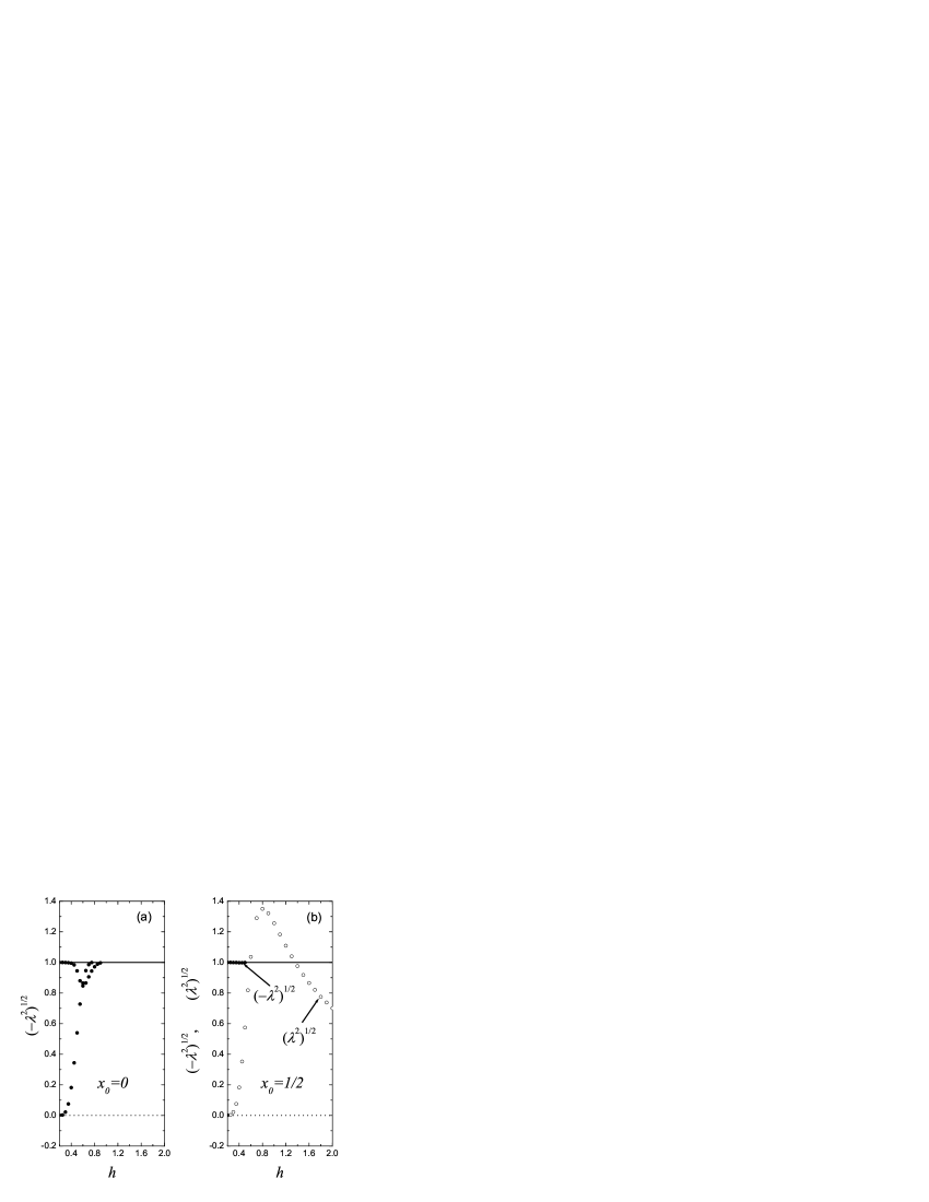
Figure 1: Model $I$, spectrum of the soliton with frequency $\omega=1$ (bottom edge of the continuous spectrum) for (a) stable on-site and (b) unstable inter-site configurations. Spectrum always contains a pair of zero-frequency modes shown by dashed lines. For $h<0.4$ discreteness is weak and the soliton in (a) has a mode with nearly zero frequency corresponding to the translational mode of the continuum NLS equation. The frequency of this mode grows rapidly with increase in $h$ for $h>0.4$ and it enters the continuous band at $h=0.75$ where soliton loses its mobility.

Figure 2: Model $II$, spectrum of the soliton with frequency $\omega=1$ for (a) on-site and (b) asymmetric configurations. Both configurations are stable. A soliton internal mode bifurcates from the bottom edge of the continuous frequency band at rather large $h$. In addition to an always existing pair of zero-frequency modes (shown by dashed lines), for any $x_{0}$, there exist another pair of zero-frequency modes (shown by dots), reflecting the translational invariance of the soliton and the absence of the Peierls-Nabarro potential.

Figure 3: Model $III$, bottom part of the spectrum of the soliton with frequency $\omega=1$ for (a) on-site and (b) inter-site configurations. Both configurations are stable. Soliton internal mode bifurcates from the bottom edge of the continuous frequency band. For any $x_{0}$, the spectrum contains two pairs of zero-frequency modes, which is a common feature for the PNp-free models.

Figure 4: Same as in Fig. 3 but for the top part of the spectrum. In contrast to models $I$ and $II$, the soliton in the model $III$ has internal modes with frequencies lying above the continuous band. Solid line shows the upper edge of the continuous band.

IV.4 Mobility of solitons

Figure 5: Model $I$, $h=0.4$. Time evolution of (a) soliton velocity, (b) norm, (c) modified norm, and (d) momentum. Soliton frequency is $\omega=1$.

Figure 6: Model $I$, $h=0.4$. Time evolution of soliton velocity for different initial velocities. Soliton frequency is $\omega=1$.

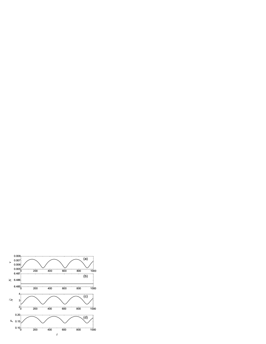
Figure 7: Model $II$, $h=2.0$. Time evolution of (a) soliton velocity, (b) norm, (c) modified norm, and (d) momentum. Soliton frequency is $\omega=1$.

Figure 8: Same as in Fig. 7 but for model $III$.

Solving the eigenvalue problem formulated in Sec. IV.3, we find solutions of corresponding DNLS equation of the form of Eq. (48). Solutions are accurate for small amplitudes of the eigenvectors, $\epsilon_{n}(t)$. Here we examine the solutions corresponding to the translational eigenmode (since “kicks” along this eigendirection may be responsible for/related to motion in these lattices).

We define the position of discrete soliton as its center of mass:

$$S(t)=\frac{\sum nN_{n}(t)}{\sum N_{n}(t)},$$ (52)

where $N_{n}=|\psi_{n}|^{2}$; then the soliton velocity is $v=dS/dt$. This definition is used for $N$-conserving models $I$ and $II$, and for $\tilde{N}$-conserving model $III$, in Eq. (52), we naturally use $\tilde{N}_{n}=(1/4)(\psi_{n}\psi_{-}^{\star}+\psi_{n}^{\star}\psi_{-}+\psi_{n}\psi_{+}^{\star}+\psi_{n}^{\star}\psi_{+})$ instead of $N_{n}$.

Setting initial conditions according to Eq. (48) with sufficiently small amplitude of translational eigenmode $\epsilon_{n}(t)$, we then integrate numerically the DNLS equations to study the soliton mobility at different $h$.

For all three models we boost the solitons initially placed at $x_{0}=0$.

As Fig. 1(a) suggests, the soliton of model $I$ has a translational mode with nearly zero frequency only for $h<0.4$. For such a small $h$, discreteness is weak and model $I$ can be regarded as weakly perturbed continuum NLS equation, which supports moving solitons. However, the frequency of the translational mode increases rapidly for $h>0.4$ and it enters the continuum frequency band at $h=0.75$ when the soliton completely loses its mobility.

In Fig. 5 we show the time evolution of soliton’s velocity, $v$, norm, $N$, modified norm, $\tilde{N}$, and momentum, $P$, for the soliton of frequency $\omega=1$ in model $I$ at $h=0.4$. Soliton was boosted with the initial velocity of $v=0.024$. One can see that norm is conserved while all the other parameters oscillate while the soliton propagates along the chain. The soliton’s velocity is maximum (minimum) when it passes the on-site (inter-site) configuration with minimum (maximum) energy. Its average speed is equal to $0.016$.

To boost the soliton in model $I$ one has to apply sufficiently large initial momentum (i.e., larger than a threshold in order) to overcome the Peierls-Nabarro potential. This feature is illustrated by Fig. 6, where we boost the soliton with different initial velocities: (a) $v_{0}=0.012$, (b) $v_{0}=0.018$, and (c) $v_{0}=0.024$ (same as in Fig. 5). The soliton does not propagate in (a) and in (b), instead, it oscillates near the minimum energy configuration.

The soliton kinematics/dynamics in the PNp-free models $II$ and $III$ are qualitatively different from those in model $I$ because soliton is not trapped by the lattice and thus can be accelerated by even weak external fields.

In Fig. 7 and Fig. 8 we show the results for models $II$ and $III$, respectively, similar to that presented in Fig. 5 for model $I$. Note that for model $I$ we used a rather small discreteness parameter $h=0.4$ while solitons in Fig. 7 and Fig. 8 propagate along highly-discrete chains at $h=2$. It can be clearly seen that model $II$ conserves classical norm $N$, while model $III$ conserves modified norm $\tilde{N}$ and momentum $P$.

V Conclusions

We have described a general and systematic method of constructing spatial discretizations of NLS-type models, whose stationary soliton solutions can be obtained from a two-point difference problem. In this setting, finding stationary solutions becomes tantamount to solving simple nonlinear algebraic equations. We have also illustrated the connections of the resulting models with the integrable discretization of the NLS equation, of which they are a natural generalization for cubic nonlinearities (our construction was given for arbitrary polynomial nonlinearities of a particular parity); furthermore, the differences of such models from the standard discretization of the NLS equation often encountered in physical applications have been highlighted, both in terms of the relevant dynamical (solitonic) behavior as well as in terms of the underlying conservation laws present in the various models.

For the case of cubic nonlinearity we demonstrate that in the constructed PNp-free DNLS chains solitons are stable in a wide range of the discreteness parameter $h$. Semi-analytical moving soliton solutions are found in the regime of propagation at slow speed. Several numerical examples illustrate the qualitative difference in slow soliton dynamics in the classical DNLS equation and the PNp-free DNLS equations. In the classical model to boost the soliton one has to apply sufficiently large initial momentum to overcome the Peierls-Nabarro potential. In the PNp-free model, the soliton behaves differently and can be accelerated by even weak external fields.

We believe that our results may suggest novel possibilities for engineering nonlinear lattices optimized for efficient control over the localization and propagation of discrete solitons in various physical contexts.

References

- (1) J. D. Joannopoulos, R. D. Meade, and J. N. Winn, Photonic Crystals: Molding the Flow of Light (Princeton University Press, Princeton, 1995).
- (2) B. Eiermann, P. Treutlein, T. Anker, M. Albiez, M. Taglieber, K. P. Marzlin, and M. K. Oberthaler, “Dispersion management for atomic matter waves,” Phys. Rev. Lett. 91, 060402–4 (2003).
- (3) D. N. Christodoulides, F. Lederer, and Y. Silberberg, “Discretizing light behaviour in linear and nonlinear waveguide lattices,” Nature 424, 817–823 (2003).
- (4) Yu. S. Kivshar and G. P. Agrawal, Optical Solitons: From Fibers to Photonic Crystals (Academic Press, San Diego, 2003).
- (5) A. Trombettoni and A. Smerzi, “Discrete solitons and breathers with dilute Bose-Einstein condensates,” Phys. Rev. Lett. 86, 2353–2356 (2001).
- (6) B. Eiermann, T. Anker, M. Albiez, M. Taglieber, P. Treutlein, K. P. Marzlin, and M. K. Oberthaler, “Bright Bose-Einstein gap solitons of atoms with repulsive interaction,” Phys. Rev. Lett. 92, 230401–4 (2004).
- (7) D. N. Christodoulides and R. I. Joseph, “Discrete self-focusing in nonlinear arrays of coupled wave-guides,” Opt. Lett. 13, 794–796 (1988).
- (8) Yu. S. Kivshar and D. K. Campbell, “Peierls-Nabarro potential barrier for highly localized nonlinear modes,” Phys. Rev. E 48, 3077–3081 (1993).
- (9) A. B. Aceves, C. De Angelis, T. Peschel, R. Muschall, F. Lederer, S. Trillo, and S. Wabnitz, “Discrete self-trapping, soliton interactions, and beam steering in nonlinear waveguide arrays,” Phys. Rev. E 53, 1172–1189 (1996).
- (10) O. Bang and P. D. Miller, “Exploiting discreteness for switching in waveguide arrays,” Opt. Lett. 21, 1105–1107 (1996).
- (11) W. Krolikowski and Yu. S. Kivshar, “Soliton-based optical switching in waveguide arrays,” J. Opt. Soc. Am. B 13, 876–887 (1996).
- (12) I.E. Papacharalampous, P.G. Kevrekidis, B.A. Malomed and D.J. Frantzeskakis, ”Soliton collisions in the discrete nonlinear Schrödinger equation, Phys. Rev. E 68, 046604-9 (2003).
- (13) R. Morandotti, U. Peschel, J. S. Aitchison, H. S. Eisenberg, and Y. Silberberg, “Dynamics of discrete solitons in optical waveguide arrays,” Phys. Rev. Lett. 83, 2726–2729 (1999).
- (14) A. Fratalocchi, G. Assanto, K. A. Brzdakiewicz, and M. A. Karpierz, “Discrete light propagation and self-trapping in liquid crystals,” Opt. Express 13, 1808–1815 (2005).
- (15) M. J. Ablowitz and J. F. Ladik, “Nonlinear differential-difference equations,” J. Math. Phys. 16, 598–603 (1975).
- (16) M. J. Ablowitz and J. F. Ladik, “Nonlinear differential-difference equations and Fourier- analysis,” J. Math. Phys. 17, 1011–1018 (1976).
- (17) M. Oster, M. Johansson, and A. Eriksson, “Enhanced mobility of strongly localized modes in waveguide arrays by inversion of stability,” Phys. Rev. E 67, 56606–8 (2003).
- (18) Z. Y. Xu, Y. V. Kartashov, and L. Torner, “Soliton mobility in nonlocal optical lattices,” Phys. Rev. Lett. 95, 113901–4 (2005).
- (19) L. Hadzievski, A. Maluckov, M. Stepic, and D. Kip, “Power controlled soliton stability and steering in lattices with saturable nonlinearity,” Phys. Rev. Lett. 93, 033901–4 (2004).
- (20) J. M. Speight and R. S. Ward, “Kink dynamics in a novel discrete sine-Gordon system,” Nonlinearity 7, 475–484 (1994).
- (21) J. M. Speight, “Topological discrete kinks,” Nonlinearity 12, 1373–1387 (1999).
- (22) P. G. Kevrekidis, “On a class of discretizations of Hamiltonian nonlinear partial differential equations,” Physica D 183, 68–86 (2003).
- (23) S. V. Dmitriev, P. G. Kevrekidis, and N. Yoshikawa, “Discrete Klein-Gordon models with static kinks free of the Peierls-Nabarro potential,” J. Phys. A 38, 7617–7627 (2005).
- (24) S. V. Dmitriev, P. G. Kevrekidis, and N. Yoshikawa, “Standard Nearest Neighbor Discretizations of Klein-Gordon Models Cannot Preserve Both Energy and Linear Momentum,” arXiv nlin.PS/0506002 (2005).
- (25) I. V. Barashenkov, O. F. Oxtoby, and D. E. Pelinovsky, “Translationally invariant discrete kinks from one-dimensional maps,” Phys. Rev. E 72, 035602–4 (2005).
- (26) O. F. Oxtoby, D. E. Pelinovsky, and I. V. Barashenkov, “Travelling kinks in discrete phi(4) models,” Nonlinearity 19, 217–235 (2006).
- (27) J. M. Speight and Y. Zolotaryuk, “Kinks in dipole chains,” arXiv nlin.PS/0509047 (2005).
- (28) P. G. Kevrekidis, S. V. Dmitriev, and A. A. Sukhorukov, “On a Class of Spatial Discretizations of Equations of the Nonlinear Schrödinger Type”, submitted for publication (2005); another very recent approach to this problem has just appeared in D. Pelinovsky, “Translationally invariant nonlinear Schrodinger lattices”, nlin.PS/0603022.
- (29) A. Khare, K.Ø. Rasmussen, M.R. Samuelsen and A. Saxena, “Exact Solutions of the Saturable Discrete Nonlinear Schrödinger Equation”, J. Phys. A 38, 807 (2005).
- (30) F. Cooper, A. Khare, B. Mihaila and A. Saxena, “Exact solitary wave solutions for a discrete field theory in 1+1 dimensions”, Phys.Rev. E 72, 036605 (2005).
- (31) A. Khare, K.Ö. Rasmussen, M. Salerno, M.R. Samuelsen and A. Saxena, Discrete Nonlinear Schrödinger Equations with arbitrarily high order nonlinearities nlin.PS/0603034.
- (32) S. V. Dmitriev, P. G. Kevrekidis, N. Yoshikawa, and D. J. Frantzeskakis, “Exact static solutions for some discrete cubic nonlinearity models free of the Peierls-Nabarro potential”, submitted for publication (2006).
- (33) M. Salerno, “Quantum deformations of the discrete nonlinear Schrödinger-equation,” Phys. Rev. A 46, 6856–6859 (1992).
- (34) P. G. Kevrekidis, K. O. Rasmussen, and A. R. Bishop, “The discrete nonlinear Schrödinger equation: A survey of recent results,” Int. J. Mod. Phys. B 15, 2833–2900 (2001).
- (35) J. Carr and J. C. Eilbeck, “Stability of stationary solutions of the discrete self-trapping equation,” Phys. Lett. A 109, 201–204 (1985).