Periodic orbits in scattering from elastic voids

Abstract

The scattering determinant for the scattering of waves from several obstacles is considered in the case of elastic solids with voids. The multi-scattering determinant displays contributions from periodic ray-splitting orbits. A discussion of the weights of such orbits is presented.

1 Introduction

Eventhough the word scattering appears to imply transport, studies of Helmholtz scatterers have shown effects of trapped periodic orbits Predrag . As there is nothing particular about the Helmholtz equation, similar effects are expected for wave equations for other media such as dielectric or elastodynamic ones.

We shall discuss the relation between periodic trapped rays and the scattering determinant corresponding to a medium with several polarizations, each with their own velocity. The example to be treated is the case of elastic wave propagation in a solid punctured by a finite number of voids. These systems have the feature that a ray hitting a boundary can either reflect or refract. Particularly, ray splitting occurs when the polarization changes. This leads to a ray dynamics which no longer is unique, since – in general – a single polarized ray evolves into a tree of rays. A similar behaviour is observed in microwave resonators with dielectrica: characteristically rays can either be reflected or be transmitted at the boundaries of the dielectrica.

2 Scalar case

The Helmholtz equation

$$(\Delta+k^{2})\psi=0$$ (1)

describes the wave propagation of a scalar field $\psi$ of wave number $k$ in a homogeneous and isotropic medium. Furthermore, if obstacles are embedded in this background, the scalar field typically has to satisfy Dirichlet ($\psi=0$) or Neumann ($\partial\psi/\partial n=0$) boundary conditions on the surfaces of the obstacles. For an exterior problem, i.e. a scattering problem, the geometry of the scatterers and the corresponding boundary conditions are usually specified and the typical goal is to calculate the scattering matrix ${\sf S}$. In short, this matrix contains the information on how an incoming wave transforms to a superposition of outgoing scattering solutions. From the knowledge of the scattering matrix several interesting quantities can be calculated: cross-sections, resonances, phase shifts, time-delays etc.

One way of finding the scattering matrix is via the so-called null-field method lloyd ; lloyd_smith ; berry81 ; gaspard ; AW_report ; PetersonStrom ; bostrom ; hwg97 ; cavityThesis . A given field on the boundary of one scatterer gives rise to secondary fields on the full set of boundaries, including the one at infinity. These fields are calculated via boundary integral identities. If a basis is chosen for each boundary, the initial and the secondary fields can be expanded in these bases. The matrices that describe their relationships can be used to construct the scattering matrix gaspard . In this way the application of the standard null-field method determines the ${\sf S}$ matrix as

$${\sf S}={\sf{1}}-i\,{\sf C}\,{\sf M}^{-1}{\sf D},$$ (2)

where the ${\sf C}$ and ${\sf D}$ matrices connect the incoming, respectively, outgoing waves to the interior scattering boundaries and where the matrix ${\sf M}$ relates the waves at one interior scattering boundary to the waves at a different one. ${\sf M}$ itself can be written in terms of a transfer matrix ${\sf A}$ as

$${\sf M}={\sf{1}}+{\sf A}.$$ (3)

The multi-scattering expansion arises when

$${\sf M}^{-1}={\sf{1}}-{\sf A}+{\sf A}^{2}+\dots$$ (4)

is inserted in (2) lloyd ; lloyd_smith ; berry81 ; gaspard . This signals that ${\sf M}$ has the role of an inverse multi-scattering matrix. In some situations the exact matrix elements of these infinite dimensional matrices, ${\sf A}$, ${\sf C}$, and ${\sf D}$, can be derived. Of course these matrices depend crucially on the scattering problem in question, but the overall structure is the same. In general, the null–field method can be applied to solve numerous multi-scattering problems in various media.

An explicit example is the scattering of a scalar wave, propagating in the two-dimensional plane, off a finite number of non-overlapping hard discs that have fixed positions and Dirichlet boundary conditions. For the discussion here only the matrix ${\sf M}$ is of interest. The fields at two different discs $j$ and $j^{\prime}$, expanded in basis states $\exp(im\phi_{j})$ and $\exp(im^{\prime}\phi_{j^{\prime}})$ (in polar coordinates with $m,m^{\prime}=0,\pm 1,\pm 2,\cdots$ two-dimensional angular momentum quantum numbers) are connected via the (transfer) kernel gaspard ; AW_report ; aw_chaos ; aw_nucl ; wh98 ; threeInARow

$$[{\sf A}]_{mm^{\prime}}^{jj^{\prime}}=(1-\delta_{jj^{\prime}})\frac{J_{m}(ka_{j})}{H_{m^{\prime}}^{(1)}(ka_{j^{\prime}})}\,H_{m-m^{\prime}}^{(1)}(kR_{jj^{\prime}})\,e^{im\alpha_{j^{\prime}}^{(j)}-im^{\prime}(\alpha_{j}^{(j^{\prime})}-\pi)}\,.$$ (5)

Here $R_{jj^{\prime}}$ is the center-to-center distance of the discs of radii $a_{j}$, and $\alpha_{j^{\prime}}^{(j)}$ is the angle to the center of cavity $j^{\prime}$ in the coordinate system of cavity $j$. All this follows from the application of the above-sketched null–field method to the scalar-wave problem. Less familiar is the ray limit of the pertinent multi-scattering determinant $\mbox{\rm Det}\,{\sf M}(k)$ gaspard ; AW_report . As the various building blocks of the scattering matrix are known in analytical form it is possible to explicitly calculate the short-wave-length limit. The main result is that asymptotically AW_report

$$\mbox{\rm Det}\,{\sf M}(k)\approx F=\left.\exp\left(-\sum_{p}\sum_{r=1}^{\infty}\frac{1}{r}\,\frac{e^{ir\,(kL_{p}-\nu_{p}\pi/2)}}{|\mbox{\rm Det}\,({\sf{1}}-\mathbf{J}_{p}^{r})|^{1/2}}\,z^{rn_{p}}\right)\right|_{z=1},$$ (6)

where $p$ is a prime orbit (a periodic orbit that cannot be split into shorter ones), $r$ is the number of its repeats, $L_{p}$ is its length, $\nu_{p}$ is its Maslov index, $\mathbf{J}_{p}$ is its monodromy matrix, and $n_{p}$ is its number of bounces on the scatterers. The right-hand side of (6) is the semiclassical spectral determinant Predrag ; gutbook . The parameter $z$, which at the end is put equal to unity, serves in the formal expansion of $F$ in $z$ up to a sufficiently high number $N_{max}\geq n_{p}$. A periodic orbit is defined here as a closed ray in phase space obeying the law of reflection at the scatterers. Our goal is to generalize these types of problems to two-dimensional elastodynamics.

3 Elastodynamics

In isotropic elasticity the wave equation in the frequency domain $\omega$ is

$$\mu\Delta\,{\bf u}+(\lambda+\mu){\bf\nabla(\nabla\cdot u)}+\rho\omega^{2}{\bf u}=0\,,$$ (7)

where ${\bf u}({\bf x})$ is the displacement vector field in the body, $\lambda$, $\mu$ are the material-dependent Lamé coefficients and $\rho$ is the density lAndl ; auld . This wave equation admits two different polarizations: longitudinal L and transverse T with velocities

$$c_{L}=\sqrt{\frac{\lambda+2\mu}{\rho}}\qquad\mathrm{and}\qquad c_{T}=\sqrt{\frac{\mu}{\rho}}\,.$$ (8)

The longitudinal and transverse waves correspond to pressure, respectively, shear deformations (or to primary and secondary arriving pulses in seismology). This leads to the law of refraction for incoming plane waves

$$\frac{c_{L}}{c_{T}}=\frac{\sin\theta_{L}}{\sin\theta_{T}},$$ (9)

where $\theta_{L}$, $\theta_{T}$ denote the angle of incidence or reflection of the longitudinal and transverse wave, respectively, measured with respect to the normal to the surface.

The stress tensor in elasticity has the form

$$\sigma_{ij}=\lambda\,\partial_{k}u_{k}\delta_{ij}+\mu\left(\partial_{i}u_{j}+\partial_{j}u_{i}\right)\,.$$ (10)

The boundary conditions considered here are free. Hence

$${\bf t}({\bf u})\equiv\mbox{\boldmath{$\sigma$}}({\bf u})\cdot{\bf n}=\biggl{[}\lambda\Bigl{(}{\bf\nabla}\cdot\bf{u}\Bigr{)}{\bf 1}+\mu\Bigl{\{}\bigl{(}{\bf\nabla}\bf{u}\bigr{)}+\bigl{(}{\bf\nabla}\bf{u}\bigr{)}^{\mathsf{T}}\Bigr{\}}\biggr{]}\cdot{\bf{n}}={\bf 0}$$ (11)

for the displacement field at the boundary where $\mathbf{n}$ denotes the normal to the boundary and $\mathsf{T}$ indicates a transposition. The operator $\mathbf{t}$ refers to the traction.

4 Scattering determinant

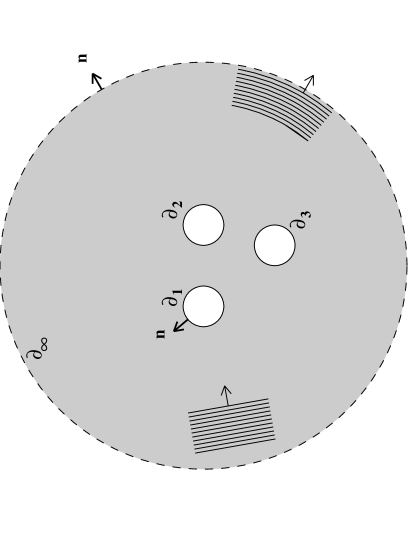
Figure 1: General zone of two–dimensional cavity scattering. Here the unit vectors ${\bf n}$ denote the outside normals to the surfaces $\partial_{i}$ ($i=1,2,3$) of the cavities or to the surface $\partial_{\infty}$ of the total scattering zone. Furthermore, an incoming plane wave and a scattered cylindrical wave are shown.

As mentioned, in this treatment the medium corresponds to a cylindrical solid made, for simplicity, of an isotropic and homogeneous elastic material. The scattering geometry consists of parallel cylindrical voids, which are perpendicular to the endcaps of the overall cylinder, see fig. 1. If the fields are stimulated by in-phase line-sources parallel to the voids, this symmetry is respected and the problem reduces to one of two-dimensional elasticity, see Fig. 1, referred to as plane strain. This scattering problem generalizes the simpler scalar scattering off discs in two dimensions, mentioned in sect. 2.

Similar to the scalar case AW_report ; wh98 ; hwg97 , the scattering determinant may be factorized into an incoherent single-scatterer part (in terms of the determinants over the single-scattering matrices ${\sf S}^{(1)j}(\omega)$, $j=1,2,\cdots$) and the genuine multi-scatterer part (in terms of the determinant of the inverse multi-scattering matrix ${\sf M}(\omega)$) cavityThesis

$${\mbox{\rm det}\,}{{\sf S}}(\omega)=\left\{\!\prod_{{j}\in\mathrm{Cavities}}\mbox{\rm det}{}{\bigl{[}{\sf S}^{(1)j}(\omega)\bigr{]}}\!\right\}\frac{{\mbox{\rm Det}\,}\bigl{[}{{\sf M}}(\omega^{\ast})^{\dagger}\bigr{]}}{{\mbox{\rm Det}\,}\bigl{[}{{\sf M}}(\omega)\bigr{]}}.$$ (12)

When the relative positions of the cavities are changed, only the latter factor, composed from the cluster determinant $\mbox{\rm Det}\,\,{\sf M}(\omega)$, changes:

$${\sf M}={\bf 1}+{\sf A}\,,$$ (13)

$$\Bigl{[}{{\sf A}}^{jj^{\prime}}_{ll^{\prime}}\Bigr{]}_{ii^{\prime}}=(1\!-\!\delta_{jj^{\prime}})\frac{a_{j}}{a_{j^{\prime}}}\sum_{\sigma=L}^{T}\sum_{\sigma^{\prime}=L}^{T}\bigl{[}{\sf t}_{l}^{(J)j}\bigr{]}_{i\sigma}\Bigl{[}{\sf T}^{(+)jj^{\prime}}_{ll^{\prime}}\Bigr{]}_{\sigma\sigma^{\prime}}\bigl{[}{\sf t}_{l^{\prime}}^{(+)j^{\prime}}\bigr{]}^{-1}_{\sigma^{\prime}i^{\prime}}\,,$$

$$\Bigl{[}{\sf T}^{(+)jj^{\prime}}_{ll^{\prime}}\Bigr{]}_{\sigma\sigma^{\prime}}=\delta_{\sigma\sigma^{\prime}}H_{l-l^{\prime}}^{(+)}(k_{\sigma}R_{jj^{\prime}})e^{il\alpha_{j^{\prime}}^{(j)}-il^{\prime}(\alpha_{j}^{(j^{\prime})}-\pi)}.$$

The indices $i,i^{\prime}\in\{r,\phi\}$ are the labels of the two-dimensional polar coordinates and the indices $\sigma,\sigma^{\prime}\in\{L,T\}$ refer to the two polarization states. The diagonal matrix $\Bigl{[}{\sf T}^{(+)jj^{\prime}}_{ll^{\prime}}\Bigr{]}$ may be interpreted as a translation matrix acting on the polarized scattering states, where $k_{L}=\omega/c_{L}$ and $k_{T}=\omega/c_{T}$ are the pertinent wave numbers PetersonStrom ; bostrom . As in (5), $R_{jj^{\prime}}$ is the center-to-center distance of the circular cavities of radii $a_{j}$ and $\alpha_{j^{\prime}}^{(j)}$ is the angle to the center of cavity $j^{\prime}$ in the coordinate system of cavity $j$. The single-cavity scattering matrices (enumerated by the cavity index $j=1,2,\dots$) are separable in the (two-dimensional) angular momentum $l=0,\pm 1,\pm 2,\cdots$ due to the rotational symmetry. They have the general form:

$$\bigl{[}{\sf S}^{(1)j}_{l}\bigr{]}=-\bigl{[}{\sf t}_{l}^{(+)j}\bigr{]}^{-1}\cdot\bigl{[}{\sf t}_{l}^{(-)j}\bigr{]}$$ (14)

in terms of the $2\times 2$ traction matrices $\bigl{[}{\sf t}_{l}^{(Z)j}\bigr{]}$ which incorporate the free boundary conditions (11). Here the “type” $Z\in\{+,-,J\}$ refers to outgoing, incoming or regular scattering states and involves $H_{l}^{(1)}$, $H_{l}^{(2)}$ or $J_{l}$ Bessel functions of argument $z_{L,T}\equiv ak_{L,T}$, respectively. Thus we have, e.g., for the outgoing case:

$$\small{\bigl{[}{\sf t}_{l}^{(+)j}\bigr{]}}=\frac{2\mu}{a_{j}^{2}}\,\pmatrix{{(l^{2}-z_{T}^{2}/2)H^{(1)}_{l}(z_{L})-z_{L}\frac{dH^{(1)}_{l}(z_{L})}{dz_{L}}}&{i\,l\left(H^{(1)}_{l}(z_{T})-z_{T}\frac{dH^{(1)}_{l}(z_{T})}{dz_{T}}\right)}\cr{i\,l\left(H^{(1)}_{l}(z_{L})-z_{L}\frac{dH^{(1)}_{l}(z_{L})}{dz_{L}}\right)}&{-(l^{2}-z_{T}^{2}/2)H^{(1)}_{l}(z_{T})+z_{T}\frac{dH^{(1)}_{l}(z_{T})}{dz_{T}}}\cr}\,.$$ (15)

Note that the single-cavity scattering matrix connects different polarizations. For a full discussion, see cavityThesis ; izbicki ; paoAndmow ; cavityLetter . The connection to the interior problem of a single disc is described in disc .

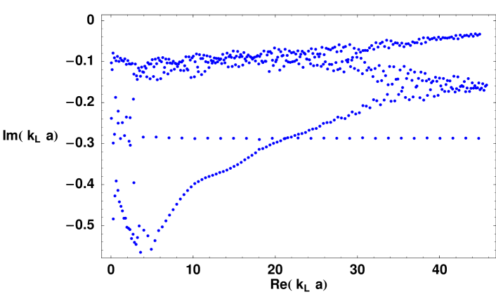
Figure 2: Elastodynamic scattering resonances from cavityLetter for two cavities of common radius $a$ ($A_{1}$-representation, center-to-center-separation $R=6a$) in the complex longitudinal Helmholtz number–plane: $k_{L}a=\omega a/c_{L}$.

As first shown for the scalar problem AW_report , the poles of the cluster determinant $\mbox{\rm Det}\,{\sf M}(\omega)$ cancel – by construction – the poles of the single-scattering determinants. Likewise, the poles of $\mbox{\rm Det}\,{\sf M}(\omega^{*})$ are canceled by the zeros of the single-scattering determinants. Thus all scattering resonances defined by the poles of the scattering determinant ${\mbox{\rm det}\,}{{\sf S}}(\omega)$ can be found from the zeros of the cluster determinant $\mbox{\rm Det}\,{\sf M}(\omega)$ AW_report ; wh98 . As an example consider the resonances in fig. 2, see cavityLetter , of a two–cavity system made of polyethylene izbicki , a material with $c_{L}=1950$ m/s and $c_{T}=540$ m/s. Furthermore, it is assumed that the cavity radii are equal, i.e. $a_{1}=a_{2}\equiv a$, and that the inter-cavity separation $R$, measured from the centers, is 6 times larger than $a$. Note that the regular spaced horizontal set of resonances in fig. 2 is placed below an irregular set. This is opposite to the scalar Helmholtz case for the same geometry where the regular spaced resonances are above the irregular ones vwr94 ; vattay94 ; threeInARow ; rvw96 . The regular resonances particular to the fundamental $A_{1}$-representation are well described by the following condition aw_chaos

$$0=1+\exp(ik_{L}L)/\sqrt{\Lambda}$$ (16)

with the length $L=4a$ and instability $\Lambda=5+2\sqrt{6}$ Predrag . $L$ corresponds to the length of the shortest periodic orbit moving in a symmetry–reduced domain spanned by the surface of the cavity and the center-of-mass of the two cavities. $\Lambda$ is obtained from the product of ray matrices as the leading eigenvalue of the monodromy matrix gutbook ; Predrag of the corresponding (geometric acoustic) ray system. This next raises the question about the effect of the remaining set of orbits.

5 Orbits in time–delay

For real frequencies the total scattering phase $\Theta$ is given by the sum over the cluster phase $\Theta_{c}$ and the single cavity phases $\Theta_{j}$:

$$\Theta(\omega)=\frac{1}{2i}\ln\,\mbox{\rm det}\,S(\omega)\qquad\mathrm{and}\qquad\Theta_{c}(\omega)=\frac{1}{2i}\ln\frac{\mbox{\rm Det}\,\,M(\omega^{\ast})^{\dagger}}{\mbox{\rm Det}\,\,M(\omega)}\,,$$ (17)

see (12). Likewise, the derivative with respect to frequency $d\Theta/d\omega$, the Wigner-Smith time delay, can be decomposed into single-scatterer and cluster contributions. The numerics of the cluster time–delay $d\Theta_{c}/d\omega$ show fluctuations which are related to trapped periodic orbits in the scattering geometry, see fig. 3 where the results for two identical cavities (the same system as in fig. 2) are presented. Due to the symmetry of the system the cluster delay decomposes further into a sum over four irreducible representations of the symmetry group $C_{2v}$ hamermesh , of which the representations $A_{1}$ and $B_{2}$ are shown. Some of these orbits are diffractive (see cavityThesis ; cavityLetter for more details) including segments of surface propagation of Rayleigh type, which are also important in earthquakes viktorov . For these proceedings we focus the discussion to purely non-diffractive contributions, called geometrical ray-splitting orbits.

Figure 3: Power spectrum of the time–delays derived from the cluster phase shift of two cavities of common radius $a$ and center-to-center separation $R=6a$. The thick and thin line denote the $A_{1}$- and $B_{2}$-representation, respectively. The symbols P$i$ and S$i$ label, in turn, periodic orbits with $i$ legs of pressure or shear polarization. The circular arcs indicate Rayleigh–surface waves.

6 Expanding the cluster determinant

As in the scalar case AW_report , a central point in the orbit-construction is the definition of the cluster determinant in terms of traces:

$${F}(z)=\mbox{\rm Det}\,({\sf{1}}+z\,{\sf A})\equiv\exp\left(-\sum_{n=1}^{\infty}\frac{z^{n}\,\mbox{Tr}\,(-{\sf A})^{n}}{n}\right)\,,$$ (18)

where $z$ is again a formal expansion parameter which is put equal to one at the end. Equation (18) holds if ${\sf A}$ is trace–class, and its Taylor expansion is called the cumulant expansion aw_chaos ; aw_nucl ; AW_report ; wh98 . Trace-class operators (or matrices) are those, in general, non-Hermitian operators (matrices) of a separable Hilbert space which have an absolutely convergent trace in every orthonormal basis reed_simon ; simon . Especially the determinant $\mbox{\rm Det}\,({\sf{1}}+z{\sf A})$ exists and is an entire function of $z$, if ${\sf A}$ is trace-class. Presently the trace-class property of ${\sf A}$ has only been proved in detail in the two-dimensional scalar case AW_report ; wh98 and sketched for the three-dimensional case in hwg97 . Nevertheless, we shall proceed as if this is true also in our elastodynamical case. This is supported by the following numerical evidences: (i) the sum over the moduli of the eigenvalues of the matrix ${\sf A}$ from (13) is absolutely converging in agreement with the expected trace-class property of this matrix; (ii) the determinant (18) converges to a finite result as the dimension of ${\sf A}$ is increased beyond a minimal number $N_{\rm dim}>2\times\left(\frac{e}{2}(c_{L}/c_{T})|k_{L}|a\right)$, see cavityLetter and also AW_report ; berry81 ; and (iii) the resonances of the cumulant expansion truncated at fourth order $z^{4}$ agree very well with the exact ones plotted in fig. 2, see cavityLetter .

7 Ray limit and orbits

The expansion (18) indicates that the cluster determinant can be obtained from the knowledge of an increasing number of traces. Moreover, each trace $\mbox{Tr}\,{\sf A}^{n}$ is given by the sum over all exact periodic itineraries of topological length $n$, see AW_report . In the saddle-point approximation the periodic itineraries become the periodic orbits of topological length $n$, which means that they bounce $n$ times between the cavities AW_report . These orbits fulfill the laws of reflection and refraction and have phases corresponding to their time periods of revolution $T_{p}$.

A periodic itinerary of topological length $n$ corresponds to a cyclic product of $n$ terms involving one operator of the type

$$\bigl{[}{\sf t}_{l}^{(+)j}\bigr{]}^{-1}\cdot\bigl{[}{\sf t}_{l}^{(J)j}\bigr{]}$$ (19)

(which corresponds to the ${\sf T}$-matrix-part (times $-1/2$) of a single-cavity scattering matrix (14)) followed by one translation operator $\Bigl{[}{\sf T}^{(+)jj^{\prime}}_{ll^{\prime}}\Bigr{]}$ (the free propagation). The pruning rule that two successive scatterings must take place at different cavities is automatically built in (see the term $(1-\delta_{jj^{\prime}})$ in the kernel ${\sf A}$). The ray limit of the single cavity ${\sf T}$-matrix gives unitary reflection coefficients similar to those of the scattering from an infinite half–plane lAndl ; disc . This leads to an overall amplitude $\alpha_{p}$ defined as a product over all reflection coefficients along the orbit. This amplitude describes the leakage from the orbit due to ray splitting.

The calculation of the geometric amplitudes of the orbits requires more work. See shudo for a general discussion with respect to the interior scalar case and AW_report for the exterior counter part. Asymptotic wave theory indicates kellerPTD ; KellerElasto ; rulf ; achenbach that for open trajectories in two dimensions the amplitude scales as $(kR)^{-1/2}$ where $k$ is the wave number in question and $R$ is the radius of curvature of the wave front at the observer. This radius is studied in e.g. geometric optics. It it is possible to keep track of its evolution in the free-propagation period between the scatterers and at impacts including possible refractions with the help of suitable ray matrices cavityThesis . Indeed, for our problem it can be shown that all those open segments that have fixed end points, but intermediate points (variables) determined by saddle-point integrations, have such an amplitude evolution. This comes about by calculating the accompanying sparse Hessian of this restricted integration.

For a full saddle-point integration over all variables, in other words for a periodic orbit $p$, the amplitude turns out to be expressible as yet another sparse Hessian that can be expanded into Hessians of the type of the previously considered open pieces; see AW_report for the scalar case. The use of the previous information then allows the full calculation with the amplitude evolving as

$$\mathcal{A}_{p}=\frac{\alpha_{p}}{|\mbox{\rm Det}\,({{\sf{1}}-\mathbf{J}_{p}})|^{1/2}}\,\,z^{n_{p}}\,,$$ (20)

where $\mathbf{J}_{p}$ is the product of the ray matrices and and $\alpha_{p}$ is the product of the reflection coefficients, calculated along the orbit $p$ with its $n_{p}$ bounces. This form is precisely part of the conventional semiclassical density of states gutbook ; brack ; Stock . However, the formal parameter $z$ is also present and can be seen as a counting and ordering parameter of the various orbits in the expansion over infinitely many orbits Predrag ; artuso1 ; artuso2 .

Incorporating the results of the geometric ray-splitting orbits gives the following factor of the ray-dynamical approximation of the cluster determinant:

$${F}_{G}(z)=\exp\left(-\sum_{p}\sum_{r=1}^{\infty}\frac{1}{r}\,{\alpha}_{p}^{r}\,\frac{e^{ir\,\omega T_{p}}}{|\mbox{\rm Det}\,({\sf{1}}-\mathbf{J}_{p}^{r})|^{1/2}}\,z^{rn_{p}}\right)\,.$$ (21)

The sum over $r$ counts the repeats of the primary periodic orbits, the prime cycles $p$. If the logarithmic derivative with respect to $\omega$ is taken, a result very similar to the spectral density for the interior problem is obtained. This is in agreement with the general result for the density of states for ray-splitting systems described in couch . Similar results for the case of flexural vibrations in the interior case are given in HB . As the orbits are unstable and $\mathbf{J}_{p}$ is symplectic, it is possible to expand, for each orbit, the instability denominator in (21) in the inverse of its leading eigenvalue $1/\Lambda_{p}$ and to obtain a so-called Gutzwiller–Voros resummed zeta function similar to those of two-dimensional Hamiltonian flows Predrag :

$${F}_{G}(z)=\prod_{k=0}^{\infty}\,\zeta_{k}^{-1}(z)\,,$$ (22)

where

$$1/\zeta_{k}(z)=\prod_{p}(1-t_{p}^{(k)})\quad\mbox{with}\quad t_{p}^{(k)}={\alpha}_{p}\,\frac{e^{i\omega T_{p}}}{\sqrt{|\Lambda_{p}|}\Lambda_{p}^{k}}\,z^{n_{p}}\,.$$ (23)

8 Summary

Detailed studies of Helmholtz scattering determinants at small wave lengths have shown the influence of periodic orbits. The case of scattering from voids in two–dimensional elastodynamics was considered here with a discussion of the analytical contribution of periodic ray-splitting orbits to the scattering determinant.

References

- (1) P. Cvitanović, R. Artuso, R. Mainieri and G. Vattay, Classical and Quantum Chaos, www.nbi.dk/ChaosBook/, Niels Bohr Institute, Copenhagen, 2005.
- (2) P. Lloyd, Proc. Phys. Soc. 90, 207 (1967).
- (3) P. Lloyd and P. V. Smith, Adv. Phys. 21, 69 (1972).
- (4) M. V. Berry, Ann. Phys. (N.Y.) 131, 163 (1981).
- (5) P. Gaspard and S. Rice, J. Chem. Phys. 90, 2225; 2242; 2255 (1989).
- (6) A. Wirzba, Phys. Rep. 309, 1 (1999).
- (7) B. Peterson and S. Ström, J. Acoust. Soc. Am. 56, 771 (1974).
- (8) A. Boström, J. Acoust. Soc. Am. 67, 399 (1980).
- (9) N. Søndergaard, Wave Chaos in Elastodynamic Scattering, www.nbi.dk/nsonderg, thesis, Northwestern University (Evanston, 2000) (unpublished).
- (10) M. Henseler, A. Wirzba, and T. Guhr, Ann. Phys. (N.Y.) 258, 286 (1997).
- (11) A. Wirzba and M. Henseler, J. Phys. A 31, 2155 (1998).
- (12) A. Wirzba, Chaos 2, 77 (1992).
- (13) A. Wirzba, Nucl. Phys. A 560, 136 (1993).
- (14) A. Wirzba and P. E. Rosenqvist, Phys. Rev. A 54, 2745 (1996).
- (15) M. C. Gutzwiller, Chaos in Classical and Quantum Mechanics (Springer, New York, 1990).
- (16) L. D. Landau and E. M. Lifshitz, Theory of Elasticity (Pergamon, Oxford, 1959).
- (17) B. A. Auld, Acoustic Fields and Waves in Solids I,II (John Wiley and Sons, New York, 1973).
- (18) J. L. Izbicki, J. M. Conoir and N. Veksler, Wave Motion 28, 277 (1998).
- (19) Y. H. Pao and C. C. Mow, Diffraction of Elastic Waves and Dynamic Stress Concentrations (Rand Corporation, New York, 1971).
- (20) A. Wirzba, N. Søndergaard, P. Cvitanović, Europhys. Lett. 72, 534 (2005) [nlin.CD/0108053].
- (21) N. Søndergaard and G. Tanner, Phys. Rev. E 66, 066211 (2002).
- (22) G. Vattay, A. Wirzba, and P. E. Rosenqvist, Phys. Rev. Lett. 73, 2304 (1994).
- (23) G. Vattay, A. Wirzba and P. E. Rosenqvist, Proc. Int. Conference on Dynamical Systems and Chaos, edited by Y. Aizawa, S. Saito and K. Shiraiwa (World Scientific, Singapore, 1995), Vol. 2, pp. 463-466, chao-dyn/9408005.
- (24) P. E. Rosenqvist, G. Vattay, and A. Wirzba, J. Stat. Phys. 83, 243 (1996).
- (25) M. Hamermesh, Group Theory and Its Applications to Physical Problems (Addison-Wesley, Reading, 1962).
- (26) I. A. Viktorov, Rayleigh and Lamb waves (Plenum Press, New York, 1967).
- (27) M. Reed and B. Simon, Analysis of Operators, Methods of Modern Mathematical Physics, (Academic, New York, 1978), Vol. IV, Chap. XIII, Sec. 17.
- (28) B. Simon, Adv. Math. 24, 244 (1977).
- (29) T. Harayama and A. Shudo, Phys. Lett. A 165, 417 (1992).
- (30) J. B. Keller and F. C. Karal, Jr., Journ. of Appl. Phys. 31, 1039 (1960).
- (31) J. B. Keller and F. C. Karal, Jr., J. Acoust. Soc. Am. 36, 32 (1964).
- (32) B. Rulf, Journ. of Acoust. Soc. Am. 45, 493 (1969).
- (33) J. D. Achenbach, A. K. Gautesen and H. McMaken, Ray Methods for Waves in Elastic Solids (Pitman, Boston, 1982).
- (34) M. Brack and R. K. Bhaduri, Semiclassical Physics (Addison-Wesley, Reading, 1997).
- (35) H.-J. Stöckmann, Quantum Chaos: An Introduction (Cambridge University Press, 1999).
- (36) R. Artuso, E. Aurell and P. Cvitanović, Nonlinearity 3, 325 (1990).
- (37) R. Artuso, E. Aurell and P. Cvitanović, Nonlinearity 3, 361 (1990).
- (38) L. Couchman, E. Ott and T. M. Antonsen, Jr., Phys. Rev. A 46, 6193 (1992).
- (39) E. Bogomolny and E. Hugues, Phys. Rev. E 57, 5404 (1998).