Turbulent Relative Dispersion in Two-Dimensional Free Convection Turbulence

Abstract

The relative dispersion process in two-dimensional free convection turbulence is investigated by direct numerical simulation. In the inertial range, the growth of relative separation, $r$, is expected as $\langle r^{2}(t)\rangle\propto t^{5}$ according to the Bolgiano–Obukhov scaling. The result supporting the scaling is obtained with exit-time statistics. Detailed investigation of exit-time PDF shows that the PDF is divided into two regions, the Region-I and -II, reflecting two types of separating processes: persistent expansion and random transitions between expansion and compression of relative separation. This is consistent with the physical picture of the self-similar telegraph model. In addition, a method for estimating the parameters of the model are presented. Comparing two turbulence cases, two-dimensional free convection and inverse cascade turbulence, the relation between the drift term of the model and nature of coherent structures is discussed.

I Introduction

Relative dispersion of passive particles in turbulent flows is one of the fundamental problems in turbulence research. It characterizes the transport and mixing properties of turbulence and is important from both theoretical and practical points of view. Reflecting universal behavior of turbulent fluctuations, relative dispersion also has some universal properties because of its locality-in-scale nature Batchelor (1950); Monin and Yaglom (1975); Fung and Vassilicos (1998). In particular, the dispersion process exhibits anomalous dispersion in the inertial range. This is first observed by Richardson (1926) Richardson (1926), and since then, a number of theoretical, experimental, and numerical investigations have been devoted to understand and model relative dispersion process Jullien et al. (1999); Ott and Mann (2000); Ishihara and Kaneda (2002); Boffetta and Sokolov (2002a, b); Goto and Vassilicos (2004); Rivera and Ecke (2005); Sawford (2001). However, comprehensive understanding has not been obtained yet.

Recently, a few works focusing on underlying mechanism of the anomalous dispersion were reported. In the inertial range, the mean free path, $l(r)$, the mean length for persistent expansion of relative separation without changing its moving direction, is an order of relative separation itself, $r$: $l(r)=P_{s}r$ Sokolov (1999); Sokolov et al. (2000). Here, $P_{s}$ is a non-dimensional constant called the persistent parameter. In two-dimensional inverse cascade turbulence (2D-IC), $P_{s}$ is estimated as $0.87$ Boffetta and Sokolov (2002a). This means separating motions are not purely diffusive but composed of an appreciable amount of persistent motions. In addition, it was also reported that there is a relation between stagnation-point structures and Richardson’s law Dávila and Vassilicos (2003), and that dispersion process is described by persistent streamline topology Goto and Vassilicos (2004). From these results, it is expected that coherence of turbulent field, which must share its origin with fine coherent vortical structures such as worms in three-dimensional Navier-Stokes (3D-NS) turbulence, has a significant role in turbulent relative dispersion.

The correlations in turbulence are characterized in scale-space due to their self-similarity, and are not made disappear by coarse graining in real space. Reflecting these correlations, relative separation moves persistently to some extent, so that, unlike the Brownian motion, relative separation process should not be described only by random collision motions even as an approximationSokolov (1999). In other words, the characteristic length cannot be defined because the mean free path, $l(r)$, varies depending on the spatial scale. Whereas there are several experiments and numerical simulations of which results are rather close to the prediction of Richardson’s diffusion equation Jullien et al. (1999); Boffetta and Sokolov (2002a); Goto and Vassilicos (2004) that closely relates to random collision motions. Thus, these results raise a question; how are the effects of persistent motions wiped out? In the previous paper Ogasawara and Toh (2005a), we have introduced a self-similar telegraph model of turbulent relative dispersion, and showed that the separation PDF can be close to the prediction of Richardson’s diffusion equation for slowly separating particle pairs even in the presence of persistent motions.

In the present paper, we check the consistency of the physical picture of the self-similar telegraph model by carrying out direct numerical simulations (DNS) of 2D free convection (2D-FC) turbulence instead of 3D-NS turbulence. This is because (i) DNS of 3D-NS turbulence requires extremely large computer resources, so that it is difficult to track particles for a long time, which is necessary to investigate dynamical properties of relative dispersion process, and (ii) 2D-FC turbulence has both statistical and dynamical characteristics similar to those of 3D-NS turbulence (see Appendix A) Toh and Suzuki (1994); Toh and Matsumoto (2003). Among them, the existence of coherent structures, which are approximated by the Burgers T-Vortex layer, is notable. This is a crucial difference from coherent structures in 2D-IC turbulence that are nested cat’s eye vortices Fung and Vassilicos (1998); Goto and Vassilicos (2004). Therefore, comparing the results of the 2D-FC case with those of the 2D-IC case, we can investigate the effects of coherent structure on turbulent relative dispersion. This comparison gives a physical meaning of the drift term of the self-similar telegraph model.

The inertial range achieved by our DNS is not so wide that the relative motions of particle-pairs in the dissipation, the inertial, and the energy containing scales are not sufficiently resolved by usual fixed time statistics. In order to investigate the scaling natures of relative dispersion in such a narrow and limited inertial range, we utilize exit-time statistics introduced into research of turbulent relative dispersion by Boffetta and Sokolov (see Appendix B) Artale et al. (1997); Boffetta et al. (1999); Boffetta and Sokolov (2002a). By detailed investigation of the PDF of exit-time, we show that the PDF is divided into two region, the Region-I and -II, corresponding to persistent expansion and random transition between expansion and compression of relative separation, respectively. This result agrees with the picture of the self-similar telegraph model. In addition, we provide a method for estimation of the parameters of the self-similar telegraph model by using exit-time PDF.

In the following sections, first we provide a brief review of the self-similar telegraph model in §2. Section 3 presents a summary of the numerical scheme and parameters of our DNS of 2D-FC turbulence. Some of the results by the fixed-time and the exit-time statistics are provided and discussed in §4. Concluding remarks are made in §5. In addition, some properties of 2D-FC turbulence and exit-time statistics are presented in Appendix A and B, respectively.

II Self-similar telegraph model and Palm’s equation

In the previous paper Ogasawara and Toh (2005a), we have introduced a self-similar telegraph model for turbulent relative dispersion, which is a model describing the evolution of the PDF of relative separation of particle pairs in the inertial range. The relative separation of two particles, $r(t)$ is defined as follows:

$$r(t)=|\bm{x}_{1}(t)-\bm{x}_{2}(t)|,$$ (1)

where $\bm{x}_{1}(t)$ and $\bm{x}_{2}(t)$ are the Lagrangian positions of the particles. The model is based on Sokolov’s model Sokolov (1999) and consists of persistent expansion and compression of relative separation, $r$, according to the relative velocity, $v(r)=\check{A}r^{1-s}$, where $\check{A}$ and $s$ are a dimensional constant and a scaling exponent, respectively: $s=2/3$ for Kolmogorov scaling and $s=2/5$ for Bolgiano-Obukhov scaling. The transition rate from expansion to compression and that from compression to expansion are given by $\lambda^{+}/T_{c}(r)$ and $\lambda^{-}/T_{c}(r)$, respectively. Here $T_{c}(r)$ is a characteristic time scale at a spatial scale $r$, $T_{c}(r)=\check{A}^{-1}r^{s}$, and $\lambda^{\pm}$ are the inverses of persistent parameters, $P_{+}$ for expansion and $P_{-}$ for compression. Introducing $\lambda=\lambda^{+}+\lambda^{-}$ and $\delta=\lambda^{+}-\lambda^{-}$, the evolution equation of the separation PDF, $P(r,t)$, is derived as follows:

$$\frac{T_{c}(r)}{\lambda}\frac{\partial^{2}P}{\partial t^{2}}+\frac{\partial P}{\partial t}=\frac{\partial}{\partial r}\left[D(r)r^{d-1}\frac{\partial}{\partial r}\left(\frac{P}{r^{d-1}}\right)\right]$$

$$+\sigma\frac{\partial}{\partial r}\left[v(r)P\right],$$ (2)

where $D(r)$ is Richardson’s diffusion coefficient, $\check{A}\lambda^{-1}r^{2-s}$, and $\sigma=(d-2s+\delta)\lambda^{-1}\equiv\tilde{\sigma}\lambda^{-1}$. The parameters of the model are $\lambda$ and $\delta$: $\lambda$ represents the strength of persistency of moving directions, and $\delta$ does the difference in persistency between expansion and compression. Therefore, $\lambda$ and $\delta$ reflect the strength and structure of coherence of the flow, respectively.

For slowly-separating particle pairs, i.e., in the case of $r\ll\langle r^{2}\rangle^{1/2}$, the first term of the l.h.s. of Eq. (2) can be neglected and the approximated equation is given by

$$\frac{\partial P}{\partial t}=\frac{\partial}{\partial r}\left[D(r)r^{d-1}\frac{\partial}{\partial r}\left(\frac{P}{r^{d-1}}\right)\right]+\sigma\frac{\partial}{\partial r}\left[v(r)P\right].$$ (3)

This form of the equation was first derived by Palm Monin and Yaglom (1975) and is also the same as the diffusion equation of Goto-Vassilicos model Goto and Vassilicos (2004). We call Eq. (3) Palm’s equation. The similarity solution of Eq. (3) is

$$P(r,t)=C_{P}t^{-\frac{1}{s}}\left(\frac{\lambda r^{s}}{s^{2}\check{A}t}\right)^{\frac{d-\tilde{\sigma}-1}{s}}\exp\left(-\frac{1}{s^{2}}\frac{\lambda r^{s}}{\check{A}t}\right),$$ (4)

where $C_{P}$ is the normalization factor.

Because the tail of the exit-time PDF, $P_{E}(T_{E};r,\rho)$, consists of slowly-separating particle pairs, it is calculated from Palm’s equation (3) with the method used by Boffetta and Sokolov Boffetta and Sokolov (2002a). The asymptotic form of $P_{E}(T_{E};r,\rho)$ is given by

$$P_{E}(T_{E};r,\rho)\qquad\qquad\qquad\qquad\qquad\qquad\qquad\quad$$

$$\sim\exp\left(-\frac{1}{4}\frac{sj^{2}_{1-\frac{\delta}{s},1}}{2s-\delta}(1-\rho^{-s})\frac{T_{E}}{\langle T_{E}(r;\rho)\rangle}\right),$$ (5)

where $j_{\nu,n}$ is the $n$-th zero of the $\nu$-th order Bessel function and $\langle T_{E}(r;\rho)\rangle$ is the mean exit-time from $r$ to $\rho r$:

$$\langle T_{E}(r;\rho)\rangle=\frac{\lambda}{\check{A}}\frac{1}{s(2s-\delta)}\left(\rho^{s}-1\right)r^{s}.$$ (6)

Note that the mean exit-time calculated from the self-similar telegraph model, Eq. (2), is the same as Eq. (6). This is because the mean exit-time is calculated from a steady solution of the equation Boffetta and Sokolov (2002a), and the solution of Eq. (2) is the same as that of Eq. (3). By comparing the tail of the exit-time PDF obtained by DNS and Eq. (5), we can estimate the value of $\delta$.

The last term of the r.h.s. of Eq. (2) is a drift term consistent with the scaling law, and the direction of the drift is determined by $\tilde{\sigma}$. The parameter $\tilde{\sigma}$ consists of two parts, the “scaling-determined” one, $d-2s$, and the “dynamics-determined” one, $\delta$. In order for Eq. (3) to recover Richardson’s equation, the drift term has to disappear, which means $\delta=2s-d\equiv\delta_{0}$. We call this case the Richardson case or the zero-drift case, where the parameters of the model reduce to one, $\lambda^{+}$; $\lambda^{-}$ is determined by the relation $\lambda^{-}=\lambda^{+}-\delta_{0}\equiv\lambda^{-}_{0}$.

III Numerical Simulation

Figure 1: Rescaled energy and entropy spectrum $\tilde{E}(k)$ and $\tilde{S}(k)$ obtained by DNS at resolution $N=1024$ (NV10) and $N=2048$ (NV11). The straight lines refer to the Bolgiano-Obukhov scaling: $\tilde{E}(k\eta_{\theta})\equiv\eta_{\theta}^{-3}\tau_{\theta}^{-2}E(k)$, $\tilde{S}(k\eta_{\theta})\equiv\eta_{\theta}^{-1}\epsilon_{\theta}^{-1}\tau_{\theta}^{-1}S(k)$.

Table 1: Parameters used in the present DNS.

label	$N$	$\nu$	$f_{0}$	$d_{0}$	$k_{d}$
NV10	$1024$	$1\times 10^{-4}$	$5\times 10^{-2}$	$1\times 10^{-1}$	3
NV11	$2048$	$5\times 10^{-5}$	$5\times 10^{-2}$	$1.5\times 10^{-1}$	10

Table 2: Characteristic quantities of generated turbulent fields. $\Delta x$ represents the grid size.

label	$\epsilon_{\theta}$	$\eta_{\theta}$	$\tau_{\theta}$	$\lambda_{x}$	$\lambda_{y}$	$\text{Ra}_{\lambda}$
NV10	$7.11\times 10^{-3}$	$5.87\times 10^{-3}$ ($0.956\Delta x$)	$3.44\times 10^{-1}$	$4.50\times 10^{-2}$	$4.54\times 10^{-2}$	$2.50\times 10^{3}$
NV11	$1.44\times 10^{-2}$	$3.49\times 10^{-3}$ ($1.14\Delta x$)	$2.43\times 10^{-1}$	$3.01\times 10^{-2}$	$3.03\times 10^{-2}$	$3.99\times 10^{3}$

In this section, we explain the method of DNS used in the present work and show basic properties of turbulent fields produced by our simulation.

We generate turbulent field by DNS of the vorticity equation with a large-scale friction term $F_{d}$ and the temperature equation with a large-scale forcing term $F_{f}$:

$$\nabla\cdot\bm{u}=0,$$ (7)

$$\frac{\partial\omega}{\partial t}+(\bm{u}\cdot\nabla)\omega=\nu\triangle\omega+\alpha g\frac{\partial T}{\partial x}+F_{d},$$ (8)

$$\frac{\partial T}{\partial t}+(\bm{u}\cdot\nabla)T=\kappa\triangle T+F_{f},$$ (9)

where $\omega$, $T$, $\bm{u}$, $\nu$, $\kappa$, $\alpha$, and $g$ represent the vorticity field, the temperature field, the velocity field, the kinematic viscosity, the thermal diffusivity, the thermal expansion coefficient, and the gravitational acceleration, respectively. The large-scale forcing term used here is

$$F_{f}(\bm{x})=4f_{0}\cos(2x)\cos(2y),$$ (10)

where $f_{0}$ is a constant. The large-scale friction term is written in the Fourier space as

$$\hat{F}_{d}(\bm{k})=\begin{cases}-\frac{d_{0}}{|\bm{k}|^{2}}\hat{\omega}(\bm{k})&(0<|\bm{k}|\leq k_{d}),\\ 0&(\text{otherwise}),\end{cases}$$ (11)

where $d_{0}$, $\bm{k}$, $\hat{F}_{d}(\bm{k})$, and $\hat{\omega}(\bm{k})$ are a constant, the wave number vector, the Fourier mode of the friction term, and the Fourier mode of the vorticity field, respectively. Our DNS is performed on a $2\pi\times 2\pi$ domain with the doubly periodic boundary conditions at resolutions $N^{2}$: $N=1024$ (NV10) and $2048$ (NV11). We employ a pseudo-spectral method for accurately calculating convolutions and spatial derivatives, and 4-th order Runge-Kutta method for time integration. Aliasing error is removed by adopting the phase-shift method (NV10) and the $3/2$ method (NV11). All results presented in this paper are obtained for statistically stationary and locally isotropic turbulence. We summarize the parameters used in our simulation in Table 1 and characteristic quantities of generated turbulence in Table 2.

Figure 1 shows the entropy and energy spectra obtained by our DNS. The spectra are rescaled with entropy dissipation scales and the entropy dissipation rate, and there is a region consistent with the Bolgiano-Obukhov scaling, Eqs. (29) and (30), (see Appendix A). We call this region the inertial range. Most investigations in the present paper are carried out in this range.

In the velocity field generated by DNS, we track a number of particle pairs ($1\times 10^{6}$ pairs) according to the advection equation:

$$\frac{\partial}{\partial t}\bm{x}_{i}(t)=\bm{u}(\bm{x}_{i}(t),t),$$ (12)

where $\bm{x}_{i}(t)$ is the position of the $i$-th particle at time $t$. We employ the 4-th order Runge-Kutta method for numerical integration, and the linear interpolation to obtain the velocity of each particles. Particle pairs are distributed homogeneously with relative separation of the grid scale $\Delta x$ at the initial time.

IV Results and discussion

IV.1 Fixed-time statistics

Figure 2: Temporal evolution of mean relative separation $\langle r(t)^{p}\rangle$ obtained in the case of NV11. Solid, dotted and dashed line refer to $p=1/2,1,$ and $2$, respectively. Straight lines indicate Richardson’s law. The inset shows the local slope of $\langle r(t)^{p}\rangle$.

Figure 3: The PDF of relative separation $r$ obtained in the case of NV11. Different marks refer to different time: open box, closed box, open circle, and closed circle refer to $t=1.2$, $1.6$, $2.0$, and $2.4$, respectively. (a) the non-rescaled plot, (b) the rescaled plot with $\langle r^{2}\rangle^{1/2}$. The solid, dashed, and dotted lines are the similarity solutions of Palm’s equation Eq. (3) with $\delta=-0.77$, $-1.2$, and $-0.06$, respectively. The inset shows the linear plot of a blowup of the head region.

First, we briefly discuss the results obtained by standard fixed-time statistics, which concerns the distribution of relative separation at a certain (fixed) time.

In Fig. 2 we plot temporal evolutions of the mean relative separation of particle pairs, $\langle r^{p}\rangle$, for different powers, $p=1/2$, $1$, and $2$. In the cases of $p=1/2$ and $1$, the generalized Richardson’s relations, $\langle r^{p}\rangle\propto t^{5p/2}$, are realized, though the times at which they start and the time intervals in which they hold differ. These differences result from the limited width of the inertial range in DNS. For example, in the case of NV11, the inertial range is roughly estimated as $80<r/\Delta x<320$. From Fig. 3(a), it is clear that the separation PDF broadens rapidly, so that $\langle r^{p}\rangle$ is contributed to by a quite broad range of relative separation including the dissipation, the inertial, and the energy containing ranges. As a result, the weight of each range varies with the power of the moment of the relative separation and thus, the range of time in which the contribution of the inertial range dominates differs accordingly. The slope of $\langle r^{2}\rangle$ is less steep than Richardson’s law. This is because, in the case of $p=2$, the contribution of particle pairs in the energy containing range to $\langle r^{p}\rangle$ is much larger than that in the cases of $p=1$ and $1/2$. In the energy containing range, relative separation process is described by the Brownian motion, $\langle r^{2}\rangle\propto t$, which is less steep than Richardson’s law. Hence, the larger the contribution of the range is, the less steep the slope of $\langle r^{p}\rangle$ is.

Even though the Richardson’s law is observed for $p=1/2$ and $1$, the fact doesn’t necessarily support the validity of the Richardson’s law because it is reported that the temporal evolution of $\langle r^{p}\rangle$ strongly depends on the initial separation of particle pairs Boffetta and Sokolov (2002a); Goto and Vassilicos (2004). Hence we have to check the scaling law by adopting a different method that is independent of the initial separation.

In order to check self-similarity of the PDF of relative separation, we plot the PDF rescaled with $\langle r^{2}\rangle^{1/2}$ in Fig. 3(b). The values of $\langle r^{2}\rangle^{1/2}$ at $t=1.2$, $1.6$, $2,0$, and $2.4$ are $15.3$, $28.6$, $47.5$, and $72.0\Delta x$, respectively. All PDFs collapse well for $r/\langle r^{2}\rangle^{1/2}<10$ and they are in good agreement with the similarity solution of Palm’s equation with $\delta=-0.06$. However, we cannot conclude that the temporal evolution of the separation PDF is self-similar and governed by Palm’s equation because Fig. 3(b) is obtained not from separations only in the inertial range but in the much wider range, $0<r<720\Delta x$. Although the collapse in Fig. 3(b) implies existence of a self-similar stage governed by Palm’s equation, we have not had any reasonable explanation of the collapse.

IV.2 Exit-time statistics

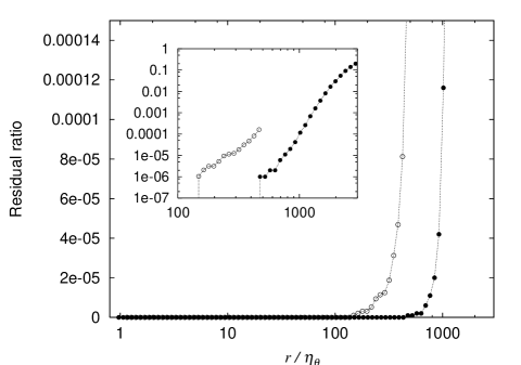
Figure 4: Residual ratio of particle pairs. Dotted lines with open and closed circles refer to data obtained by DNS at resolution $N=1024$ (NV10) and $N=2048$ (NV11) respectively. The inset is the log-log plot of the ratio.

Figure 5: Scale dependence of the mean exit-time $\langle T_{E}(\delta;\rho)\rangle$ for $\rho=1.1$ rescaled with the dissipation time scale, $\tau_{\theta}$. Open and closed circles refer to the results obtained by the present DNS at resolution $N=1024$ (NV10) and $N=2048$ (NV11), respectively. The inset is the compensated plot with $(\rho^{s}-1)(r/\eta_{\theta})^{2/5}$. The dashed line represents estimated values of the coefficients $C_{E}^{\mathrm{(BO)}}\approx 2.6$.

Figure 6: Mean exit-time and the residual ratio for several time steps ($\rho=1.1$): open box, closed box, open triangle, and closed circle represent $t=20$, $30$, $40$, and $60$, respectively. (a) the residual ratio for several time step, (b) the scale dependence of the mean exit-time.

Figure 7: The PDF of exit-time for $\rho=1.1$ in the case of NV11. (a) the non-rescaled PDF, (b) the rescaled PDF with the mean exit-time $\langle T_{E}(r;\rho)\rangle$. The solid, dashed, dotted and dashed-dotted lines refer to $r=80,129,208$ and, $335\Delta x$, respectively. The insets show a semi-log plot of the PDF.

IV.2.1 Mean exit-time

The scale dependence of the mean exit-time obtained by our DNS is shown in Fig. 5. It is observed that, although the width is narrow, there is a region consistent with the Bolgiano-Obukhov scaling, $\langle T_{E}(r;\rho)\rangle\propto r^{2/5}$. The exit-time statistics is independent of initial separation of particle pairs if spatial scale $r$ is large enough for them to forget information of their initial conditions Boffetta and Sokolov (2002a); Goto and Vassilicos (2004). In our simulation, the initial separation of particle pairs is $\Delta x$ that is much smaller than the scales in which the scaling law holds. Therefore, this result indicates that Richardson’s law is valid in the 2D-FC turbulence.

According to the scaling law, the form of the mean exit-time is given by

$$\frac{\langle T_{E}(r;\rho)\rangle}{\tau_{\theta}}=C_{E}^{\mathrm{(BO)}}(\rho^{s}-1)\left(\frac{r}{\eta_{\theta}}\right)^{s},$$ (13)

where $C_{E}^{\mathrm{(BO)}}$ is considered to be a universal constant. The inset of Fig. 5 shows a compensated plot of the mean exit-time. Although the weak $\mathrm{Ra}_{\lambda}$ dependence of $C_{E}^{\mathrm{(BO)}}$ seen in Fig. 5 requires higher resolution of DNS to more accurate estimation, $C_{E}^{\mathrm{(BO)}}$ is estimated as $2.6$ in the present DNS.

In order to obtain statistically reliable data of exit-time, it is important that the residual ratio of particle pairs must be small enough to take in slowly separating particle pairs. The residual ratio at a scale $r$ and a time $t$ is defined as the ratio of particle pairs of which first passage times at $r$ are less than $t$. If the residual ratio is not small enough at the time when statistics of exit-time are calculated, the statistics cannot reflect slowly separating particle pairs. Figure 4 shows the residual ratio of particle pairs used in the present work at the termination time of DNS, $t=60$. It is obvious that the ratio is almost zero in the inertial range, so that our exit-time data is reliable in the sense mentioned above. Figure 6(b) shows the scale dependence of the mean exit-time obtained from insufficient data and illustrates the importance of the residual ratio. Although the results at $t=20$ seem to have the wider inertial range than others, it is a fake. Therefore, to obtain statistically reliable data, we have to track particle pairs until the residual ratio becomes at least less than $0.1\%$.

In contrast to the inertial range, the mean exit-time is almost constant in the dissipation range ($r/\eta_{\vartheta}\lesssim 30$ in Fig. 5) except in the initial transient region, because the relative velocity is proportional to relative separation: $v(r)\propto r$. The exit-time, then, is given by

$$\int_{r}^{\rho r}\frac{dr^{\prime}}{v(r^{\prime})}\propto\int_{r}^{\rho r}\frac{dr^{\prime}}{r^{\prime}}=\log\rho=\mathrm{Const.}$$ (14)

Note that the mean exit-times rescaled by $\tau_{\theta}$ collapse each other in Fig. 5. This is because there is only one characteristic time scale, $\tau_{\theta}$, in the dissipation range Batchelor (1952).

IV.2.2 PDF of exit-time and distribution of particle pairs in real space

We plot exit-time PDF, $P_{E}(T_{E};r,\rho)$, in the inertial range in Fig. 7(a), and that rescaled by the mean exit-time, $\langle T_{E}(r;\rho)\rangle$, in Fig. 7(b). Obviously the PDFs of different scales collapse onto one curve in Fig 7(b). This means exit-time PDF is self-similar in the inertial range and indicates that relative dispersion process is self-similar.

As is clear from Fig. 7(b), the exit-time PDF consists of two regions: the sharp peak and the long exponential tail. We call these two regions the Region-I and the Region-II, respectively. The qualitative difference in form between these indicates that the PDF reflects two different types of motions. In order to clarify the difference, snapshots of typical distribution of particle pairs in the Region-I and -II are shown in Figs. 8 and 9, respectively, with a snapshot of the magnitude of T-Vorticity field $|\bm{\chi}|$.

 

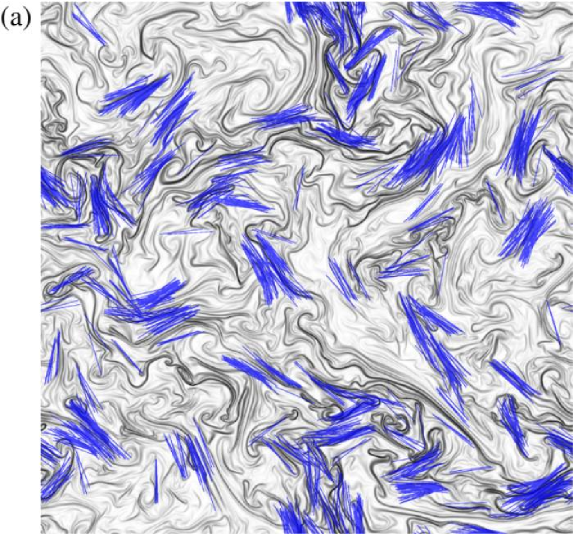
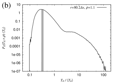
Figure 8: Distribution of particle pairs in the Region-I, $0.3<T_{E}/\langle T_{E}\rangle<0.35$, for $r=80.2\Delta x$ and $\rho=1.1$ at $t=8$ in the case of NV10. (a) the distribution of particle pairs superimposed onto a snapshot of the modulus of T-Vorticity, $|\bm{\chi}|$. Shading represents intensity of $|\bm{\chi}|$. A particle pair is represented by a line segment (particles are located at both ends of the line segment). The whole computational domain is shown. (b) the PDF of exit-time rescaled with the mean. The particle pairs drawn in (a) belong to the gray region, $0.3<T_{E}/\langle T_{E}\rangle<0.35$.

 

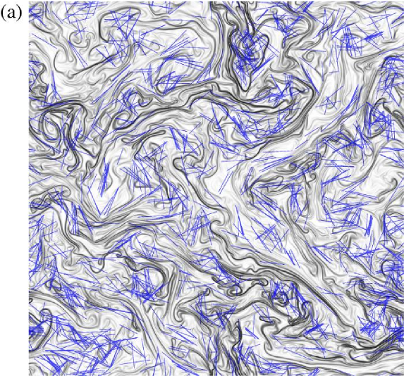
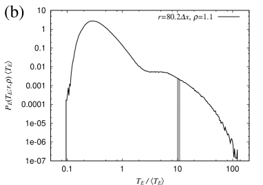
Figure 9: Distribution of particle pairs in the Region-II, $10<T_{E}/\langle T_{E}\rangle<11$, for $r=80.2\Delta x$ and $\rho=1.1$ at $t=8$ in the case of NV10. (a) and (b) are drawn in the same manner as Fig. 8.

Figure 10: Temporal evolution of relative separation for several particles in the case of NV11. Different lines represent different particle pairs.

In Fig. 8(a), on the snapshot of $|\bm{\chi}|$ at $t=8$ ($\equiv t_{s}$), we plot line segments representing particle pairs of which exit-time $T_{E}(r_{s};\rho_{s})$ for $r_{s}=80.2\Delta x$ and $\rho_{s}=1.1$ satisfies $0.3<T_{E}/\langle T_{E}(r_{s};\rho_{s})\rangle<0.35$, that is, $T_{E}(r_{s};\rho_{s})$ is in the shaded region in Fig. 8(b). In order to select such particle pairs, we first extract pairs satisfying the condition $0.3<T_{E}/\langle T_{E}(r_{s};\rho)\rangle<0.35$, and then pick out ones of which first passage times at $r_{s}$ are smaller than $t_{s}$ and those at $\rho r_{s}$ are larger than $t_{s}$. Figure 9(a) is drawn by the same procedure. To draw Figs. 8 and 9, we used the data of NV10.

In 2D-FC turbulence, fine coherent structures are well approximated by the Burgers T-Vortex layer, so that shear layers are formed around the structures Toh and Matsumoto (2003). In addition, such structures are persistent in time to some extent. Hence, particles around the coherent structures are advected along them and relative separations of the particles expand or compress persistently. We call this type of motion the persistent separation. As is shown in Fig. 8(a), particle pairs in the Region-I appear to be along the fine coherent structures. Moreover relative separations of particle pairs in Fig. 8(a) expand rapidly as can be known by their short exit-time. Therefore, Fig. 8 supports the picture of persistent separations.

In contrast to the Region-I, the distribution of particle pairs in the Region-II is in disorder (see Fig. 9(a)). Because the particle pairs contained in the Region-II have long exit-time, the longitudinal relative velocity of them remains small positive during the passage from $r_{s}$ to $\rho r_{s}$ or moving direction of relative separation of the pairs changes from expansion to compression at least once before they reach $\rho r_{s}$. However it is quite unlikely that relative velocity remains small positive for a long time, so that the latter is probably the main mechanism of the formation of the Region-II. Hence, it is expected that both of expanding and compressing pairs are contained in Fig. 9(a). In fact, there are several pairs placed along coherent structures, which probably are expanding. Note that their relative separations are not confined to be larger than $r_{s}$. In addition, there are also pairs across the structures, which are presumably compressing because the structures are approximated by the Burgers T-Vortex layer. Moreover, some pairs are located at positions where the fine coherent structures twist. The twisted regions are generated when well-stretched structures lose their activities and are folded, or when the structures are generated by plumes. Therefore the particle pairs in such regions are changing their moving directions from expansion to compression or the opposite.

Figure 10 shows five typical evolutions of particle-pair separation. Sample 3 expands persistently without any strong compression but Sample 4 experiences both persistent expansion and compression several times. The former corresponds to motions along structures and belongs to the Region-I; the latter does across structures or twisted region and belongs to the Region-II. Note that even a single evolution contains motions that are categorized into the Region-I or into the Region-II. These facts are consistent with the assumptions of the self-similar telegraph model: relative separation process consists of persistent expansion and compression with some random transition mechanisms.

IV.2.3 Estimation of $\delta$

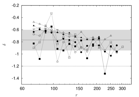
Figure 11: Estimated values of $\delta$ in the case of NV11. Dotted lines with open box, closed box, open circle, closed circle, open triangle, closed triangle, and reverse open triangle denote $\rho=1.1^{1/8}$, $1.1^{1/4}$, $1.1^{1/2}$, $1.1$, $1.1^{2}$, $1.1^{4}$, and $1.1^{8}$, respectively. Solid and dashed lines indicate the mean value, $\delta=-0.77$, and the value of the Richardson’s case, $\delta=-1.2$, respectively. The shaded region represents the standard deviation.

It is expected that expansion and compression of relative separation differ in persistency; the former is experienced mainly by particle pairs along coherent structures and the latter does by those across the structures. Since the auto-correlations of strain and temperature along the structures have longer characteristic lengths than those across them in 2D-FC turbulence Toh and Matsumoto (2003), expanding motions must be more persistent than compressing ones. So as to confirm this consideration, we investigate the slope of the tail of the exit-time PDF. Then, with Eq. (5), we estimate $\delta$ that describes the difference in persistency between expansion and compression of relative separation.

Note that using the asymptotic form of the exit-time PDF calculated from Palm’s equation, Eq. (5), may be justified as follows. Introducing a time scale $\bar{t}$, the l.h.s. of the self-similar telegraph model, Eq. (2), is rewritten as follows:

$$\mathrm{l.h.s.}=\frac{T_{c}(r)}{\lambda\bar{t}}\frac{1}{\bar{t}}\frac{\partial^{2}P}{\partial\hat{t}^{2}}+\frac{1}{\bar{t}}\frac{\partial P}{\partial\hat{t}},$$ (15)

where $\hat{t}=t/\bar{t}$. In the case that $\bar{t}\gg T_{c}(r)/\lambda$ at a certain spatial scale $r$, the first term of the l.h.s. can be neglected, and thus, the model is reduced to Palm’s equation. Hence, the tail of the exit-time PDF by the telegraph model, which consists of slowly-separating particle pairs, must coincide with that by Palm’s equation. It is also easy to show that the mean exit-time is the same between Eqs. (2) and (3). We, therefore, adopt Eq. (5) for the estimation of $\delta$.

Figure 11 shows the estimated values of $\delta$ in the inertial range. The mean value of $\delta$ is $-0.77$ and the standard deviation is $\pm 0.17$. This negative value denotes that expanding motions are more persistent than compressing ones, which supports the above expectation.

In addition, $\delta$ is larger than that of the Richardson case (the zero-drift), $\delta=-1.2\equiv\delta_{0}$. Because $\delta=\lambda^{+}-\lambda^{-}$, $\delta>\delta_{0}$ means $\lambda^{-}<\lambda^{+}-\delta_{0}\equiv\lambda^{-}_{0}$, that is, the compressing motion of relative separation is more persistent than that of the Richardson case. This fact results in the negative drift in the self-similar telegraph model, Eq. (2). The negativity of the drift can be accepted considering that coherent structures in 2D-FC turbulence are string-like and scale-transversal ones Toh and Matsumoto (2003). That is, because the coherent structures in 2D-FC turbulence are not nested in scales, there are few obstacles to compressing motions. On the other hand, the typical structures in 2D-IC turbulence are nested vortices called “cat’s eye in a cat’s eye”. A separation process of particle pairs in 2D-IC turbulence, thus, is a step-by-step one each step of which consists of a trapping by one of nested vortices and sudden separation into a next larger vortex Goto and Vassilicos (2004); compressing motions are probably blocked by the nested vortices. In fact, the estimated values of $\delta$ from DNS of 2D-IC turbulence by Boffetta & Sokolov Boffetta and Sokolov (2002a) and Goto & Vassilicos Goto and Vassilicos (2004) are smaller than that of the Richardson case Ogasawara and Toh (2005a); the compressing motion of relative separation is less persistent than the Richardson case. This results in the positive drift in Eq. (2). We, therefore, conclude that the drift term in the self-similar telegraph model, Eq. (2), reflects the characteristics of coherent structures of the flow.

IV.2.4 Comparison of the Region-II with a solution of Palm’s equation

Figure 12: Rescaled PDF of exit-time ($r=107\Delta x$) in the case of NV11 and the prediction of Palm’s equation ($\delta=-0.77$) for several values of $\rho$. Solid and dashed lines refer to the results of DNS and that obtained from Palm’s equation through the relation Eq. (46).

In Fig. 12, we compare the PDF of exit-time obtained by DNS with that calculated from Palm’s equation by Eq. (46). In the Region-I, the form of the PDF by DNS is totally different from that by Palm’s equation. In the Region-II, however, the two PDFs collapse onto a single curve even when $\rho$ is very small, and thus, the separation process of particle pairs in the Region-II can be described by Palm’s equation, Eq. (3). This indicates that the motion of particle pair is diffusive in the Region-II; the separating process from $r\rho^{-1}$ to $r$ doesn’t affect that from $r$ to $r\rho$. It is also observed that the form of the exit-time PDF varies depending on the value of $\rho$ in Fig. 12. The larger the value of $\rho$ is, the larger the proportion of the Region-II becomes. If $\rho$ is sufficiently large, the whole PDF seems to be occupied by the Region-II and the relative separation process is substantially described by Palm’s equation, Eq. (3).

As mentioned in the previous subsection, the tail of the exit-time PDF calculated from the self-similar telegraph model, $P_{E}^{\mathrm{(T)}}(T_{E};r,\rho)$, must agree with that calculated from Palm’s equation, $P_{E}^{\mathrm{(P)}}(T_{E};r,\rho)$. In addition, as the value of $\rho$ gets larger, the region of $P_{E}^{\mathrm{(T)}}(T_{E};r,\rho)$ overlapping with $P_{E}^{\mathrm{(P)}}(T_{E};r,\rho)$ expands. This is because, for large values of $\rho$, most of exit-times of particle pairs are longer than the characteristic time $T_{c}(r)/\lambda$. Hence, the self-similar telegraph model probably has the same properties as the results shown in Fig. 12.

IV.2.5 Characteristics of the Region-I and estimation of $\lambda$

Figure 13: Rescaled PDF of exit-time ($r=107\Delta x$) in the case of NV11. The peak value is normalized to be unity. Different lines represent different values of $\rho$: $\rho=4.59$, $2.14$, $1.46$, $1.21$, $1.1$, $1.05$, $1.02$, and $1.01$ from the curve with the lowest cut-off rescaled exit-time to that with the highest. The inset is the same plot in linear scale.

Figure 13 shows the exit-time PDF for NV11 rescaled with $\langle T_{E}(r;\rho)\rangle$ and normalized by their peak values. It is clear that the shape of the Region-I is independent of $\rho$. That is, there exists a $\rho$-independent function representing the shape of the exit-time PDF in the Region-I, $\widehat{P}_{E}^{\mathrm{(I)}}(\widetilde{T}_{E})$. Here, $\widetilde{\ \ }$ denotes rescaling by the mean exit-time, $\langle T_{E}(r;\rho)\rangle$. We assume that $\widehat{P}_{E}$ is normalized as $\int_{0}^{\infty}\widehat{P}_{E}(\widetilde{T}_{E})d\widetilde{T}_{E}=1$. Then, in the Region-I, the exit-time PDF is written as

$$\widetilde{P}_{E}(\widetilde{T}_{E};\rho)=W(\rho)\widehat{P}_{E}^{\mathrm{(I)}}(\widetilde{T}_{E}),$$ (16)

where $W(\rho)$ is a normalization factor depending on $\rho$. The exit-time PDF, $\widetilde{P}_{E}(\widetilde{T}_{E};\rho)$, takes the peak value at $\widetilde{T}_{E}^{\mathrm{max}}$. It is estimated that $\widetilde{T}_{E}^{\mathrm{max}}\approx 0.3$ in Fig. 13, which can be regarded as a characteristic time scale of the Region-I. As shown in the inset of Fig. 13, $\widehat{P}_{E}^{\mathrm{(I)}}(\widetilde{T}_{E})$ distributes sharply around $\widetilde{T}_{E}^{\mathrm{max}}$.

If the Region-I is formed by particle pairs of which relative separations expand persistently according to $v(r)=\check{A}r^{1-s}$, the exit-time in the Region-I, $T_{E}^{\mathrm{(I)}}(r;\rho)$, is given by the pass through time from $r$ to $\rho r$:

$$T_{E}^{\mathrm{(I)}}(r;\rho)=\int_{r}^{\rho r}\frac{dr}{v(r)}=\frac{(\rho^{s}-1)r^{s}}{s\check{A}}.$$ (17)

Then, using the general form of the mean exit-time, Eq. (44), the exit-time rescaled by $\langle T_{E}(r;\rho)\rangle$ in the Region-I, $\widetilde{T}_{E}^{\mathrm{(I)}}(r;\rho)$, is

$$\widetilde{T}_{E}^{\mathrm{(I)}}(r;\rho)\equiv\frac{T_{E}^{\mathrm{(I)}}(r;\rho)}{\langle T_{E}(r;\rho)\rangle}=\frac{1}{s\check{C}_{E}\check{A}},$$ (18)

which is independent of $\rho$. Thus, $\widehat{P}_{E}^{\mathrm{(I)}}(\widetilde{T}_{E})$ can be connected to the PDF of $\check{A}$, $P_{\check{A}}(\check{A})$, which is the PDF of Lagrangian relative velocity, $v(r)$, rescaled with $r^{1-s}$:

$$\widehat{P}_{E}^{\mathrm{(I)}}(\widetilde{T}_{E})=\widehat{P}^{\mathrm{(I)}}_{E}\left(\frac{1}{s\check{C}_{E}\check{A}}\right)\equiv s\check{C}_{E}\check{A}^{2}P_{\check{A}}(\check{A}).$$ (19)

Note that $P_{\check{A}}(\check{A})$ is expected to be independent both of $r$ and $\rho$. Since, in the self-similar telegraph model, the distribution of the coefficient, $\check{A}$, of the relative velocity is not considered, $P_{\check{A}}(\check{A})$ is a $\delta$-function: $P_{\check{A}}(\check{A})=\delta(\check{A}-\check{A}_{c})$. Accordingly, the Region-I of the exit-time PDF is approximated by a $\delta$-function at $\widetilde{T}_{E}^{\mathrm{(I)}}$ in the model.

Combining Eqs. (6) and (18), we can estimate $\lambda$ from $\widetilde{T}_{E}^{\mathrm{(I)}}$. From Eq. (6), $\check{C}_{E}$ in the case of the self-similar telegraph model is given by

$$\check{C}_{E}=\frac{\lambda}{\check{A}}\frac{1}{s(2s-\delta)}.$$ (20)

Then, $\lambda$ is calculated as follows:

$$\lambda=\frac{2s-\delta}{\widetilde{T}_{E}^{\mathrm{(I)}}}.$$ (21)

If we assume that $\widetilde{T}_{E}^{\mathrm{(I)}}\approx\widetilde{T}_{E}^{\mathrm{max}}\approx 0.3$, then, $\lambda$ is estimated as $5.2$. However, the value of $\widetilde{T}_{E}^{\mathrm{(I)}}$ is not necessarily well defined. Roughly speaking, it may take a value satisfying $0.19\lesssim\widetilde{T}_{E}^{\mathrm{(I)}}\lesssim 0.45$, if assuming $\widetilde{T}_{E}^{\mathrm{(I)}}$ is in the half-value width of the Region-I around $\widetilde{T}_{E}^{\mathrm{max}}$. Then, the estimated value of $\lambda$ is in the range, $3.5\lesssim\lambda\lesssim 8.3$.

V concluding remarks

We have investigated relative dispersion in 2D free convection turbulence by direct numerical simulation. In the inertial range, where the entropy cascade dominates, we have confirmed with exit-time statistics that relative dispersion satisfies the Bolgiano-Obukhov scaling and, therefore, is self-similar. It was also shown that the exit-time PDF, $P_{E}(T_{E};r,\rho)$, is divided into two parts, the Region-I and -II, and that both of them satisfy the scaling-law and the self-similarity. $P_{E}(T_{E};r,\rho)$ is written as the following form:

$$P_{E}(T_{E};r,\rho) \!\!\!= \!\!\!H(T_{E}^{\mathrm{div}}(r;\rho)-T_{E})P_{E}^{\mathrm{(I)}}(T_{E};r,\rho)\qquad\quad$$ (22)

$$\!\!\!+ \!\!\!H(T_{E}-T_{E}^{\mathrm{div}}(r;\rho))P_{E}^{\mathrm{(II)}}(T_{E};r,\rho),$$

where $T_{E}^{\mathrm{div}}(r;\rho)$ is a division time-scale (exit-time) between the Region-I and -II, and $H(x)$ is a smoothed step function such that $H(x)=0$ if $x\ll 0$ and $H(x)=1$ if $x\gg 0$. $P_{E}^{\mathrm{(I)}}(T_{E};r,\rho)$ and $P_{E}^{\mathrm{(II)}}(T_{E};r,\rho)$ correspond to the exit-time PDF of the Region-I and -II, respectively. The investigation of the distribution of particle pairs in the real space indicates that the Region-I and -II are formed, respectively, by particle pairs expanding along coherent structures and by those experiencing turns between expansion and compression (Figs. 8 and 9).

Figures 13 and 12 show the following characteristics of $P_{E}^{\mathrm{(I)}}(T_{E};r,\rho)$ and $P_{E}^{\mathrm{(II)}}(T_{E};r,\rho)$. The form of $P_{E}^{\mathrm{(I)}}(T_{E};r,\rho)$ is independent of $\rho$ if it is rescaled with the mean exit-time. Moreover, if we assume that the Region-I is constituted by persistently-separating particle pairs, the form of $P_{E}^{\mathrm{(I)}}(T_{E};r,\rho)$ is related to the PDF of Lagrangian relative velocity, $v(r)=\check{A}r^{1-s}$. That is,

$$\widetilde{P}_{E}^{\mathrm{(I)}}(\widetilde{T}_{E};\rho)=\frac{W(\rho)}{s\check{C}_{E}\widetilde{T}_{E}^{2}}P_{\check{A}}\left(\frac{1}{s\check{C}_{E}\widetilde{T}_{E}}\right),$$ (23)

where $W(\rho)$ is a $\rho$-dependent normalization factor, and $P_{\check{A}}(\check{A})$ is the PDF of $v(r)$ rescaled with $r^{1-s}$. On the other hand, $P_{E}^{\mathrm{(II)}}(T_{E};r,\rho)$ agrees with the exit-time PDF calculated from Palm’s equation, $P_{E}^{\mathrm{(P)}}(T_{E};r,\rho)$, the form of which varies depending on $\rho$ even when it is rescaled with $\langle T_{E}(r;\rho)\rangle$. Hence $\widetilde{P}_{E}(\widetilde{T}_{E};\rho)$ is written as

$$\widetilde{P}_{E}(\widetilde{T}_{E};\rho) \!\!\!= \!\!\!\widetilde{H}(\widetilde{T}_{E}^{\mathrm{div}}(\rho)-\widetilde{T}_{E})\frac{W(\rho)}{s\check{C}_{E}\widetilde{T}_{E}^{2}}P_{\check{A}}\left(\frac{1}{s\check{C}_{E}\widetilde{T}_{E}}\right)$$ (24)

$$\!\!\!+ \!\!\!\widetilde{H}(\widetilde{T}_{E}-\widetilde{T}_{E}^{\mathrm{div}}(\rho))\widetilde{P}_{E}^{\mathrm{(P)}}(\widetilde{T}_{E};\rho).$$

Figure 14: Similarity solution (fixed-time PDF of relative separation) of the self-similar telegraph model in the case of 2D-FC turbulence. The parameters used in this figure are estimated from DNS data for NV11 by using the exit-time PDF. Different lines refer to different values of $\lambda$. $\lambda=\infty$ corresponds to the similarity solution of Palm’s equation. The inset is a blowup of the head region in the linear scale.

These results support the self-similar telegraph model. In the model, $\widetilde{P}_{E}^{\mathrm{(I)}}(\widetilde{T}_{E})$ is approximated by a $\delta$-function. On the other hand, for slowly-separating particle pairs, the model is approximated by Palm’s equation. That is, the head region of the fixed-time PDF as well as the tail of the exit-time PDF is approximately described by Palm’s equation. By taking advantage of these characteristics of the exit-time PDF, we can estimate the parameters of the model, $\lambda$ and $\tilde{\sigma}$ ($\delta$): $\lambda$ is estimated in the Region-I and $\delta$ is in the Region-II. By our DNS of 2D-FC turbulence, these parameters are estimated as $3.5\lesssim\lambda\lesssim 8.3$ and $\tilde{\sigma}\approx 0.43$ ($\delta\approx-0.77$). The estimated value of $\tilde{\sigma}$ corresponds to the negative drift in the model. This is the opposite to the 2D-IC turbulence case Ogasawara and Toh (2005a). We speculate that the difference in the sign of $\widetilde{\sigma}$ is caused by the difference in coherent structures. With these parameters, we can numerically calculate the similarity solution of the self-similar telegraph model, which is shown in Fig. 14 Ogasawara and Toh (2005a). However we cannot compare the solution directly with the results of DNS because the inertial range achieved by the DNS is too narrow. We need DNS with higher resolutions to the comparison.

Although the self-similar telegraph model can capture the essential characteristics of the relative separation process, the distribution of the relative velocity is crucial to understand further details of separation processes and their relation to the coherent structures, as suggested by the exit-time PDF obtained by DNS. In fact, we have obtained preliminary results showing that the distribution of the relative velocity in the inertial range is tightly connected to that in the dissipation range Ogasawara and Toh (2005b). This strongly indicates that the distribution directly relates to the coherent structures because their length are of the order of the inertial range and their width of the order of the dissipation range Toh and Matsumoto (2003). An extension of the model to include the distribution of relative velocity, as well as an extension to the dissipation range, will be done in the future work.

Appendix A Properties of 2D-FC turbulence

The governing equations of the 2D-FC turbulence are

$$\nabla\cdot\bm{u}=0,$$ (25)

$$\frac{\partial\bm{u}}{\partial t}+(\bm{u}\cdot\nabla)\bm{u}=-\frac{\nabla p}{\rho_{0}}+\nu\triangle\bm{u}-\alpha gT\bm{e}_{g},$$ (26)

$$\frac{\partial T}{\partial t}+(\bm{u}\cdot\nabla)T=\kappa\triangle T,$$ (27)

where $\bm{u}$, $T$, and $p$ represent velocity, temperature, and pressure field, respectively. $\bm{e}_{g}$ is the unit vector in the direction of the gravity. $\nu$, $\kappa$, $\rho_{0}$, $\alpha$, and $g$ are the kinematic viscosity, the molecular diffusivity, the mean density of the fluid, the thermal expansion coefficient, and the gravitational acceleration, respectively.

The 2D-FC turbulence has two important properties: the Bolgiano-Obukhov scaling and the fine coherent structures.

A.1 Bolgiano-Obukhov scaling

In this system, the integral of the squared temperature,

$$S=\frac{1}{L^{2}}\int\frac{T^{2}}{2}d\bm{x},$$ (28)

is a conserved quantity in the ideal case, where $L^{2}$ is the volume of the system. We call this quantity entropy for convenience. The entropy cascades from large to small scales similar to the energy cascade in the 3D-NS turbulence, which leads scaling laws of the energy and entropy spectra, $E(k)$ and $S(k)$:

$$E(k)=K_{E}{\epsilon_{\theta}}^{2/5}(\alpha g)^{4/5}k^{-11/5},$$ (29)

$$S(k)=K_{S}{\epsilon_{\theta}}^{4/5}(\alpha g)^{-2/5}k^{-7/5},$$ (30)

where $K_{E}$ and $K_{S}$ are considered to be universal constants, and $\epsilon_{\theta}$ is the entropy dissipation rate defined as follows:

$$\epsilon_{\theta}=\frac{\kappa}{L^{2}}\left\langle\int\nabla T\cdot\nabla Td\bm{x}\right\rangle.$$ (31)

In this paper, $\langle\cdot\rangle$ denotes an ensemble average. These scaling laws, Eqs. (29) and (30), are called the Bolgiano-Obukhov scaling Monin and Yaglom (1975).

Entropy dissipation length scale $\eta_{\theta}$ and time scale $\tau_{\theta}$ is estimated by dimensional analysis with $\epsilon_{\theta}$, $\alpha g$, and $\kappa$:

$$\eta_{\theta}={\epsilon_{\theta}}^{-1/8}(\alpha g)^{-1/4}\kappa^{5/8},$$ (32)

$$\tau_{\theta}={\epsilon_{\theta}}^{-1/4}(\alpha g)^{-1/2}\kappa^{1/4}.$$ (33)

These scales correspond to the Kolmogorov scales in the 3D-NS turbulence. There are several other quantities characterizing 2D-FC turbulence: the thermal Taylor microscale $\lambda$, and the Rayleigh number at $\lambda$, $\mathrm{Ra}_{\lambda}$. These are defined as $\lambda=\frac{1}{2}(\lambda_{x}+\lambda_{y})$ and $\mathrm{Ra}_{\lambda}=\frac{1}{2}(\mathrm{Ra}_{\lambda_{x}}+\mathrm{Ra}_{\lambda_{y}})$, where

$$\lambda_{x}=\sqrt{\frac{\langle T^{2}\rangle}{\langle(\partial T/\partial x)^{2}\rangle}},$$ (34)

$$\lambda_{y}=\sqrt{\frac{\langle T^{2}\rangle}{\langle(\partial T/\partial y)^{2}\rangle}},$$ (35)

$$\mathrm{Ra}_{\lambda_{x}}=\frac{\alpha g\langle T^{2}\rangle^{1/2}\lambda_{x}^{3}}{\kappa\nu},$$ (36)

$$\mathrm{Ra}_{\lambda_{y}}=\frac{\alpha g\langle T^{2}\rangle^{1/2}\lambda_{y}^{3}}{\kappa\nu}.$$ (37)

According to the Bolgiano-Obukhov scaling, Richardson’s law in the 3D-NS turbulence is modified as follows:

$$\langle r(t)^{p}\rangle=g_{p}{\epsilon_{\theta}}^{p/2}(\alpha g)^{p}t^{5p/2},$$ (38)

where $r(t)$ is relative separation of passive particles at time $t$ and $g_{p}$ is considered to be a universal constant. In addition, Richardson’s diffusion equation of the separation PDF $P(r,t)$ is modified as follows:

$$\frac{\partial P}{\partial t}=\frac{\partial}{\partial r}\left[\{k_{0}\epsilon_{\theta}^{1/5}(\alpha g)^{2/5}r^{8/5}\}r\frac{\partial}{\partial r}\left(\frac{P}{r}\right)\right],$$ (39)

where $P(r,t)$ is the probability density of relative separations at $r$ and $t$, and $k_{0}$ is considered to be a universal constant. This equation has a self similar solution if the initial condition is the delta function. For $P(r,0)=\delta(r)$,

$$P(r,t)=\frac{2\pi rC_{R}}{\epsilon_{\theta}(\alpha g)^{2}(k_{0}t)^{5}}\exp\left[-\frac{25}{4}\frac{r^{2/5}}{k_{0}\epsilon_{\theta}^{1/5}(\alpha g)^{2/5}t}\right],$$ (40)

where $C_{R}$ is the normalization constant.

A.2 Fine coherent structures

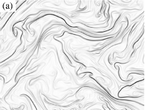
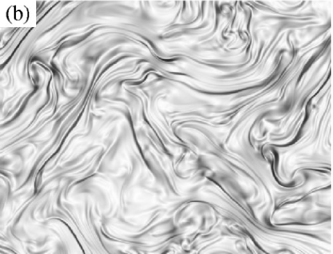
Figure 15: A snapshot of T-Vorticity and strain field. (a) a snapshot of T-Vorticity field, (b) that of strain field at the same location and time. Shading represents intensity of the field.

We introduce a vector quantity called T-Vorticity, $\bm{\chi}(\bm{x},t)$, as follows:

$$\bm{\chi}(\bm{x},t)=\left(\frac{\partial T}{\partial y},-\frac{\partial T}{\partial x}\right).$$ (41)

Figure 15 shows a snapshot of the magnitude of the T-Vorticity and the strain field. It is observed that there are linearly concentrated area of T-vorticity. Its width and length are an order of the entropy dissipation scale and the integral scale, respectively Toh and Matsumoto (2003). We call these fine coherent structures. At the same location of the structures, we can observe linearly straining regions in Fig. 15(b).

T-Vorticity has similar properties to vorticity in the 3D-NS turbulence. The evolution equation of the T-Vorticity has the stretching term and is the same as that of vorticity in 3D-NS system:

$$\frac{\partial\bm{\chi}}{\partial t}+(\bm{u}\cdot\nabla)\bm{\chi}=(\bm{\chi}\cdot\nabla)\bm{u}+\kappa\triangle\bm{\chi}.$$ (42)

Accordingly, there is a solution corresponding to the Burgers vortex in the 3D-NS system, which is called the Burgers T-vortex layer. It is numerically confirmed that fine coherent structures in the 2D-FC turbulence are well approximated by the Burgers T-vortex layer Toh and Matsumoto (2003). This is similar to fine coherent structures such as worms in the 3D-NS turbulence which are well approximated by the Burgers vortex.

Appendix B exit-time statistics

The exit-time statistics is one of the scale-fixed statistics. The exit-time, $T_{\mathrm{E}}(R;\rho)$, is defined as

$$T_{\mathrm{E}}(R;\rho)\equiv T_{\mathrm{F}}(\rho R)-T_{\mathrm{F}}(R),$$ (43)

where $T_{\mathrm{F}}(R)$ is the time when a relative separation $r(t)$ reach a threshold $R$ for the first time (first-passage time) Artale et al. (1997); Boffetta et al. (1999); Boffetta and Sokolov (2002a). According to the scaling law of the characteristic time, $T_{c}\propto r^{s}$, and the additivity of the mean, the form of the mean exit-time is expected as follows:

$$\langle T_{E}(R;\rho)\rangle=\check{C}_{E}(\rho^{s}-1)r^{s},$$ (44)

where $\check{C}_{E}$ is a constant depending on the system. In the case of the Bolgiano-Obukhov scaling, $\check{C}_{E}=C_{E}^{\mathrm{(BO)}}(\alpha g)^{-2/5}\epsilon_{\theta}^{-1/5}$, where $C_{E}^{\mathrm{(BO)}}$ is considered to be a non-dimensional universal constant.

The exit-time statistics has two advantages over usual fixed-time statistics:

1. The exit-time statistics can specify a spatial scale by choosing a threshold $R$. Therefore we can extract information of the inertial range if both $R$ and $\rho R$ are in the inertial range.

2. The interval between thresholds (the width for averaging) can be controlled by $\rho$. This means that we can control the degree of coarse graining of dispersion process.

In order to calculate exit-times, we prepare a set of thresholds $R_{n}=\rho^{n}R_{0}$, where $n$ is a positive integer, and record the time at which $r(t)$ reach $R_{n}$ for the first time for every particle pairs and every $n$. In the present work, we set $\rho$ to $1.1^{1/8}$ $(\approx 1.01)$ and $R_{0}$ to the grid size $\Delta x$.

If Palm’s equation, Eq. (3), describes relative dispersion well, from the equation we can calculate the probability density function (PDF) of exit-time $P_{E}(T_{E};R,\rho)$, which represents the probability density for a particle pair of which exit-time from $R$ to $\rho R$ is $T_{E}$, Boffetta and Sokolov (2002a). In the present case, to calculate the PDF, first we solve Eq. (3) with the initial condition

$$P(r,0)=\delta(r-R),$$ (45)

where the boundary conditions are the reflecting condition at $r=0$ and the absorbing condition at $r=\rho R$. And then, the PDF is obtained as the time derivative of the probability of $r(t)<\rho R$:

$$P_{E}(T_{E};R,\rho)=\left.-\frac{d}{dt}\int_{r<\rho R}P(r,t)dr\right|_{t=T_{E}}.$$ (46)

We have numerically calculated the PDF of exit-time by the above procedure and compared with the PDF obtained by our DNS.

References

- Batchelor (1950) G. K. Batchelor, Q. J. R. Meteorol. Soc. 76, 133 (1950).
- Monin and Yaglom (1975) A. S. Monin and A. M. Yaglom, Statistical Fluid Mechanics, vol. 2 (MIT Press, Cambridge, 1975).
- Fung and Vassilicos (1998) J. C. H. Fung and J. C. Vassilicos, Phys. Rev. E 57, 1677 (1998).
- Richardson (1926) L. F. Richardson, Proc. R. Soc. A 110, 709 (1926).
- Jullien et al. (1999) M. C. Jullien, J. Paret, and P. Tabeling, Phys. Rev. Lett. 82, 2872 (1999).
- Ott and Mann (2000) S. Ott and J. Mann, J. Fluid Mech. 422, 207 (2000).
- Ishihara and Kaneda (2002) T. Ishihara and Y. Kaneda, Phys. Fluids 14, L69 (2002).
- Boffetta and Sokolov (2002a) G. Boffetta and I. M. Sokolov, Phys. Fluids 14, 3224 (2002a).
- Boffetta and Sokolov (2002b) G. Boffetta and I. M. Sokolov, Phys. Rev. Lett. 88, 094501 (2002b).
- Goto and Vassilicos (2004) S. Goto and J. C. Vassilicos, New J. Phys. 6, 65 (2004).
- Rivera and Ecke (2005) M. K. Rivera and R. E. Ecke, Phys. Rev. Lett. 95, 194503 (2005).
- Sawford (2001) B. Sawford, Annu. Rev. Fluid Mech. 33, 289 (2001).
- Sokolov (1999) I. M. Sokolov, Phys. Rev. E 60, 5528 (1999).
- Sokolov et al. (2000) I. M. Sokolov, J. Klafter, and A. Blumen, Phys. Rev. E 61, 2717 (2000).
- Dávila and Vassilicos (2003) J. Dávila and J. C. Vassilicos, Phys. Rev. Lett. 91, 144501 (2003).
- Ogasawara and Toh (2005a) T. Ogasawara and S. Toh (2005a), nlin.CD/0510053.
- Toh and Suzuki (1994) S. Toh and E. Suzuki, Phys. Rev. Lett. 73, 1501 (1994).
- Toh and Matsumoto (2003) S. Toh and T. Matsumoto, Phys. Fluids 15, 3385 (2003).
- Artale et al. (1997) V. Artale, G. Boffetta, A. Celani, M. Cencini, and A. Vulpiani, Phys. Fluids 9, 3162 (1997).
- Boffetta et al. (1999) G. Boffetta, A. Celani, A. Crisanti, and A. Vulpiani, Phys. Rev. E 60, 6734 (1999).
- Batchelor (1952) G. K. Batchelor, Proc. R. Soc. London Ser. A 213, 349 (1952).
- Ogasawara and Toh (2005b) T. Ogasawara and S. Toh, in IUTAM Symposium on Elementary Vortices and Coherent Structures: Significance in Turbulence Dynamics, edited by S. Kida (Springer, Berlin, 2005b), p. 143, in press.