Discrete Nonlinear Schrödinger Equations with arbitrarily high order nonlinearities

Abstract

A class of discrete nonlinear Schrödinger equations with arbitrarily high order nonlinearities is introduced. These equations are derived from the same Hamiltonian using different Poisson brackets and include as particular cases the saturable discrete nonlinear Schrödinger equation and the Ablowitz-Ladik equation. As a common property, these equations possess three kinds of exact analytical stationary solutions for which the Peierls-Nabarro barrier is zero. Several properties of these solutions, including stability, discrete breathers and moving solutions, are investigated.

I Introduction

The discrete nonlinear Schrödinger (DNLS) equation appears ubiquitously KRB throughout modern science since it represents one of the simplest equations in which the combination of dispersive effects with a cubic nonlinearity leads to localized solutions of soliton type. Most notable is the role it plays in understanding the propagation of electromagnetic waves in glass fibers and other optical waveguides OP . More recently the DNLS has been used as a tight binding model for Bose-Einstein condensates in optical lattices ST ; ABDKS . From a physical point of view, it is of interest to study the effects of including high order nonlinear terms (higher than cubic) in the equation on discrete solitons. These terms appear in different physical contexts such as Bose gases with hard core interactions in the Tonks-Girardeau regime vignolo and low-dimensional Bose-Einstein condensates in which quintic nonlinearities in the nonlinear Schrödinger (NLS) equation are used to model three-body interactions AS05 . A self-focusing cubic-quintic NLS equation is also used in nonlinear optics as a model for photonic crystals photonic .

For the continuous NLS equation with attractive interaction it is well known that the higher order nonlinearities (higher than cubic) lead to the collapse in a finite time (blow up) if the norm exceeds a critical value, even in the one-dimensional case. The interplay between dimensionality and the order of nonlinearity has indeed been used in the past as a way to investigate collapse in low dimensional nonlinear systems berge . Although in a discrete NLS system true collapse cannot occur, due to the conservation of the norm, it may be possible that some of the features observed in the continuous NLS system about localized solutions may also exist at the discrete level. In particular, it is known that in the 1D continuous NLS equation with high order nonlinearity (for example quintic) there exists only one localized solution for each value of the norm (critical norm), the so called Townes soliton chiao , which separates collapsing and decaying solutions while being marginally stable against decay or collapse. In the presence of an external field, for example a periodic potential, it is possible to stabilize such solutions of continuous NLS with higher order nonlinearities against decay, extending the existence range of localized solutions from a single value of the norm to a whole interval. Since the discrete NLS can be viewed as a tight binding model of the continuous NLS with a periodic potential, it is of interest to investigate the existence of discrete, stable localized solutions when higher order nonlinearity are introduced in the DNLS.

The aim of this paper is twofold. Firstly, we introduce a general DNLS equation with arbitrary higher order nonlinearities which in the appropriate limits reduces to the integrable Ablowitz-Ladik (AL) equation AL and to the cubic DNLS with a saturable nonlinearity I . These two equations have the remarkable property that they possess different analytical stationary solutions, both periodic and localized (solitonic), which are exact to all orders of nonlinearity. These solutions exist for specific values of frequency and nonlinear parameters and have been shown to be stable under small perturbations. Secondly, we investigate the effects of higher order nonlinearity on the stability and mobility of localized solutions of a generalized DNLS. In particular, we compute the Peierls-Nabarro (PN) barrier and perform direct numerical integration to show the existence of moving solutions.

The plan of the paper is as follows. In Sec. II we first show that the AL model AL and the saturable DNLS model I can be obtained from the same Hamiltonian. In Sec. III we extend these ideas to Hamiltonians with arbitrary nonlinearity and obtain several higher order DNLS models. We then obtain a number of (time) stationary, spatially periodic as well as localized solutions. In Sec. IV we study the various properties of these solutions. In Sec. V we examine the question of the existence of moving solutions in DNLS models with higher order nonlinearities. Finally in Sec. VI we point out the possible implications of our results and some open problems.

II The model

In a classic paper, Ablowitz and Ladik AL showed that one of the variants of the DNLS equation given by

$$i\dot{\psi}_{n}+(1+|\psi_{n}|^{2})[\psi_{n+1}+\psi_{n-1}]-2\psi_{n}=0,$$ (1)

is integrable. In Ref. Salerno a model was proposed which in one limit goes over to the DNLS model while in the other limit it goes over to the integrable AL model. Recently, we were able to obtain exact periodic solutions of the DNLS equation with a saturable nonlinearity I

$$i\dot{\psi}_{n}+(\psi_{n+1}+\psi_{n-1}-2\psi_{n})+\frac{\nu|\psi_{n}|^{2}}{1+\mu|\psi_{n}|^{2}}\psi_{n}=0,$$ (2)

which is an established model for optical pulse propagation in various doped fibers fibers . In Eq. (2), $\psi_{n}$ is a complex valued “wave function” at site $n$, while $\nu$ and $\mu$ are real parameters.

We point out that the two equations, i.e. Eqs. (1) and (2) can both be derived from the same Hamiltonian $\cal H$ given by:

$${\cal H}=\sum_{n=1}^{N}\bigg{[}|\psi_{n}-\psi_{n+1}|^{2}-\frac{\nu}{\mu}|\psi_{n}|^{2}$$

$$+\frac{\nu}{\mu^{2}}\ln\left(1+\mu|\psi_{n}|^{2}\right)\bigg{]},$$ (3)

and the equation of motion in both cases is

$$i\dot{\psi}_{n}=[\psi_{n},\cal H]\,.$$ (4)

The difference in the equations of motion comes from a different definition of the Poisson bracket (PB) and consequently a different definition of the time derivative. The Poisson bracket structure in both the cases can be compactly written as

$$[U,V]=\sum_{n=1}^{N}(\frac{\partial U}{\partial\psi_{n}}\frac{\partial V}{\partial\psi_{n}^{*}}-\frac{\partial U}{\partial\psi_{n}^{*}}\frac{\partial V}{\partial\psi_{n}})(1+\lambda|\psi_{n}|^{2})\,.$$ (5)

On using Eqs. (3) and Eq. (4) for $\lambda=0$ ($\psi_{n}$ and $i\psi_{n}^{*}$ are conjugate variables) it yields Eq. (2) I through Eq. (4), while $\lambda=\mu$ ($\psi_{n}$ and $i\psi_{n}^{*}$ are non-conjugate variables) yields the equation introduced in Ref. Salerno

$$i\dot{\psi}_{n}+(1+\mu|\psi_{n}|^{2})(\psi_{n+1}+\psi_{n-1}-2\psi_{n})+\nu|\psi_{n}|^{2}\psi_{n}=0.$$ (6)

Notice that for $\mu\rightarrow 0$ both Eq. (2) and Eq. (6) reduce to the ordinary DNLS. Therefore, in the following we will assume $\mu\neq 0$ and perform the transformation $\sqrt{\mu}\psi_{n}\rightarrow\psi_{n}$. This will replace $\mu$ by 1 and $\frac{\nu}{\mu}$ by $\nu$, thus rendering the problem a one parameter problem.

For the $\lambda=0$ case I the equation of motion, Eq. (2), can be written as

$$i(1+|\psi_{n}|^{2})\dot{\psi}_{n}+(1+|\psi_{n}|^{2})(\psi_{n+1}+\psi_{n-1}-2\psi_{n})$$

$$+\nu|\psi_{n}|^{2}\psi_{n}=0,$$ (7)

while for the $\lambda=1(=\mu)$ Eq. (6) becomes:

$$i\dot{\psi}_{n}+(1+|\psi_{n}|^{2})(\psi_{n+1}+\psi_{n-1}-2\psi_{n})+\nu|\psi_{n}|^{2}\psi_{n}=0.$$ (8)

Note that $\nu=2$ in Eq. (8) gives the AL equation AL , Eq. (1).

In both cases a conserved power ${\cal P}$ can be written:

$${\cal P}=\sum_{n=1}^{N}\frac{1}{\lambda}\ln(1+\lambda|\psi_{n}|^{2})\,,~{}~{}\lambda\rightarrow 0~{}~{}\mbox{or}~{}~{}\lambda=\mu=1\,.$$ (9)

The difference between the two cases is the presence of $i|\psi_{n}|^{2}$ in the factor in front of the time derivative term in Eq. (7). However, for a stationary solution [i.e. only $\exp(-i\omega t)$ time dependence: $i\dot{\psi}_{n}=\omega\psi_{n}$] Eq. (7) can be written as

$$i\dot{\psi}_{n}+(1+|\psi_{n}|^{2})(\psi_{n+1}+\psi_{n-1}-2\psi_{n})$$

$$+(\nu+\omega)|\psi_{n}|^{2}\psi_{n}=0\,,$$ (10)

which is identical in form to Eq. (6).

The exact solutions to Eq. (7) given in I all are stationary solutions “rotating” with the frequency

$$\omega=2-\nu\,.$$ (11)

Inserting this frequency into Eq. (10) gives the AL equation:

$$i\dot{\psi}_{n}+(1+|\psi_{n}|^{2})(\psi_{n+1}+\psi_{n-1}-2\psi_{n})+2|\psi_{n}|^{2}\psi_{n}=0\,.$$ (12)

From this is clear that exact stationary solutions of the saturable DNLS equation I are also stationary solutions of the AL equation. Analytical expressions for stationary and moving solutions of the AL equation were given by Scharf and Bishop in Ref. Alan (note that their $\omega$ differs from ours by a factor of two, see Eq. (11). We also remark that, because of the frequency relation $\omega+\nu=2$, Eq. (6) has stationary solutions of the AL only if $\nu=2$, i.e. when it reduces to the AL equation. In the following we shall demonstrate the existence of analytical stationary solutions of the AL type also for generalizations of Eqs. (2), (6), with arbitrarily high order nonlinearities.

II.1 High order nonlinearities

We now generalize the nonlinear part of the Hamiltonian $\cal H$ in Eq. (3) by replacing $\ln(1+|\psi_{n}|^{2})$ by:

$$\ln(1+f(|\psi_{n}|^{2})),$$ (13)

where the function $f(x)$, a polynomial of degree $p+1$, is given by:

$$f(x)=\sum_{j=0}^{p}\alpha_{j}x^{j+1}.$$ (14)

Here $\alpha_{0}$ is always 1. Having already considered the case $\mu\rightarrow 0$, and having chosen $\mu=1$, we can next choose two different values of $\nu$ in Eq. (3). Therefore, instead of Eq. (3), the Hamiltonian ${\cal H}$ is now given by:

$${\cal H}=\sum_{n=1}^{N}\bigg{[}|\psi_{n}-\psi_{n+1}|^{2}-\nu^{\prime}|\psi_{n}|^{2}$$

$$+\nu\ln(1+f(|\psi_{n}|^{2}))\bigg{]},$$ (15)

and the generalized Poisson bracket by:

$$[U,V]=$$

$$\sum_{n=1}^{N}\left(\frac{dU}{d\psi_{n}}\frac{dV}{d\psi_{n}^{*}}-\frac{dV}{d\psi_{n}}\frac{dU}{d\psi_{n}^{*}}\right)\left[1+\lambda f(|\psi_{n}|^{2})\right],$$ (16)

with $\lambda=0$ or 1. Note that the equation of motion is still given by Eq. (4).

We notice for the $\lambda=0$ case that a transformation $\psi_{n}\rightarrow e^{-i\Delta\omega t}\psi_{n}$ would add $\Delta\omega$ to the coefficient of $\psi_{n}$ in the equation of motion and subtract the same from the coefficient of the $|\psi_{n}|^{2}$ term in the Hamiltonian. Therefore, a $\nu^{\prime}$ different from $\nu$ will only shift the frequency. We remark that some of the recently discussed models had fall in this category and are essentially equivalent to the saturated DNLS model I . Thus, both in this section and in Sec. IIIA the effect will only be to change the frequency $\omega$ by $\Delta\omega$. This will, however, not be the case for $\lambda=1$ as discussed here and in Sec. IIIB.

We also note that with higher order nonlinearities too, besides the Hamiltonian ${\cal H}$, the power

$${\cal P}=\sum_{n=1}^{N}|\psi_{n}|^{2}\,,~{}~{}\lambda=0\,,$$ (17)

or

$${\cal P}=\sum_{n=1}^{N}\ln(1+f(|\psi_{n}|^{2}))\,,~{}~{}\lambda=1\,,$$ (18)

is a conserved quantity.

III Exact analytical solutions

The main objective here is to find stationary solutions of the type obtained in Ref. I but with an additional amplitude factor $A$ in the equation of motion derived from the generalized Hamiltonian ${\cal H}$ given by Eq. (15). In particular, as in Ref. I we try to obtain three different types of solutions. The type I solution is given by

$$\psi_{n}^{I}=A\frac{\mbox{sn}(\beta,m)}{\mbox{cn}(\beta,m)}e^{-i(\omega t+\delta)}{\rm dn}(\beta(n+c),m)\,,$$ (19)

where the frequency $\omega$ is given by Eq. (11) while the two equations determining $m$ and $\beta$ are

$$\beta=\frac{2K(m)}{N_{p}}\,,~{}~{}\nu=2\frac{{\rm dn}(\beta,m)}{{\rm cn}^{2}(\beta,m)}\,.$$ (20)

Here $N_{p}$ denotes the number of sites in one period of the system. On the other hand, the type II solution is given by

$$\psi_{n}^{II}=A\sqrt{m}\frac{\mbox{sn}(\beta,m)}{\mbox{dn}(\beta,m)}e^{-i(\omega t+\delta)}{\rm cn}(\beta(n+c),m),$$ (21)

with the same frequency $\omega$ as given by Eq. (11) and the two equations determining $m$ and $\beta$ being:

$$\beta=\frac{4K(m)}{N_{p}}\,,~{}~{}\nu=2\frac{{\rm cn}(\beta,m)}{{\rm dn}^{2}(\beta,m)}\,,$$ (22)

Here, ${\rm sn}(x,m)$, ${\rm cn}(x,m)$, and ${\rm dn}(x,m)$ are the Jacobi elliptic functions of modulus $m$, while $K(m)$ is the complete elliptic integral of the first kind stegun . The two solutions have a common limit for $m\rightarrow 1$ giving the type III solution:

$$\psi_{n}^{III}=A\frac{\sinh(\beta)}{\cosh(\beta(n+c))}e^{-i(\omega t+\delta)},~{}(N_{p}\rightarrow\infty)\,,$$ (23)

with $\beta$ being determined by:

$$\nu=2\cosh(\beta)\,.$$ (24)

III.1 Standard Poisson brackets, $\lambda=0$

In this case of the standard PB ($\lambda=0$), the equation of motion becomes:

$$i\dot{\psi}_{n}+\left[\psi_{n+1}-2\psi_{n}+\psi_{n-1}\right]$$

$$+\frac{\nu^{\prime}(1+f(|\psi_{n}|^{2})-\nu f^{\prime}(|\psi_{n}|^{2}))}{(1+f(|\psi_{n}|^{2}))}\psi_{n}=0\,,$$ (25)

or equivalently,

$$(i\dot{\psi}_{n}-2\psi_{n}+\nu^{\prime}\psi_{n})(1+f(|\psi_{n}|^{2})$$

$$+\left[\psi_{n+1}+\psi_{n-1}\right](1+f(|\psi_{n}|^{2}))-\nu f^{\prime}(|\psi_{n}|^{2})\psi_{n}=0\,.$$ (26)

This equation has the stationary solutions of the form (Type I, II, and III) as given by Eqs. (19), (21), and (23) where the frequency $\omega$ is still given by Eq. (11) but with $\nu$ replaced by $\nu^{\prime}$:

$$\omega=2-\nu^{\prime}\,.$$ (27)

Also, the two equations needed to determine $m$ and $\beta$ are still the same. The condition on the amplitude is that $A=\sqrt{p+1}$ and that the coefficients of the polynomial $\alpha_{j}$ in Eq. (II.1) are given by

$$\alpha_{j}=\frac{p}{(j+1)!}\frac{\Pi_{k=1}^{j-1}(p-k)}{(p+1)^{j}},~{}~{}1\leq j\leq p\,.$$ (28)

This specifies the equation completely. We find:

$$1+f(x)=\left(1+\frac{x}{p+1}\right)^{p+1}~{}~{}\rightarrow e^{x}~{}\mbox{for}~{}p\rightarrow\infty~{}~{}.$$ (29)

For the first few values of $p$ one finds:

$$\begin{array}[]{lllll}p=1:&\alpha_{1}=\frac{1}{4},&{}&{}&{}\\ p=2:&\alpha_{1}=\frac{1}{3},&\alpha_{2}=\frac{1}{27},&{}&{}\\ p=3:&\alpha_{1}=\frac{3}{8},&\alpha_{2}=\frac{1}{16},&\alpha_{3}=\frac{1}{256},&{}\\ p=4:&\alpha_{1}=\frac{2}{5},&\alpha_{2}=\frac{2}{25},&\alpha_{3}=\frac{1}{125},&\alpha_{4}=\frac{1}{3125}.\\ \end{array}$$

We note that $p=0$ gives the results of Ref. I . We also note that the $p>0$ cases are just a rescaling of the results of Ref. I . Thus the higher order nonlinearities do not give anything essentially new in the $\lambda=0$ case.

III.2 Non-standard Poisson brackets, $\lambda=1$

This case of the non-standard PB represents a generalization of Eq. (6). From Eq. (4) and Eq. (16) we get

$$i\dot{\psi}_{n}+\left[\psi_{n+1}+\psi_{n-1}\right][1+f(|\psi_{n}|^{2})]$$

$$+(\nu^{\prime}-2)[1+f(|\psi_{n}|^{2})]\psi_{n}-\nu f^{\prime}(|\psi_{n}|^{2})\psi_{n}=0\,.$$ (30)

In order to use the identities for the Jacobi elliptic functions we must choose $\nu^{\prime}=2$, and we get a restricted generalization of Eq. (6)

$$i\dot{\psi}_{n}+\left[\psi_{n+1}+\psi_{n-1}\right][1+f(|\psi_{n}|^{2})]$$

$$-\nu f^{\prime}(|\psi_{n}|^{2})\psi_{n}=0\,.$$ (31)

This equation has the stationary solutions of the form (Type I, II, and III) as given by Eqs. (19), (21), and (23) except here the equations determining $m$ and $\beta$, are

$$\beta=\frac{2K(m)}{N_{p}}\,,~{}~{}\nu-\omega=2\frac{{\rm dn}(\beta,m)}{{\rm cn}^{2}(\beta,m)}\,$$ (32)

for the type I solutions,

$$\beta=\frac{4K(m)}{N_{p}}\,,~{}~{}\nu-\omega=2\frac{{\rm cn}(\beta,m)}{{\rm dn}^{2}(\beta,m)}\,$$ (33)

for type II, and finally

$$\nu-\omega=2\cosh(\beta)\,$$ (34)

for type III. The condition on the amplitude is now that $A=\sqrt{p+1}\sqrt{\frac{\nu}{\nu-\omega}}$ and that the coefficients of the polynomial $\alpha_{j}$ are given by

$$\alpha_{j}=\frac{1}{(j+1)!}\frac{\Pi_{k=1}^{j-1}(p-k)}{(p+1)^{j-1}}\left(\frac{\nu-\omega}{\nu}\right)^{j}\left(1-\frac{\nu-\omega}{\nu(p+1)}\right)\,,$$

$$1\leq j\leq p\,.$$ (35)

Note that the frequency $\omega$ now also appears as a parameter. This completely specifies our equation.

We find:

$$1+f(x)=\frac{1}{p}\left(\frac{\nu(p+1)}{\nu-\omega}-1\right)\left(1+\frac{\nu-\omega}{\nu}\frac{x}{p+1}\right)^{p+1}$$

$$-\frac{\omega}{\nu-\omega}\frac{p+1}{p}\left(1+\frac{\nu-\omega}{\nu}\frac{x}{p+1}\right)\,.$$ (36)

In addition, for $p\rightarrow\infty$

$$1+f(x)\rightarrow\frac{\nu}{\nu-\omega}e^{\frac{\nu-\omega}{\nu}x}-\frac{\omega}{\nu-\omega}\,,$$ (37)

and

$$f^{\prime}(x)\rightarrow e^{\frac{\nu-\omega}{\nu}x}\,.$$ (38)

For the first few values of $p$ we find:

$$\begin{array}[]{llll}p=1:&\alpha_{1}=\frac{\nu-\omega}{2\nu}(1-\frac{\nu-\omega}{2\nu}),&{}&\\ p=2:&\alpha_{1}=\frac{\nu-\omega}{2\nu}(1-\frac{\nu-\omega}{3\nu}),&\alpha_{2}=\frac{(\nu-\omega)2}{18\nu 2}(1-\frac{\nu-\omega}{3\nu}),&\\ p=3:&\alpha_{1}=\frac{\nu-\omega}{2\nu}(1-\frac{\nu-\omega}{4\nu}),&\alpha_{2}=\frac{(\nu-\omega)2}{12\nu 2}(1-\frac{\nu-\omega}{4\nu}),&\\ {}&\alpha_{3}=\frac{(\nu-\omega)3}{192\nu 3}(1-\frac{\nu-\omega}{4\nu}).\\ \end{array}$$

Note that if $\omega=0$ (i.e., $\frac{\nu-\omega}{\nu}=1$) then, as expected, $\alpha_{j}$ are the same in non-standard Poisson bracket case as in the standard Poisson bracket case. We would like to remind that if one also chooses $\nu=2$ then one obtains the AL model and its higher order generalizations.

It may be noted here that in order to obtain the above solutions we have made use of two identities for the Jacobi elliptic functions Khare . The first identity is

$${\rm dn}^{2}(x)[{\rm dn}(x+a)+{\rm dn}(x-a)]=A{\rm dn}(x)$$

$$+B[{\rm dn}(x+a)+{\rm dn}(x-a)]\,,$$ (39)

where

$$A=2{\rm ns}(a){\rm ds}(a)\,,~{}~{}B=-{\rm cs}^{2}(a)\,.$$ (40)

Here ${\rm ns}(a)\equiv\frac{1}{{\rm sn}(a)},{\rm ds}(a)\equiv\frac{{\rm dn}(a)}{{\rm sn}(a)},{\rm cs}(a)\equiv\frac{{\rm cn}(a)}{{\rm sn}(a)}$. We have suppressed the modulus $m$ in our notation here. On repeatedly multiplying both sides of the identity (III.2) by ${\rm dn}^{2}(x)$ and simplifying yields the following general identity of arbitrary (odd) rank:

$${\rm dn}^{2n}(x)[{\rm dn}(x+a)+{\rm dn}(x-a)]=B^{n}[{\rm dn}(x+a)$$

$$+{\rm dn}(x-a)]+A\sum_{j=1}^{n}B^{j-1}{\rm dn}^{2(n-j)+1}(x)\,,$$ (41)

which has been used in deriving some of the above solutions. Here $A$, $B$ are the same as given by Eq. (40).

The second identity we have used above is Khare

$$m{\rm cn}^{2}(x)[{\rm cn}(x+a)+{\rm cn}(x-a)]=A{\rm cn}(x)$$

$$+B[{\rm cn}(x+a)+{\rm cn}(x-a)]\,,$$ (42)

where

$$A=2{\rm ns}(a){\rm cs}(a)\,,~{}~{}B=-{\rm ds}^{2}(a)\,.$$ (43)

On repeatedly multiplying both sides of this identity by $m{\rm cn}^{2}(x)$ and simplifying yields the following general identity of arbitrary (odd) rank:

$$m^{n}{\rm cn}^{2n}(x)[{\rm cn}(x+a)+{\rm cn}(x-a)]=B^{n}[{\rm cn}(x+a)$$

$$+{\rm cn}(x-a)]+A\sum_{j=1}^{n}m^{n-j}B^{j-1}{\rm cn}^{2(n-j)+1}(x)\,,$$ (44)

which has been used in deriving some of the above solutions. Here $A$, $B$ are the same as given by Eq. (43).

III.3 The $p\rightarrow\infty$ limit and the linear limit

Both $\lambda=0$ and $\lambda=1$ cases have the same linear (small signal) limit:

$$i\dot{\psi}_{n}-(2+\nu-\nu^{\prime})\psi_{n}+(\psi_{n+1}+\psi_{n-1})=0.$$ (45)

For the $\lambda=0$ case, the $p\rightarrow\infty$ limit gives the same equation (45), because in this limit $1+f(x)=f^{\prime}(x)=e^{x}$. For the $\lambda=1$ case, however, $1+f(x)$ and $f^{\prime}(x)$ differ as is clear from Eqs. (37) and (38). Inserting these two equations into Eq. (31) yields

$$i\dot{\psi}_{n}-\omega\frac{\psi_{n+1}+\psi_{n-1}}{\nu-\omega}$$

$$+\nu e^{\frac{\nu-\omega}{\nu}x}\left(\frac{\psi_{n+1}+\psi_{n-1}}{\nu-\omega}-\psi_{n}\right)=0.$$ (46)

This equation is a little bit tricky since it contains terms of the order $\sqrt{p}$ and $\sqrt{p}e^{p}$. We must balance the $\sqrt{p}e^{p}$ terms first giving:

$$\psi_{n+1}+\psi_{n-1}=(\nu-\omega)\psi_{n},$$ (47)

and next balance the smaller terms giving

$$i\dot{\psi}_{n}=\omega\psi_{n}.$$ (48)

Note that in this case we end up with two coupled linear equations, one describing the spatial variation and one describing the temporal variation.

IV Properties of the New Solutions

IV.1 PN Barrier

In a discrete lattice there is an energy cost associated with moving localized modes (such as a soliton or a breather) by a half lattice constant. This is the celebrated Peierls-Nabarro (PN) barrier PN ; peyrard . As is well known, while for the AL (i.e. $p=0,\lambda=1,\nu=2$) case, this barrier is known to be zero, as shown by us in Ref. I , this barrier is nonzero in the case of the saturated DNLS model (i.e. $p=0$, $\lambda=0$). It is then of significant interest to know whether this barrier exists in models with higher order nonlinearities. Since for $p=0$, $\lambda=0$, we have already studied the various properties of the solutions in Ref. I and since higher order nonlinearities do not give anything essentially new, we will only study the properties of the $\lambda=1$ solutions. In particular, we will show that like the AL case, even for all the higher order models, the PN barrier is zero.

In view of $\nu^{\prime}=2$, the Hamiltonian (15) (for $\lambda=1$) takes a simple form

$${\cal H}=\sum_{n=1}^{N}\bigg{[}-\psi_{n}\psi_{n+1}^{*}-\psi_{n}^{*}\psi_{n+1}+\nu\ln(1+f(|\psi_{n}|^{2}))\bigg{]}$$

$$\equiv H_{1}+H_{2}\,,$$ (49)

while the power $P$ is as given by Eq. (18). The first part of the Hamiltonian without the logarithmic term ($H_{1}$) is easily evaluated in the case of all the three solutions as given by Eqs. (19), (21) and (23) and it is easily shown that for all the three solutions the answer is independent of the constant $c$, i.e., the distance from a lattice point where the center of the elliptic soliton solution is located. For example, for solution of type I, we obtain

$$H_{1}^{I}=-\frac{2A^{2}N_{p}}{{\rm cs}^{2}(\beta,m)}[{\rm dn}(\beta,m)-{\rm cs}(\beta,m)Z(\beta,m)]\,,$$ (50)

while for the solution of type II

$$H_{1}^{II}=-\frac{2A^{2}N_{p}}{{\rm cs}^{2}(\beta,m)}[m{\rm cn}(\beta,m)-{\rm ds}(\beta,m)Z(\beta,m)]\,,$$ (51)

and for solution of type III

$$H_{1}^{III}=-4A^{2}\sinh(\beta)\,.$$ (52)

Here $Z(\beta,m)$ is the Jacobi zeta function stegun . While deriving these relations, use has been made of the identities in Ref. Khare

$${\rm dn}(x){\rm dn}(x+a)={\rm dn}(a)-{\rm cs}(a)Z(a)+{\rm cs}(a)[Z(x+a)-Z(x)]\,,$$ (53)

$$m{\rm cn}(x){\rm cn}(x+a)=m{\rm cn}(a)-{\rm ds}(a)Z(a)$$

$$+{\rm ds}(a)[Z(x+a)-Z(x)]\,,$$ (54)

We are unable to evaluate the expression for power $P$ and (hence) the second term in the Hamiltonian $H_{2}$ analytically for any nonzero $p$ in the case of solutions of type I and II. However, this is easily accomplished in the case of the localized solutions (of type III). However, even without the explicit computation, it is easy to show that the PN barrier is zero in the case of all three solutions. Let us first explain the key idea. The power $P$ is given by

$$P=\sum_{n=1}^{N}\ln[1+\phi_{n}^{2}+\alpha_{1}\phi_{n}^{4}+...+\alpha_{p}\phi_{n}^{2p+2}]\,,$$ (55)

where $\psi_{n}=\phi_{n}e^{-i(\omega t+\delta)}$ and $\phi_{n}$ is easily obtained from Eqs. (19), (21) and (23). The key point to note is that the expression under the logarithm can always be factorized as

$$\left(1+\frac{\nu-\omega}{(p+1)\nu}\phi_{n}^{2}\right)\left[1+\frac{2\alpha_{1}\nu}{\nu-\omega}\phi_{n}^{2}+...+\frac{(p+1)\alpha_{p}\nu}{\nu-\omega}\phi_{n}^{2p}\right]\,,$$ (56)

which can be further factorized as

$$\left(1+\frac{\nu-\omega}{(p+1)\nu}\phi_{n}^{2}\right)[1+a_{1}\phi_{n}^{2}][1+a_{2}\phi_{n}^{2}]...[1+a_{p}\phi_{n}^{2}]\,,$$ (57)

where $a_{1},a_{2},...,a_{p}$ are the roots of the above equation. For example

$$\sum_{j=1}^{p}a_{j}=\frac{2\alpha_{1}\nu}{\nu-\omega}\,,~{}~{}\prod_{j=1}^{p}a_{j}=\frac{(p+1)\alpha_{p}\nu}{\nu-\omega}\,.$$ (58)

Hence the expression for power takes the simple form

$$P=\sum_{n=1}^{N}\ln\left[1+\frac{\nu-\omega}{(p+1)\nu}\phi^{2}\right]$$

$$+\sum_{j=1}^{p}\sum_{n=1}^{N}\ln[1+a_{j}\phi_{n}^{2}]\,.$$ (59)

We now observe that in the celebrated AL case, the power $P$ is given by

$$P=\sum_{n=1}^{N}\ln[1+\phi_{n}^{2}]\,,$$ (60)

where $\phi_{n}$ is either $a{\rm dn}[\beta(n+c-vt,m)]$ or ${\rm dn}$ replaced by ${\rm cn}[\beta(n+c-vt,m)]$ or by ${\rm sech}[\beta(n+c-vt)]$, and it is well known in that case that this sum is independent of $c$ since $P$ is a constant of motion and $t$ and $c$ always come together in this expression cai . As a result, it immediately follows that even for the higher order DNLS models the power $P$ and hence $H_{2}$ must also be $c$-independent being a sum of $p$ terms of the form same as that appears in the AL case. Thus we see that remarkably enough, even in higher order DNLS models the PN barrier is zero in the case of all three solutions.

Unfortunately for the solutions of type I and II we are unable to perform the additions analytically and hence compute $P$ and $H_{2}$ analytically. However, for the spatially localized solutions of type III this is easily accomplished. We observe that for the localized solutions of type III, each term in the sum has the form

$$\sum_{n=-\infty}^{\infty}\ln[1+a{\rm sech}^{2}\beta(n+c)]\,,$$ (61)

and as is well known from the AL case cai , this sum is $c$-independent and given by

$$\sum_{n=-\infty}^{\infty}\ln\left[1+a{\rm sech}^{2}\beta(n+c)\right]=\frac{2}{\beta}\left[\sinh^{-1}\sqrt{a}\right]^{2}\,.$$ (62)

Thus, in principle we know $P$ and $H_{2}$ for type III solutions. As an illustration, for the $p=1$ case, it is easily shown that

$$H_{2}=\nu P=2\beta\nu$$

$$+\frac{2\nu}{\beta}\bigg{[}\sinh^{-1}\left(\sqrt{\frac{2\nu}{\nu-\omega}[1-\frac{\nu-\omega}{2\nu}]}\sinh\beta\right)\bigg{]}^{2}\,.$$ (63)

Generalizing, for arbitrary $p$, the power P and $H_{2}$ are given by

$$H_{2}=\nu P+2\beta\nu$$

$$+\frac{2\nu}{\beta}\sum_{j=1}^{p}\left[\sinh^{-1}\left(\sqrt{(p+1)\frac{\nu}{\nu-\omega}a_{j}}\sinh\beta\right)\right]^{2}\,.$$ (64)

It is indeed remarkable that the PN barrier is not only zero for the AL model but for even higher order generalizations. It would be worthwhile to examine if the higher order models are also integrable, although perhaps the answer is likely not in the affirmative.

IV.2 Stability

In order to study the linear stability of the exact solutions $\psi_{n}^{j}$ ($j$ is I, II, or III) we introduce the following expansion

$$\psi_{n}(t)=\psi_{n}^{j}+\delta\psi_{n}(t)e^{-i\omega t},$$ (65)

applied in a frame rotating with frequency $\omega$ of the solution. The stability analysis for the $p=0,\lambda=0$ case was carried out in Ref. I and as seen above, higher order nonlinearities do not give any new solution. We will therefore only consider the stability of $\lambda=1$ solutions. Upon using this expansion into the equation of motion (for $\lambda=1,\nu^{\prime}=2$)

$$i\dot{\psi}_{n}+[\psi_{n+1}+\psi_{n-1}][1+f(|\psi_{n}|^{2})]$$

$$-\nu f^{\prime}(|\psi_{n}|^{2})\psi_{n}=0.$$ (66)

Next, retaining only terms linear in the perturbation, and taking into account the basic frequency $\omega$ of the unperturbed solutions and the perturbations, we get

$$i\delta\dot{\psi}_{n}+\big{(}\delta\psi_{n+1}+\delta\psi_{n-1}\big{)}[1+f(|\psi_{n}|^{2})]$$

$$+(\omega-\nu f^{\prime}(|\psi_{n}|^{2}))\delta\psi_{n}+\big{(}\psi_{n}^{*}(\psi_{n+1}+\psi_{n-1})f^{\prime}(|\psi_{n}|^{2})$$

$$-\nu f^{\prime\prime}(|\psi_{n}|^{2})|\psi_{n}|^{2}\big{)}(\delta\psi_{n}+\delta\psi_{n}^{*})=0.$$ (67)

Continuing by splitting the perturbation $\delta\psi_{n}$ into real parts $\delta u_{n}$ and imaginary parts $\delta v_{n}$ ($\delta\psi_{n}=\delta u_{n}+i\delta v_{n}$) and introducing the two real vectors

$$\delta\mbox{\boldmath$U$}=\{\delta u_{n}\} \delta\mbox{\boldmath$V$}=\{\delta v_{n}\}$$ and (68)

and the two real matrices $\mbox{\boldmath$A$}=\{A_{nm}\}$ and $\mbox{\boldmath$B$}=\{B_{nm}\}$ by defining

$$A_{nm}=[\delta_{n,m+1}+\delta_{n,m-1}][1+f(|\psi_{n}|^{2})]$$

$$+\bigg{(}\omega-\nu f^{\prime}(|\psi_{n}|^{2})-2\nu f^{\prime\prime}(|\psi_{n}|^{2})|\psi_{n}|^{2}$$

$$+2\psi_{n}^{*}[\psi_{n+1}+\psi_{n-1}]f^{\prime}(|\psi_{n}|^{2})\bigg{)}\delta_{nm}\,,$$

$$B_{nm}=[\delta_{n,m+1}+\delta_{n,m-1}][1+f(|\psi_{n}|^{2})]$$

$$+[\omega-\nu f^{\prime}(|\psi_{n}|^{2})]\delta_{nm}\,,$$ (69)

where $m\pm 1$ in the Kronecker $\delta$ means: $m\pm 1~{}mod~{}N$. Then Eq. (67) can be written compactly as

$$-\delta\mbox{\boldmath$\dot{V}$}+\mbox{\boldmath$A$}\delta\mbox{\boldmath$U$}=\mbox{\boldmath$0$}, \delta\mbox{\boldmath$\dot{U}$}+\mbox{\boldmath$B$}\delta\mbox{\boldmath$V$}=\mbox{\boldmath$0$},$$ and (70)

where an overdot denotes time derivative. Combining these first order differential equations we get:

$$\delta\mbox{\boldmath$\ddot{V}$}+\mbox{\boldmath$A$}\mbox{\boldmath$B$}\delta\mbox{\boldmath$V$}=\mbox{\boldmath$0$}, \delta\mbox{\boldmath$\ddot{U}$}+\mbox{\boldmath$B$}\mbox{\boldmath$A$}\delta\mbox{\boldmath$U$}=\mbox{\boldmath$0$}.$$ and (71)

The two matrices $A$ and $B$ are symmetric and have real elements. However, since they do not commute $A$$B$ and $\mbox{\boldmath$B$}\mbox{\boldmath$A$}=(\mbox{\boldmath$A$}\mbox{\boldmath$B$})^{T}$ ($T$ means transpose) are not symmetric. $A$$B$ and $B$$A$ have the same eigenvalues, but different eigenvectors. The eigenvectors for each of the two matrices need not be orthogonal. The eigenvalue spectrum $\{\gamma\}$ of the matrices $A$$B$ and $B$$A$ determines the stability of the exact solutions. If it contains negative eigenvalues, the solution is unstable. The eigenvalue spectrum always contains two eigenvalues which are zero. These eigenvalues correspond to the translational invariance ($c$) and to the invariance of the solution $\psi_{n}^{j}$ to a constant phase factor $e^{-i\delta}$ (i.e., translation in time), respectively.

In Fig.1 we show three examples of such stability evaluation. Figure 1 shows the lowest (non-zero) eigenvalue from the spectra of type III solutions obtained for $p=0$ (solid line) , $p=1$ (dashed line), and $p=2$ (dashed-dotted line). For the integrable AL case ($p=0$) we observe the expected result that all eigenvalues have a positive real value, indication that the exact solution is stable for all widths $\beta$. In contrast, we see that for both $p=1$ and $p=2$ the solution becomes unstable for certain values of $\beta$. This instability occurs for relatively large values of $\beta$, and thus when the solutions are very localized.

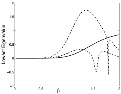
Figure 1: Lowest non zero-eigenvalues for type III solutions [Eq. (23)] for the (solid line) integrable AL equation (p=0), and for the nonintegrable cases of p=1 (dashed line), and p=2 (dashed-dotted line). For $p=1$ and $p=2$, the eigenvalues are observed to become negative, indicating instability, for certain values of $\beta$.

V Discrete breathers and moving solitons

In the following we focus on the AL limit of Eq. (31) and investigate the existence of localized stationary solutions, discrete breathers and moving excitations, by means of direct numerical integrations. In Fig. 2(a) we show the profiles of the localized states corresponding to the type III solution (soliton limit) for different values of $p$ and for the same parameter $\beta$ [notice that this parameter fixes the norm (power)]. We see that as $p$ is increased the amplitude (and the norm) of the solution increases as a consequence of the higher order nonlinearities. In panels (b), (c), and (d) of this figure we also show the time evolution of the stationary solutions for the cases $p=1,2,3$, respectively (similar results are obtained for higher values of p). Notice that the states are quite stable under time evolution, thus confirming the existence of stable localized solutions of the generalized Ablowitz-Ladik (GAL) equation with higher order nonlinearity.

Next we concentrate on moving solutions and on discrete breathers. To this end, we recall that for the case $p=0$ (i.e., the usual AL equation) exact moving solutions of the traveling waves type are well known Alan . One can show that an extension of these $p=0$ moving solutions to the case $p>0$ is not possible if one assumes a traveling wave ansatz.

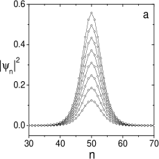
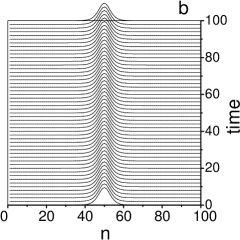
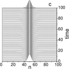
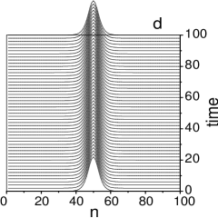
Figure 2: Panel (a). Stationary solutions of the GAL equation ($\nu=2$) for different values of $p$ ranging from $p=1$ (lower curve) to $p=8$ (upper curve). Other parameters are $\beta=0.25$, $m=1$. Panels (b), (c) and (d) show the time evolution of the solutions corresponding to the cases $p=1,2,3$, respectively.

The existence of a zero PN barrier, however, strongly suggests the existence of moving solutions for all values of $p$. In the following we investigate this aspect by means of a direct numerical experiment. In this context, let us consider initial conditions which are a linear superposition of two exact stationary solutions of the form

$$\psi(n,t) = Ae^{-i\omega t}\left[{\rm dn}[\beta(n-\frac{N}{2}+X_{0})]+\right.$$ (72)

$$\left.{\rm dn}[\beta(n-\frac{N}{2}-X_{0})]e^{-i\delta}\right],$$

with $A,\omega$ given by our previous formulas. By properly choosing the initial distance $2X_{0}$ between the centers of the humps (in order to have a weak overlap) we can bring them in interaction and at the same time have a good initial condition which is very close to an exact solution. As for the usual NLS solitons, the interaction between the humps depends on their distance and on their phase difference $\delta$. In particular, we have that the two humps attract each other if they are in phase ($\delta=0$) and repel if they are out of phase ($\delta=\pi$).

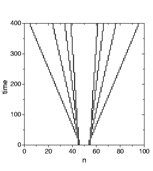
Figure 3: Time evolution of the position of the maxima of a two-hump solution of the GAL equation with $p=1$, $m=1$, originated from the initial condition in Eq. (72) with the distance between the two humps increased in steps of $1$ from $X_{0}=7$ (lower slopes) to $X_{0}=10$ (higher slopes). Other parameters are fixed as $\delta=\pi$, $\beta=1.25$.

The existence of a zero PN barrier can then be checked by increasing the initial distance between two out-of-phase humps and observe if the humps are set in motion by the mutual repulsion. Since by increasing the initial distance one considerably reduces the interaction between the humps (the interaction goes to zero exponentially with the distance) one has that for large separations motion can exist only if the PN barrier is zero. In Fig. 3 we show the results of such a numerical experiment by reporting the trajectories of the humps center (point of maximum amplitude) obtained from the GAL equation with $p=1$ (AL with cubic-quintic nonlinearity) for different values of $X_{0}$ and initial phase $\delta=\pi$. We see that for small initial separations the two humps move in opposite directions with high velocity while as we increase the initial separation the velocity gets progressively smaller. Our numerical investigations seem to indicate the absence of any critical threshold in the initial separation above which motion is stopped, which being in agreement with our analytical considerations about the absence of the PN barrier.

This behavior is also seen from Fig. 4(a) in which the time evolution of two stationary solutions of the GAL for $p=1$, initially displaced by a distance larger than their rest widths, is depicted. From this figure it is clear that there is practically no radiation generated during the motion, thus making the hump dynamics very close to that of exact (traveling wave) solitons. In panel (b) of this figure we depict the time dependence of the amplitude during the hump motion of panel (a), from which we observe that, except for the initial part where interaction dominates, a very regular pattern is generated. Notice that the amplitude oscillation lobes correspond to the vertical segments visible in the trajectories depicted in Fig. 3, the minima of the lobes corresponding to the times at which the maximum of the profile moves by one lattice site (i.e., to next vertical segment in the trajectory plot). From this we infer that the reciprocal of the period of the oscillation in the hump amplitude is just the hump velocity in lattice site units.

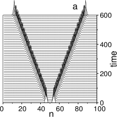
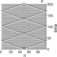
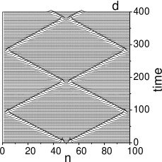
Figure 4: Panel (a). Time evolution of two solitons of the GAL equation obtained for $p=1$, $m=1$ and initial condition taken as in Eq. 72 with $X_{0}=4$. Other parameters are fixed as $\delta=\pi$, $\beta=1.25$. Panel (b). Time dependence of the humps amplitude (modulo square of the maximum of the profiles) depicted in the left panel. The minima correspond to the times at which the amplitude moves to the next lattice site. Parameters are the same as for panel (a). Panel (c). Time evolution of Eq. (31) with $p=1$, $N=100$ and initial condition taken as in Eq. (72) with $X_{0}=1$, $m=1$, $\beta=1.25$ and $\delta=\pi$. Panel (d). Same as in panel (c) but for $p=2$ and $X_{0}=3$.

It is remarkable that the absence of radiation in the hump dynamics is observed also for very long times and can survive multiple reflections. This is shown in panel (c) of Fig. 4 where the dynamics of two humps moving with a higher velocity (the velocity is increased by reducing the initial separation) is depicted. Notice that the humps undergo several collisions with almost no radiation generated. This behavior is a direct consequence of the zero PN barrier and is reminiscent of their soliton behavior. In panel (d) of Fig. 4 we show the same type of behavior for the case $p=2$. This result indicates that moving localized states of the GAL equation may exist also for higher values of $p$ (the stability of these solutions, however, may become critical as $p$ is increased).

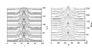
Figure 5: Left panel. Time evolution of Eq. (31) with $p=1$, $N=100$ and initial condition taken as in Eq. (72) with $X_{0}=5$, $m=1$, $\beta=0.15$ and $\delta=0$. Right panel. Same as for the left panel but for $p=2$ and $X_{0}=8$.

The existence of a zero PN barrier makes it also possible to have discrete breathers in the GAL equation. In order to show this we repeat the same type of experiments considered above but with an attractive instead of a repulsive interaction, i.e. we take the initial humps to be in phase instead of out of phase.

In Fig. 5 we depict the dynamics of two stationary solutions of the GAL equation for $p=1$ and with a small value of $\beta$ so that the initial profiles are very wide and have a large overlap. We see that, due to the mutual attraction, the two localized solutions undergo breathing oscillations with apparently no radiation generated. Notice that the norm, which is fixed by the parameter $\beta$, is below the instability threshold and the oscillations continue forever. This solution represents therefore an almost exact discrete breather of the GAL equation with higher order nonlinearity. In the right panel of Fig. 5 we show a discrete breather for the case $p=2$, indicating that these solutions may also exist with higher order nonlinearities. By increasing the norm or by increasing $p$, however, we find that an instability in the dynamics may develop at later times and the solution may become unstable. A preliminary investigation indicates the existence of a critical threshold (which depends on $p$) below which stable stationary humps and discrete breathers are stable. This stability threshold may be reminiscent of the collapse threshold that exists in the continuous NLS with higher order nonlinearities, for norms (powers) exceeding a critical value. For most physical applications, however, only the lowest higher order nonlinearities will be of interest (i.e., the cases p=1,2). In these cases stable discrete soliton-like and discrete breather solutions are found to be stable for a wide range of parameters (which one should be able to check with linear stability analysis).

We remark that the absence of the PN barrier, the presence of discrete breathers and the absence of emitted radiation during the hump dynamics could indicate a possible complete integrability of the GAL equation. Although this cannot be concluded without further analysis, we remark that the vanishing of the PN barrier is a necessary but not a sufficient condition for integrability. In this context we remark that for the nonintegrable discrete $\phi^{4}$ models oxtoby and for discrete sine-Gordon chains zolo it is possible to have a zero PN barrier and radiationless moving kinks for particular values of parameters. The GAL equation could possibly be another example in which this phenomenon may occur.

VI Conclusions

We have introduced a class of discrete nonlinear Schrödinger equations with arbitrarily high order nonlinearities which include as particular cases the saturable discrete nonlinear Schrödinger equation and the AL equation. We have obtained three different types of exact solutions (both spatially periodic in terms of Jacobi elliptic functions and their limiting hyperbolic case) for these models as well as that of a higher order generalization of the saturable discrete nonlinear Schrödinger equation and the Ablowitz-Ladik equation. We then studied the Peierls-Nabarro barrier PN ; peyrard for these solutions in various models and found that it is zero indicating that the soliton-like solutions move without experiencing any effect of the underlying discreteness, which is quite remarkable. We also studied the stability of these solutions under small perturbation and found that they are robust as well as stable. Finally, we investigated the collision of two hump solutions (both in-phase and out-of-phase cases) and found that they collide and move without any radiation. The out-of phase case indicates the formation of discrete breathers. These results are strongly suggestive of the integrability of the models introduced here, although we did not attempt to prove this rigorously. Our solutions and related properties are likely to be useful in many physical contexts including optical waveguides OP , Bose-Einstein condensates in optical lattices ST ; ABDKS , and nonlinear optics in the context of photonic crystals photonic .

VII Acknowledgments

AK and MRS acknowledge the hospitality of the Center for Nonlinear Studies and the Theoretical Division at Los Alamos. MS wishes to acknowledge partial financial support from a MURST-PRIN-2005 Initiative and the Department of Physics of The Technical University of Denmark, Lyngby, for the hospitality. This work was supported in part by the U.S. Department of Energy.

References

- (1) P.G. Kevrekidis, K.Ø. Rasmussen, and A.R. Bishop, Int. J. Mod. Phys. B 15, 2833, (2001).
- (2) H.S. Eisenberg, Y. Silberberg, R. Morandotti, A.R. Boyd, and J.S. Aitchison, Phys. Rev. Lett. 81, 3383 (1998).
- (3) A. Trombettoni and A. Smerzi, Phys. Rev. Lett. 86, 2353 (2001).
- (4) F.Kh. Abdullaev, B.B. Baizakov, S.A. Darmanyan, V.V. Konotop, and M. Salerno, Phys. Rev. A. 64, 043606 (2001).
- (5) A. Minguzzi, P. Vignolo, M.L. Chiofalo, and M. P. Tosi, Phys. Rev. A. 64, 033605 (2001); B. Damski, J. Phys. B 37, L85 (2004).
- (6) F.Kh. Abdullaev and M. Salerno, Phys. Rev. A. 72, 033617 (2005).
- (7) K.I. Maruno, Y. Ohta, and N. Joshi, Phys. Lett. A 311, 214 (2003).
- (8) L. Berge, Phys. Rep. 303, 259 (1998).
- (9) R.I. Chiao, E. Garmire, and C.H. Townes, Phys. Rev. Lett. 13, 479 (1964).
- (10) M.J. Ablowitz and J.F. Ladik, J. Math. Phys. 17, 1011 (1976).
- (11) M. Salerno, Phys. Rev. A 46, 6856 (1992).
- (12) A. Khare, K. Ø. Rasmussen, M.R. Samuelsen, and A. Saxena, J. Phys. A: Math. Gen. 38, 807 (2005).
- (13) S. Gatz and J. Herrmann, J. Opt. Soc. Am. B 8, 2296 (1991); S. Gatz and J. Herrmann, Opt. Lett. 17, 484 (1992).
- (14) Rainer Scharf and A.R. Bishop, Phys. Rev. A 43, 6535 ( 1991).
- (15) L. Hadzievski, A. Maluckov, M. Stepic, and D. Kip, Phys. Rev. Letters 93 (2004) 033901; M. Stepic, D. Kip, L. Hadzievski and A. Maluckov, Phys. Rev. E 69 (2004) 066618; J. Cuevas and J.C. Eilbeck, nlin.PS/0501050.
- (16) Handbook of Mathematical Functions with Formulas, Graphs, and Mathematical Tables, edited by M. Abramowitz and I. A. Stegun (U.S. GPO, Washington, D.C., 1964).
- (17) A. Khare and U. Sukhatme, J. Math. Phys. 43, 3798 (2002); A. Khare, A. Lakshminarayan, and U. Sukhatme, J. Math. Phys. 44, 1822 (2003); math-ph/0306028; Pramana (Journal of Physics) 62, 1201 (2004). (1991); J. P. Boyd, SIAM J. Appl. Math. 44, 952 (1984).
- (18) O. M. Braun and Yu. S. Kivshar, Phys. Rev. B 43, 1060
- (19) T. Dauxois and M. Peyrard, Phys. Rev. Lett. 70, 3935 (1993).
- (20) S. David Cai, Ph.D. Thesis, Northwestern University, Evanstan, IL (1994).
- (21) O.F. Oxtoby, D.E. Pelinovsky, and I.V. Barashenkov, Nonlinearity, 19 (2006) 217-235.
- (22) J.M. Speight and Y. Zolotaryuk, arXiv:nlin. PS/0509047.