A normal form for excitable media

We present a normal form for travelling waves in one-dimensional excitable media in form of a differential delay equation. The normal form is built around the well-known saddle-node bifurcation generically present in excitable media. Finite wavelength effects are captured by a delay. The normal form describes the behaviour of single pulses in a periodic domain and also the richer behaviour of wave trains. The normal form exhibits a symmetry preserving Hopf bifurcation which may coalesce with the saddle-node in a Bogdanov-Takens point, and a symmetry breaking spatially inhomogeneous pitchfork bifurcation. We verify the existence of these bifurcations in numerical simulations. The parameters of the normal form are determined and its predictions are tested against numerical simulations of partial differential equation models of excitable media with good agreement.

Excitable media are often found in biological and chemical systems. Examples of excitable media include electrical waves in cardiac and nerval tissue [1, 2], cAMP waves in slime mold aggregation [3] and intracellular calcium waves [4]. Excitable media support localized pulses and periodic wave trains. In 2 dimensions rotating vortices (or spirals) and in 3 dimensions scroll waves [5, 6, 7, 8, 9] are possible. The critical behaviour of pulses, wave trains and spirals, i.e. propagation failure, is often associated with clinical situations. The study of spiral waves is particularly important as they are believed to be responsible for pathological cardiac arrhythmias [10]. Spiral waves may be created in the heart through inhomogeneities in the cardiac tissue. Some aspects of spiral wave break up can be studied by looking at a one-dimensional slice of a spiral i.e. at a one-dimensional wave train [11].
We investigate critical behaviour relating to one-dimensional wave propagation. We develop a normal form which allows us to study the bifurcation behaviour of critical waves. In particular, the normal form predicts a Hopf bifurcation and a symmetry breaking pitchfork bifurcation. The symmetry breaking pitchfork bifurcation can be numerically observed as an instability where every second pulse of a wave train dies. This seems to be related to alternans [12, 13], which are discussed in the context of cardiac electric pulse propagation.

1 Introduction

Many chemical and biological systems exhibit excitability. In small (zero-dimensional) geometry they show threshold behaviour, i.e. small perturbations immediately decay, whereas sufficiently large perturbations decay only after a large excursion. This behaviour is crucial for the electrical activation of cardiac tissue or the propagation of nerve pulses where activation should only be possible after a sufficiently large stimulus. Moreover, the decay to the rest state allows for the medium to be repeatedly activated - also crucial for the physiological functioning of the heart and the nervous system. One-dimensional excitable media support travelling pulses, or rather, periodic wave trains ranging in wavelength $L$ from the localized limit $L\to\infty$ to a minimal value $L_{c}$ below which propagation fails. Pulses and wave trains are best-known from nerve propagation along axons. In two dimensions one typically observes spiral waves. Spirals have been observed for example in the auto-catalytic Belousov-Zhabotinsky reaction [5], in the aggregation of the slime mold dictyostelium discoideum [3] and in cardiac tissue [2].

For certain system parameters the propagation of isolated pulses and wave trains may fail (see for example [14, 15]). The analytical tools employed to describe these phenomena range from kinematic theory [16, 17], asymptotic perturbation theory [18, 19, 20] to dynamical systems approaches [21, 22, 23]. Numerical observations reveal that independent of the detailed structure of a particular excitable media model, the bifurcation behaviour of excitable media is generic. For example, a saddle-node bifurcation is generic for single pulses and for wave trains. However, there exists no general theory which accounts for all bifurcations which may appear. In this paper we develop a normal form for excitable media which is build around the observation that the propagation failure of a one-dimensional wave train is mediated by the interaction of a pulse with the inhibitor of the preceding pulse.

In Section 2 we briefly review some basic properties of excitable media and illustrate them with a specific example. In Section 3 we introduce the normal form. The properties and the bifurcation scenarios of this normal form are investigated in Section 4. In Section 5 we show how the parameters of the normal form can be determined from numerical simulations of the excitable medium and then compare the predictions of the normal form with actual numerical simulations of a partial differential equation. The paper concludes with a discussion in Section 6.

2 One-dimensional excitable media

Most theoretical investigations of excitable media are based on coupled reaction-diffusion models. We follow this tradition and investigate a two-component excitable medium with an activator $u$ and a non-diffusive inhibitor $v$ described by

$$\partial_{t}u = Du_{xx}+{\cal{F}}(u,v),\quad{\cal{F}}(u,v)=u(1-u)(u-u_{s}-v)$$

$$\partial_{t}v = \epsilon\ (u-a\ v)\ .$$ (1)

This is a reparametrized version of a model introduced by Barkley [24]. Note that the diffusion constant $D$ is not a relevant parameter as it can be scaled out by rescaling length. Although the normal form which we will introduce in Section 3 is independent of the particular model used, we illustrate some basic properties of excitable media using the particular model (2). Later in Section 5 we show correspondence of the predictions of our normal form with numerical simulations of the model (2). Our choice of model is motivated by the fact that this model incorporates the ingredients of an excitable system in a compact and lucid way. Thus, for $u_{s}>0$ the rest state $u_{0}=v_{0}=0$ is linearly stable with decay rates $\sigma_{1}=u_{s}$ along the activator direction and $\sigma_{2}=\epsilon a$ along the inhibitor direction. Perturbing $u$ above the threshold $u_{s}$ (in 0D) will lead to growth of $u$. In the absence of $v$ the activator would saturate at $u=1$ leading to a bistable system. A positive inhibitor growth factor $\epsilon$ and $a>0$ forces the activator to decay back to $u=0$. Finally also the inhibitor with the refractory time constant $(\epsilon\ a)^{-1}$ will decay back to $v=0$. For $a>1/(1-u_{s})$ the system is in zero-dimensional systems no longer excitable but instead bistable.

In order to study pulse propagation in one-dimensional excitable media it is useful to first consider the case of constant $v$. The resulting bistable model is exactly solvable [25] and the pulse velocity is $c_{f}(v)=\sqrt{\frac{D}{2}}[1-2(u_{s}+v)]$. Hence, excitability requires that $u_{s}$ is below the stall value $\frac{1}{2}$. The quantity $\Delta=\frac{1}{2}-u_{s}$ characterizes the strength of excitability and $c_{f}(0)$ coincides with the solitary pulse velocity for $\epsilon\to 0$.

Clearly, for $u_{s}<u_{c}=\frac{1}{2}$ and not too large $a$, pulse propagation fails for $\epsilon$ larger than some $\epsilon_{c}$. The critical growth factor $\epsilon_{c}$ marks the onset of a saddle-node bifurcation [16, 18, 23]. The saddle-node can be intuitively understood when we consider the activator pulse as a heat source, not unlike a fire-front in a bushfire. Due to the inhibitor the width of the pulse decreases with increasing $\epsilon$. Hence, the heat contained within the pulse decreases. At a critical width, or critical $\epsilon$, the heat contained within the pulse is too small to ignite/excite the medium in front of the pulse.

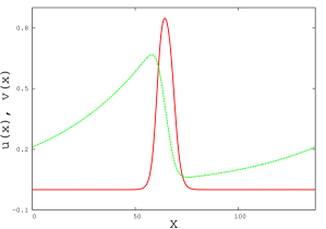
(a)

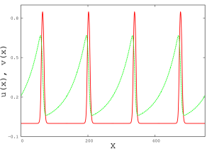
(b)

Figure 1: Typical profiles of the activator $u$ (continuous line) and inhibitor $v$ of close-to-critical travelling wave solutions in a one-dimensional ring of (2). Parameters are $a=0.22,u_{s}=0.1,\epsilon=0.035$. (a) Single pulse with $L=137.5$. (b) Wave train with $L=550$.

Even if a given set of equation parameters allows for propagation of a single isolated pulse, the system may not necessarily support a pulse in a periodic box of finite length or a wave train consisting of several of such pulses: If the distance $L$ between two consecutive pulses of the train becomes too small, the pulses run into the refractory tail of the preceding pulse (see Figure 1), and may consecutively decay . Hence, propagation failure for periodic wave trains is controlled by the decay of the inhibitor, and propagation is only possible when the inter-pulse distance $L$ is larger than a critical wavelength $L_{c}$. Note that $L_{c}$ diverges for $a\to 0$ when the decay rate of the inhibitor $\sigma_{2}$ vanishes. The critical wavelength $L_{c}$ is a lower bound for the wavelength for the existence of periodic wave trains. One can also think of keeping $L$ fixed and, as before, vary $\epsilon$. Then the saddle-node $\epsilon_{c}(L)$ is a monotonically increasing function.

In the next Section we present a normal form which incorporates the saddle-node bifurcation, and moreover predicts other types of bifurcations.

3 The normal form

It is well known that an isolated pulse undergoes a saddle-node bifurcation above a certain threshold value of the refractoriness $\epsilon_{c}$. The corresponding generic normal form for such a saddle-node bifurcation is given by

$$\partial_{t}X=-\mu-gX^{2}\;,$$ (2)

where $X$ is, for example, the amplitude or velocity of a pulse with the corresponding values at the saddle-node bifurcation subtracted. The bifurcation parameter $\mu$ measures the distance from the bifurcation point and is proportional to $\epsilon-\epsilon_{c}$. The normal form (2) accurately describes the behaviour of isolated solitary pulses in one-dimensional excitable media close to criticality. We use this normal form for a saddle-node bifurcation for an isolated pulse (2) as a seed to construct a normal form for general travelling in excitable media incorporating finite wavelength effects.

In particular we look at a single pulse on a ring with finite length, i.e. in a one-dimensional box with periodic boundary conditions, and at wave trains with a finite wavelength. Both cases are depicted in Figure 1. In that case the saddle-node (2) will be disturbed and will depend on the length of the periodic box in the case of a single pulse (Figure 1a) or on the wavelength of the wave train (Figure 1b). The interaction of the pulse (or a member of a wave train) with the preceding pulse (or more accurate with its inhibitor; see Figure 1) modifies as discussed above the bifurcation behaviour. We may therefore extend the saddle-node normal form to

$$\partial_{t}X=-\mu-gX^{2}-\beta_{0}V(t-\tau)\;,$$

where $V(t-\tau)$ describes the inhibitor of the preceding pulse who is temporally displaced by $\tau=L/c_{0}$ where $L$ is the wavelength of the pulse train, i.e. the distance between two consecutive pulses, and $c_{0}$ is its uniform velocity. We neglect here a possible temporal dependency of $\tau$. Note that in the case of a single pulse in a ring, $V(t-\tau)$ describes the inhibitor of the single pulse which had been created by the pulse at the time of the last revolution around the ring and $L$ is simply the length of the periodic box.
We assume an exponential decay (in space and time) of the inhibitor of well separated pulses. This is the case for the system (2). We may write $V(t-\tau)=\exp(-k\tau)h(X(t-\tau))$ where the function $h$ and the decay-rate $k$ depend on the particular model chosen; for example for the model (2) we have $k=\epsilon a$. In the limiting case of isolated pulses we note that $\tau\rightarrow\infty$ and $V(t-\tau)\rightarrow 0$, and hence we retrieve the unperturbed saddle-node bifurcation (2). The ansatz for $V(t-\tau)$ is a simplification where we ignore the cumulative effect of the inhibitor. (Note that the equation for the inhibitor $v$ in (2) can be solved directly and involves an integral over $u$, i.e. involves ’history’.) The unknown function $h(X(t-\tau))$ can be Taylor-expanded around the saddle-node $X=0$.

We summarize and arrive at the following normal form

$$\partial_{t}X=-\mu-gX^{2}-\beta(\gamma+X(t-\tau))\;,$$

where $\beta=\beta_{0}\exp(-k\tau)$ with $k=\epsilon a$ for the model equation (2). Pulses have a nonzero width $\nu$ which implies that the temporal delay $\tau=L/c_{0}$ has to be modified to $\tau=(L-\nu)/c_{0}$. This equation already produces qualitatively all the results we will present in the subsequent Sections. However, much better quantitative agreement is achieved by taking into account that a variation in the amplitude implies a change in velocities and henceforth a change of the effective inhibition. If we allow for a single pulse to have a temporarily varying pulse amplitude or, in the case of a wave train consisting of distinct members, if we allow for different amplitudes of individual members of the wave train, we have to take into account that the propagation behaviour is amplitude dependent: Larger pulses have larger velocities. Hence, a pulse $X(t)$ which is larger than its predecessor $X(t-\tau)$ runs further into the inhibitor-populated space created by its predecessor. If $X(t-\tau)<X(t)$ the finite wavelength induced shift of the bifurcation is stronger compared to the case of equal amplitudes. Conversely, if $X(t-\tau)>X(t)$ the finite wavelength induced shift of the bifurcation is weaker compared to the case of equal amplitudes. This effect is stronger the larger the difference of the two amplitudes $X(t-\tau)-X(t)$. The inclusion of the amplitude differences affects the bifurcation behaviour depending continuously on the difference $X(t-\tau)-X(t)$. We thus add a term $\gamma_{1}(X(t)-X(t-\tau))$ with $0<\gamma_{1}\ll 1$ into the wavelength dependant inhibitor term in (3), and arrive at

$$\partial_{t}X=-\mu-gX^{2}-\beta(\gamma+(1-\gamma_{1})X(t-\tau)+\gamma_{1}X(t))\;,$$

or after relabeling of $\beta,\gamma,\gamma_{1}$

$$\partial_{t}X=-\mu-gX^{2}-\beta(\gamma+X(t-\tau)+\gamma_{1}X(t))\;.$$ (3)

It is this equation which we propose as a normal form to study bifurcations of one-dimensional wave trains.

4 Properties of the normal form

Before we show how to determine the parameters of the normal form, we will describe its properties with a main emphasis on bifurcations. Besides the well-known saddle-node bifurcation we identify a symmetry preserving Hopf bifurcation and a symmetry breaking spatially inhomogeneous pitchfork bifurcation. Numerical integration of partial differential equation models of excitable media such as (2) confirm these bifurcation scenarios of the normal form (3). Although some of these bifurcations have been previously observed in numerical simulations, up to now there did not exist a unified framework to study these bifurcations. The normal form is able to identify these bifurcations as being generic for excitable media, rather than as being particular to certain models of excitable media. This is the main achievement of our present work.

4.1 Saddle-node bifurcation

Numerical simulations of excitable media show that the bifurcations of a single propagating pulse in a ring (as in Figure 1a) are different from the bifurcations of a wave train consisting of several distinct pulses (as in Figure 1b). We first look at a single propagating pulse before in Section 4.4 we look at the interaction of different pulses in a wave train.

Equation (3) has the following stationary solutions

$${\bar{X}}_{1,2}=\frac{1}{2g}[-\beta(1+\gamma_{1})\pm\sqrt{\beta^{2}(1+\gamma_{1})^{2}-4g(\mu+\beta\gamma)}]\;.$$ (4)

The upper solution branch is stable whereas the lower one is unstable. The two solutions coalesce in a saddle-node bifurcation with

$${\bar{X}}_{SN}=-\frac{\beta}{2g}(1+\gamma_{1})\quad{\rm{at}}\quad{\bar{\mu}}_{SN}=\frac{\beta^{2}}{4g}(1+\gamma_{1})^{2}-\beta\gamma\;.$$ (5)

Since $\beta=\beta_{0}\exp(-\epsilon a\tau)$ is small we have $\mu_{SN}<0$. This indicates that the saddle-node of a periodic wave train occurs at smaller values of the bifurcation parameter $\mu$ than for the isolated pulse, and the bifurcation is shifted to the left with respect to the isolated pulse (see Figure 3). This is a well known fact which we numerically verified. Note that the limiting case of an isolated pulses with $L\to\infty$ implies $\tau=0$ and hence, $\beta=0$. The saddle-node of the isolated pulse with $X_{SN}=0$ at $\mu=0$ described by (2) is recovered.

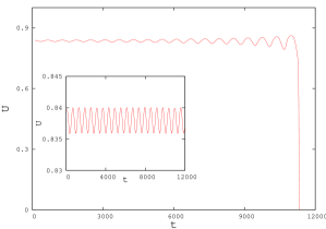
Figure 2: Temporal behaviour of the maximal amplitude $U$ of the activator $u$ for model (2) just above the subcritical Hopf bifurcation. The parameters are $\epsilon=0.3755$ and $L=246$. The other parameters are as in Figure 1. The subcritical character of the Hopf bifurcation is clearly seen at this length. If the length $L$ is chosen to be slightly larger and closer to the actual bifurcation point, the oscillations appear to be stable for some time as shown in the inset for $L=246.9695>L_{c}$. However, the maximal amplitude $U$ for $L=246.9695$ will eventually become visibly unstable and the pulse will die resulting in $U=0$.

Besides this stationary instability the normal form (3) also allows for a non-stationary bifurcation which we investigate in the next Section.

4.2 Symmetry preserving Hopf bifurcation

The stability of the homogeneous solution ${\bar{X}}$ with respect to small perturbations of the form $\delta X\exp{\sigma t}$ can be studied by linearizing the normal form around ${\bar{X}}$. We obtain

$$\sigma+2g{\bar{X}}+\beta\gamma_{1}+\beta e^{-\sigma\tau}=0\;.$$ (6)

Besides the stationary saddle-node bifurcation (5) at $\sigma=0$ (cf. (5)), a Hopf bifurcation $\sigma=i\omega$ is possible with

$$\omega = \beta\sin{\omega\tau}$$ (7)

$${\bar{X}}_{HH} = -\frac{\beta}{2g}(\cos{\omega\tau}+\gamma_{1})\;.$$ (8)

In anticipation of the study of wave trains consisting of several distinct pulses we call this Hopf bifurcation of a single pulse in a ring a symmetry preserving Hopf bifurcation. From (7) we infer that a Hopf bifurcation is only possible provided $\beta\tau>1$, i.e. if the coupling is strong enough and the pulse feels the presence of the inhibitor of the preceding pulse sufficiently strong. Since ${\bar{X}}_{HH}\geq{\bar{X}}_{SN}$ the symmetry preserving Hopf bifurcation sets in before the saddle-node bifurcation, independent of the value of $\beta$. Moreover, the Hopf bifurcation branches off the upper stable branch of the homogeneous stationary solutions (4). In Figure 3 we show a schematic bifurcation diagram with the saddle-node bifurcation and the subcritical Hopf bifurcation for a single pulse in a ring.

In numerical simulations of the Barkley model and also the Fitzhugh-Nagumo equations [26] we could verify this scenario for a single pulse in a ring. A Hopf bifurcation had been previously observed numerically [27] for the Barkley model [24] and in [23] for the modified Barkley model (2). Hopf bifurcations have also been reported to occur in several other models of excitable media. In [28, 11, 29, 30] a Hopf bifurcation was found in the $8$-variable Beeler-Reuter model [31], and in [32, 29] in the $4$-variable Noble model [33] and in the $2$-variable Karma model [32]. We show here that Hopf bifurcations are generic for travelling waves in excitable media.

In numerical simulations of model (2) the Hopf bifurcation was found to be subcritical. Typical temporal behaviour of the maximal amplitude of the activator for model (2) close to the bifurcation is shown in Figure 2. The inset shows the maximal amplitude slightly above the bifurcation point for about $20$ periods. We counted more than $500$ periods before stability was visibly lost and the maximal amplitude collapses to zero. We note that this may have easily lead to the wrong conclusion that the bifurcation is in fact supercritical rather than subcritical.

Figure 3: Sketch of the bifurcation diagram for a single pulse in a ring showing a stationary saddle-node bifurcation (SN) and a subcritical symmetry preserving Hopf bifurcation (HH).

4.3 Bogdanov-Takens point

The saddle-node and the symmetry preserving Hopf bifurcation coalesce in a co-dimension-$2$ Bogdanov-Takens bifurcation for $\omega\tau\to 0$. At the Bogdanov-Takens point we have $\beta\tau=1$. The Hopf bifurcation and the saddle-node bifurcation have been suggested before to be an unfolding of a Bogdanov-Takens point in [27] and later in [23]. The normal form provides a framework to study this unfolding. We were able to numerically verify the condition $\beta\tau=1$ derived from (7) by simulating the full partial differential equation (2). The parameters $\beta$ and $\tau$ will be determined further down in Sections 5. We have also numerically simulated the Fitzhugh-Nagumo [26] equations to check that this bifurcation is not particular to our chosen model (2).

The Bogdanov-Takens point is apparent in our normal form (3) and can be derived from it. Close to the saddle-node and the Hopf bifurcation when $\omega\tau\rightarrow 0$, the dynamics exhibits critical slowing down. We may therefore expand $X(t-\tau)=X(t)-\tau\partial_{t}X(t)+(\tau^{2}/2)\partial_{tt}X(t)+{\cal{O}}(\tau^{3})$. The normal form (3) becomes at the Bogdanov-Takens point

$$\partial_{t}{\cal{X}} = Y$$

$$\partial_{t}Y = -aY-b{\cal{X}}-\frac{2g}{\tau^{2}\beta}{\cal{X}}^{2}\;,$$ (9)

where ${\cal{X}}=X-{\bar{X}}_{1}$ and ${\bar{X}}_{1}$ satisfies the stationary version of the normal form (3) and is given by (4). The linear part of (4.3) exhibits the correct eigenvalue structure of a Bogdanov-Takens point. The bifurcation parameters, $a=2(1-\beta\tau)/(\tau^{2}\beta)$ and $b=2(\beta(1+\gamma_{1})+2g{\bar{X}}_{1})/(\tau^{2}\beta)$, measure the distance from the Hopf bifurcation and the distance from the saddle-node bifurcation, respectively.

4.4 Spatially inhomogeneous pitchfork bifurcation

Numerical simulations of systems such as (2) reveal that a group of several pulses in a ring do not undergo a symmetry preserving Hopf bifurcation on increasing the refractoriness $\epsilon$, but instead develop a symmetry breaking, spatially inhomogeneous instability whereby every second pulse dies. In Figure 4 we show an example of such an inhomogeneous instability. Spatially inhomogeneous bifurcations have been observed before for periodically paced excitable media [34, 35, 36, 37]. Here we show that this bifurcation is generic for wave trains in excitable media and does not require external pacing.

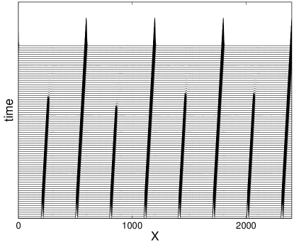
Figure 4: Space-time plot of the activator $u(x,t)$ demonstrating the spatially inhomogeneous pitchfork bifurcation. Equation parameters are $\epsilon=0.04897125$ and $L=300$; all other parameters are as in Figure 1. Initially there is an initial group of $8$ pulses which after some time exhibits a spatial period-doubling instability and subsequently evolves into a stable propagating wave train consisting of $4$ remaining pulses.

The above mentioned inhomogeneous alternating instability is contained in our normal form. To investigate spatial instabilities we need to distinguish between consecutive pulses. We may rewrite the normal form as

$$\partial_{t}X_{l}=-\mu-gX_{l}^{2}-\beta(\gamma+X_{l-1}(t-\tau)+\gamma_{1}X_{l}(t))\;,$$ (10)

where the subscript $l$ numbers the pulses in a wave train which interact with their nearest neighbours. Linearizing around the homogeneous solution $X_{l}={\bar{X}}$ according to

$$X_{l}={\bar{X}}+\delta e^{\sigma t}e^{ipl}\quad{\rm and}\quad X_{l-1}={\bar{X}}+\delta e^{\sigma t}e^{ip(l-1)}$$

yields as a condition for stationary instabilities (ie. $\sigma=0$)

$${\bar{X}}=-\frac{\beta}{2g}(\gamma_{1}+\cos{p}-i\sin{p})\;.$$

Hence stationary instabilities are possible for $p=0$ and for $p=\pi$. In the homogeneous case $p=0$, the instability is yet again the spatially homogeneous saddle-node (5). For $p=\pi$ this is a new type of instability, and we have ${\bar{X}}=\beta(1-\gamma_{1})/2g$ at the bifurcation point. This spatially inhomogeneous bifurcation will be identified further down as a subcritical pitchfork bifurcation. The criterion $p=\pi$ for the inhomogeneous bifurcation is corroborated by numerical simulations where every second pulse dies within a wave train (see Figure 4). Note that in traveling wave coordinates of a partial differential equation model for excitable media, this instability would correspond to a subcritical period-doubling bifurcation.

In order to study this $p=\pi$-bifurcation within our normal form we need to consider two populations of pulses ($l=1,2$), $X$ and $Y$, which interact via their inhibitors with each other. We extend our normal form for the case $p=\pi$ to

$$\partial_{t}X = -\mu-gX^{2}-\beta(\gamma+Y(t-\tau)+\gamma_{1}X(t))$$

$$\partial_{t}Y = -\mu-gY^{2}-\beta(\gamma+X(t-\tau)+\gamma_{1}Y(t))\;.$$ (11)

The system (4.4) for wave trains supports two types of stationary solutions; firstly the homogeneous solution (4), ${\bar{X}}_{h}={\bar{Y}}_{h}$, which may undergo a saddle-node bifurcation described by (5). There exists another stationary solution, an alternating mode, with

$${\bar{X}}_{a}=-{\bar{Y}}_{a}+\frac{\beta}{g}(1-\gamma_{1})\;.$$ (12)

Associated with this solution is a pitchfork bifurcation at

$$\mu_{PF}=\frac{1}{4}\frac{\beta^{2}(1+\gamma_{1})^{2}}{g}-\frac{\beta^{2}}{g}-\beta\gamma={\bar{\mu}}_{SN}-\frac{\beta^{2}}{g}\leq\mu_{SN}\;,$$ (13)

when

$$X_{PF}=Y_{PF}=\frac{\beta}{2g}(1-\gamma_{1})\;.$$ (14)

Comparing (5) with (13) shows that the pitchfork bifurcation sets in before the saddle-node bifurcation. The upper branch of the homogeneous solution ${\bar{X}}_{h}$ given by (4) at the pitchfork bifurcation point $\mu_{PF}$ coincides with (14). Hence the pitchfork bifurcation branches off the upper branch of the homogeneous solution. It is readily seen that the pitchfork bifurcation is subcritical because there are no solutions ${\bar{X}}_{a}$ possible for $\mu>\mu_{PF}$.

We now look at the stability of the homogeneous solution ${\bar{X}}={\bar{Y}}={\bar{X}}_{h}={\bar{Y}}_{h}$. We study perturbations $X={\bar{X}}_{h}+x\exp{\sigma t}$ and $Y={\bar{X}}_{h}+y\exp{\sigma t}$. Linearization yields as a condition for nontrivial solutions $x$ and $y$.

$$(\sigma+2g{\bar{X}}_{h}+\beta\gamma_{1})=\pm\beta e^{-\sigma\tau}\;.$$ (15)

The upper sign refers to an antisymmetric mode $x=-y$ whereas the lower sign refers to a symmetric mode $x=y$. Stationary bifurcations occur at $\sigma=0$. The symmetric mode then coincides with the saddle-node bifurcation (5) whereas the antisymmetric mode terminates at the pitchfork bifurcation (14).

Non-stationary Hopf bifurcations are possible if $\sigma=i\omega$. We then have

$$\omega=\mp\beta\sin{\omega\tau}$$ (16)

and

$${\bar{X}}_{h}=\frac{\beta}{2g}(\pm\cos{\omega\tau}-\gamma_{1})\;.$$ (17)

One has physical solutions with a single-valued positive $\omega$ only for the symmetric case (the lower signs) which reproduces our results (7) and (8) for the symmetry preserving Hopf bifurcation. For $\omega\tau\to 0$ the Hopf bifurcation moves towards the saddle-node (5) and coalesces with it at $\beta\tau=1$ in a Bogdanov-Takens point as described in Section 4. For $\omega\tau\to\pi$ the limiting value of ${\bar{X}}_{h}$ is ${\bar{X}}_{h}=\beta(1-\gamma_{1})/(2g)$ which coincides with the pitchfork bifurcation $X_{PF}$ in another codimension-2 bifurcation. At this bifurcation the Hopf bifurcation has a period $T=2\tau$ which corresponds exactly to the inhomogeneous pitchfork bifurcation with $p=\pi$ whereby every second pulse dies.

For values $\omega\tau\in[0,\pi)$ the Hopf bifurcation always comes after the pitchfork bifurcation which has been numerically verified with simulations of the full system (2).

Figure 5: Sketch of the bifurcation diagram for a wave train in a ring showing a stationary saddle-node bifurcation (SN) and a subcritical pitchfork bifurcation (PF).

This allows us to sketch the full bifurcation scenario for a wave train in a periodic ring as depicted in Figure 5.

5 Determination of the parameters of the normal form

In this Section we determine the parameters of the normal form (3) from numerical simulations of the full partial differential equations (2). We determine the free parameters $\nu$, $\mu$, $g$, $\gamma$, $\gamma_{1}$ and $\beta_{0}$. We are then in the position to test how well the normal form (3) reproduces the solution behaviour of the full partial differential equation (2). We use here as equation parameters for (2) $a=0.22$, $u_{s}=0.1$ and $D=1$.

The parameter $\nu$ which modifies the delay time $\tau$ due to the finite width of a pulse is easily determined as a typical width of a pulse in the parameter region of interest. We find $\nu=32$. We note that there is some ambiguity in the determination of $\nu$, and one may as easily justify $\nu\in[29,34]$.

The parameters $\mu$ and $g$ can be determined by studying the isolated pulse with $L\to\infty$. The normal form reduces to

$$\partial_{t}X=-\mu-gX^{2}\;.$$ (18)

We have $\mu=\alpha(\epsilon-\epsilon_{c})$ with $\epsilon_{c}$ being the critical $\epsilon$ at the saddle-node. Solutions of (18) are obtained by quadrature

$$X(t) = \sqrt{\frac{-\mu}{g}}\tanh(\sqrt{-\mu g}(t-t_{0}))\quad{\rm{for}}\quad\mu<0$$

$$\quad X(t) = -\sqrt{\frac{\mu}{g}}\tan(\sqrt{\mu g}(t-t_{0}))\quad\,\,\,\quad{\rm{for}}\quad\mu>0\;.$$ (19)

For small deviations from the saddle-node $X=0$ this solution may be expanded to obtain $X(t)\approx\mu t$ which obviously corresponds to the solution of equation (18) linearized around the saddle-node. The solution (5) has its inflection point at the saddle-node $X=0$ where its slope is $\mu$. We can therefore determine $\mu$ by measuring $\partial_{t}X$ at the inflection point for different values of $(\epsilon-\epsilon_{c})$. This allows us to determine $\alpha$ via $\alpha=\mu/(\epsilon-\epsilon_{c})$. In Figure 6 we show the results of $\partial_{t}X$ versus $(\epsilon-\epsilon_{c})$. The numerical results are obtained by letting a stable pulse which was created at some $\epsilon<\epsilon_{c}$, decay in an environment with $\epsilon>\epsilon_{c}$. The relaxation then allows us to determine the slope at the saddle-node. Using a least-square fit we obtain $\alpha=1.455$.

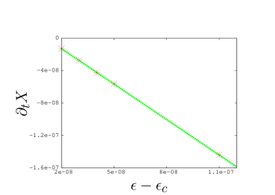
Figure 6: The temporal derivative $\partial_{t}X$ at the saddle-node versus $\epsilon-\epsilon_{c}$. The slope determines the parameter $\alpha=\mu/(\epsilon-\epsilon_{c})$. The stars are obtained by numerically integrating the partial differential equation (2). The line is a least-square fit.

The parameter $g$ can now be determined by looking at the stationary problem $\partial_{t}X=0$. The behaviour of the amplitude of the activator close to the saddle-node versus $\epsilon$ is depicted in Figure 7. It clearly demonstrates quadratic behaviour typical for saddle-nodes. The normal form for the saddle-node of an isolated pulse (2) yields $(\epsilon-\epsilon_{c})=(g/\alpha)X^{2}$ which we can use upon using the above measured value of $\alpha$ to obtain $g=0.31$ from a least square fit.

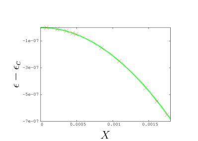
Figure 7: Bifurcation parameter $\epsilon-\epsilon_{c}$ versus amplitude $X$ close to the saddle-node of the isolated pulse. The crosses are obtained by numerically integrating the partial differential equation (2). The line is a quadratic fit.

To determine the missing parameters $\beta_{0}$, $\gamma$ and $\gamma_{1}$ we need to study a pulse in a periodic ring of finite length $L$. The self-interaction of the pulse with its own inhibitor modifies the saddle-node bifurcation as discussed in Section 3. We will look here at the symmetry preserving Hopf bifurcation. To study the Hopf bifurcation we study the circulation of a single pulse in a periodic ring instead of a wave train consisting of more than one pulse. In the latter case the subcritical pitchfork bifurcation sets in before the symmetry preserving Hopf bifurcation.

Combining the expressions for the angular frequency $\omega$ and the deviation ${\bar{X}}_{HH}$ of the pulse amplitude from the saddle-node at the bifurcation point, (7) and (8), we can eliminate the so far undetermined parameter $\beta$ to determine $\gamma_{1}$. We obtain

$$\frac{{\bar{X}}_{HH}}{\omega}=-\frac{1}{2g}(\cot(\omega\tau)+\gamma_{1}\sin^{-1}(\omega\tau))\;.$$ (20)

In Figure 8 we show a plot of numerically obtained values for the quantity ${\bar{X}}_{HH}/\omega$ by integrating the partial differential equation (2), and the result of our normal form (20). In the numerical simulations of (2) we measured the frequency of the subcritical Hopf bifurcation $\omega$ and ${\bar{X}}_{HH}$ which is the difference between the amplitude at the symmetry preserving Hopf bifurcation and the saddle-node value of the isolated pulse. Expression (20) matches the numerical simulations well for $\gamma_{1}=0.31$.

Figure 8: Plot of ${\bar{X}}_{HH}/\omega$ versus $\omega\tau$. The crosses depict results from numerically integrating the full partial differential equation (2). The line represents the analytical expression (20) of our normal form. This fit is achieved by choosing $\gamma_{1}=0.31$.

We can now determine the parameters $\beta_{0}$ and $\gamma$ by looking at the shift of the bifurcation parameter $\mu$ and the shift of the critical amplitude $X$ at the saddle-node for finite wavelength $L$ with respect to the values at the saddle-node for an isolated pulse with infinite wavelength. The saddle-node is shifted with respect to the isolated pulse with $\mu_{SN}=X_{SN}=0$. We express the shifted finite-$L$ saddle-node by

$$\mu+\delta=-g(X-\xi)^{2}\;,$$

where $\delta=\delta(L)$ expresses the shift in the bifurcation parameter at the saddle-node and $\xi=\xi(L)$ expresses the shifted value of the amplitude when compared to the isolated pulse.

The values for $\delta(L)$ and $\xi(L)$ can be measured by numerically solving (2) and determing the finite wavelength induced saddle-node. We did so by expressing (2) in travelling wave coordinates and treating the problem as a boundary value problem. The thereby obtained values for $\delta(L)$ and $\xi(L)$ have to be compared with the corresponding expressions of the normal form. In the normal form (3) the finite wavelength induced shift is represented by the finite length correction

$$V(t-\tau)=\beta_{0}\exp(-a\epsilon(L-\nu)/c)\left(\gamma+X(t-\tau)+\gamma_{1}X(t)\right)\;.$$

Neglecting ${\cal{O}}(\xi^{2})$ which is justified for not too large deviations from the isolated pulse, we obtain

$$\delta = \gamma\beta_{0}\;\exp(-\epsilon a(L-\nu)/c)$$ (21)

$$\xi = \frac{\beta_{0}}{2g}(1+\gamma_{1})\;\exp(-\epsilon a(L-\nu)/c)\;,$$ (22)

where $\nu$ and $\gamma_{1}$ had already been determined. Note that the ${\cal{O}}(\xi^{2})$-term, $g\xi^{2}=\beta^{2}(1+\gamma_{1})/4g$ appears, of course, correctly in the shift of the bifurcation parameter $\mu_{SN}$ in (5). Although the inclusion of $\gamma_{1}\neq 0$ is not necessary for the existence of a Hopf bifurcation (see (7,8)), it is significant to obtain good quantitative agreement. Whereas for the stationary bifurcations the inclusion of $\gamma_{1}$ is in effect a redefinition of $\beta$, it is vital in the case of the Hopf bifurcation because it allows for a decoupled dependence of the frequency $\omega$ and the amplitude ${\bar{X}}_{HH}$ on $L$. In Figure 9 we show a plot of the bifurcation parameter shift as a function of length $L$. Agreement of numerically obtained values from a simulation of the full partial differential equation (2) with the expression derived from our normal form (21), which implies $\delta=\alpha(\epsilon-\epsilon_{c})$ is assured provided $\gamma\beta_{0}=0.115$. We recall that $\epsilon_{c}$ is the critical refractoriness at the saddle-node of an isolated pulse. In Figure 10 we show a plot of the pulse amplitude shift as a function of length $L$. Agreement of numerically obtained values from a simulation of the full partial differential equation (2) with the expression derived from our normal form (22) is given provided $(\beta_{0}/2g)(1+\gamma_{1})=1.1$. Combining these results we can solve for $\beta_{0}$ and $\gamma$ and obtain $\gamma=0.32$ and $\beta_{0}=0.53$. This finalizes the determination of the free parameters of the normal form (3).

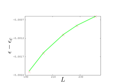
Figure 9: Shift of the bifurcation parameter $(\epsilon-\epsilon_{c})$ at the saddle-node as a function of $L$. Crosses depict results from a numerical simulation of the full partial differential equation (2). The line represent the analytical expression (21) of our normal form. Agreement of the two curves is achieved for $\gamma\beta_{0}=0.115$.

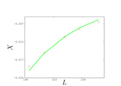
Figure 10: Shift of the amplitude deviation $X$ at the saddle-node as a function of $L$. Crosses depict results from a numerical simulation of the full partial differential equation (2). The line represent the analytical expression (22) of our normal form. Agreement of the two curves is achieved for $(\beta_{0}/2g)(1+\gamma_{1})=0.91$.

We are now in the position to check the validity of our normal form by testing whether the normal form (3) with the above determined parameters is able to reproduce observations of the numerical simulation of the full partial differential equation (2). We already noted in Section 4 qualitative agreement i.e. the correct bifurcation behaviour. Here we show quantitative agreement with the behaviour of (2).
In particular we look at the symmetry preserving Hopf bifurcation described in Section 4. In Figure 11 and Figure 12 we show a comparison of the analytical results for the frequency and the amplitude at the Hopf bifurcation, (7) and (8), with results obtained from numerically integrating (2). The Figures show good agreement. Note that the parameters $\beta_{0}$ and $\nu$ were not determined by fitting data representing the symmetry preserving Hopf bifurcation and henceforth the two figures, Figure 11 and Figure 12, are indeed predictions.

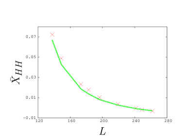
Figure 11: Amplitude deviation at the Hopf bifurcation ${\bar{X}}_{HH}$ as a function of $L$. Crosses depict results from a numerical simulation of the full partial differential equation (2). The line represent the analytical expression (8) of our normal form.

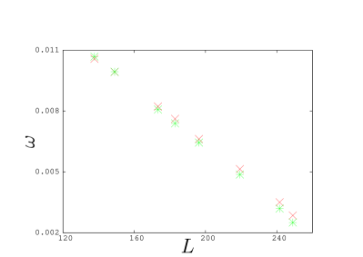
Figure 12: Angular frequency at the Hopf bifurcation $\omega$ as a function of $L$. Crosses depict results from a numerical simulation of the full partial differential equation (2). Stars were obtained by solving the analytical expression (7) of our normal form for $\omega$.

Figure 13 shows a comparison of numerical simulations of (2) and our analytical results (14) for the spatially inhomogeneous pitchfork bifurcation. For the determination of the parameters of the normal form we have not used any fitting which involved results from the spatially inhomogeneous pitchfork bifurcation. The agreement in Figure 13 therefore demonstrates that the normal form can indeed be used to obtain quantitative agreement and make quantitative predictions.

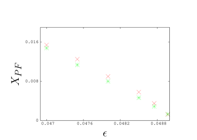
Figure 13: Amplitude deviations at the pitchfork bifurcation ${\bar{X}}_{PF}$ as a function of $\epsilon$. Crosses depict numerical results from integrating the full partial differential equation (2). Stars show the corresponding values calculated by using the normal form result (14).

6 Summary and discussion

We have constructed a normal form for travelling waves in one-dimensional excitable media which takes the form of a delay differential equation. The construction is based on the well-known observation that the interaction of a pulse with the inhibitor of the preceding pulse modifies the generic saddle-node bifurcation of an isolated pulse. The normal form (3) exhibits a rich bifurcation behaviour which we could verify by numerically simulating the partial differential equation (2). Besides the well known saddle-node bifurcations for isolated pulses and for periodic wave trains the normal form also exhibits a symmetry preserving Hopf bifurcation and a symmetry breaking, spatially inhomogeneous pitchfork bifurcation. Moreover, the normal form shows that the saddle-node and the Hopf bifurcation are an unfolding of a Bogdanov-Takens point as previously suggested in [27, 23]. The symmetry preserving Hopf bifurcation is found to occur before the saddle-node bifurcation for a single pulse in a ring. For a wave train consisting of several pulses in a ring, the Hopf- and the saddle-node bifurcations occur after the symmetry breaking pitchfork bifurcation in which every second pulse dies. We could verify these scenarios in numerical simulations of the modified Barkley-model (2) and the Fitzhugh-Nagumo equations [26]. These bifurcations have been observed before but had previously not been described within a unified framework of one normal form.
We were able to determine the parameters of the normal form from numerical simulations of the partial differential equation (2). Using these numerically determined parameters we showed excellent agreement between the normal form and the full partial differential equation (2). We could quantitatively describe the symmetry preserving Hopf bifurcation and the inhomogeneous pitchfork bifurcation. Moreover, we were able to quantify the Bogdanov-Takens bifurcation.

The symmetry preserving Hopf bifurcation has been studied intensively before. It was observed numerically for example for the Barkley-model [27]. Interest has risen in the Hopf bifurcation in the context of cardiac dynamics because it leads to propagation failure of a single pulse on a ring. It is believed to be related to a phenomenon in cardiac excitable media which goes under the name of alternans. Alternans describe the scenario whereby action potential durations are alternating periodically between short and long periods. The interest in alternans has risen as they are believed to trigger spiral wave breakup in cardiac tissue and ventricular fibrillation [12, 11, 32, 13, 38]. Besides numerical investigations of the Barkley model [27], the modified Barkley model [23], the Beeler-Reuter model [28, 11, 29, 30], the Noble-model [32, 29] and the Karma-model [32], where a Hopf bifurcation has been reported, there have been many theoretical attempts to quantify this bifurcation for a single-pulse on a ring. Since the pioneering work [12] alternans have been related to a period-doubling bifurcation. It was proposed that the bifurcation can be described by a one-dimensional return map relating the action potential duration ($APD$) to the previous recovery time, or diastolic interval ($DI$), which is the time between the end of a pulse to the next excitation. A period-doubling bifurcation was found if the slope of the so called restitution curve which relates the $APD$ to the $DI$, exceeds one. A critical account on the predictive nature of the restitution curve for period-doubling bifurcations is given in [39, 36]. In [29] the instability was analyzed by reducing the partial differential equation describing the excitable media to a discrete map via a reduction to a free-boundary problem. In [23] the Hopf bifurcation could be described by means of a reduced set of ordinary-differential equations using a collective coordinate approach. In [11, 30] the bifurcation was linked to an instability of a single integro-delay equation. The condition for instability given by this approach states - as in some previous studies involving one-dimensional return maps - that the slope of the restitution curve needs to be greater than one. However, as evidenced in experiments [40] and in theoretical studies [39, 36] alternans do not necessarily occur when the slope of the restitution curve is greater than one. In further studies it would be interesting to see how our criterion $\beta\tau\geq 1$ is related to that condition. Note that $\nu$ is related to the $APD$ and $\tau=(L-\nu)/c$ to the recovery time $DI$.
In the context of alternans the Hopf bifurcation has been described as a supercritical bifurcation [11, 32, 29, 30] (although their occurrence is related to wave break up [29]). Further study will explore whether the subcritical character of the Hopf bifurcation we find is model-dependant or indeed generic.

To go beyond the case of a single pulse circulating in a ring, periodically stimulated excitable media have been studied in the context of alternans [41, 42, 35, 34, 36, 37]. In [41, 36] one-dimensional maps were developed to study the Hopf bifurcation and the transition to conduction blocks. In [35] a nonlocal partial differential equation has been proposed to study spatiotemporal dynamics of alternans. It would be interesting for further studies to see how the transition to conduction blocks explored in these paced cardiac excitable media [34, 35, 36, 37] can be described by the spatially inhomogeneous pitchfork bifurcation we found in our normal form. The pitchfork bifurcation however does not require a fixed pacing site and does not require external pacing but rather is dynamically induced. This may aid in investigating the formation of conduction blocks purely as a dynamical phenomenon of wave trains.
An interesting scenario in our normal is the coalescence of the spatially inhomogeneous pitchfork bifurcation with the Hopf bifurcation when $\omega\tau=\pi$. This condition implies $T=2\tau$. Then the Hopf frequency is in resonance with the spatial instability in which every second pulse dies. Connections to alternans of this scenario are planned for further research.

Ideally, one would like to deduce the normal form directly from a model for excitable media and determine its parameters without relying on numerical simulations of a particular excitable medium. One initial path along that avenue could be to use the non-perturbative approach developed in [23] to determine the parameters. This method was developed to study critical wave propagation of single pulses and pulse trains in excitable media in one and two dimensions. It was based on the observation that close to the bifurcation point the pulse shape is approximately a bell-shaped function. Numerical simulations show that this is the case for the Barkley model (2) close to the saddle-node bifurcation. A test function approximation that optimises the two free parameters of a bell-shaped function, i.e. its amplitude and its width, allows us to find the actual bifurcation point, $\epsilon_{c}$, and determine the pulse shape for close-to-critical pulses at excitabilities near $\epsilon_{c}$. This method has so far also been successfully applied to other non-excitable reaction-diffusion equations [43, 44]. To apply the method for our purpose is planned for future work.

Acknowledgements G.A.G gratefully acknowledges support by the Australian Research Council, DP0452147. G.A.G. would like to thank Björn Sandstede for kindly helping with producing some of the numerical saddle-node values using AUTO. Initial parts of the simulations were done with the XDim Interactive Simulation Package developed by P. Coullet and M. Monticelli.

References

- [1] A.T. Winfree, When Time Breaks Down (Princeton University Press, 1987).
- [2] J.M. Davidenko, A.M. Pertsov, R. Salomonsz, W. Baxter and J. Jalife, Nature 335, 349 (1992).
- [3] F. Siegert and C. Weijer, Physica 49D, 224 (1991).
- [4] M. Berridge, P. Lipp and M. Bootman, NatureReviews Molecular Cell Biology 1, 11 (2000).
- [5] A. T. Winfree, Science 266, 175 (1972).
- [6] A. T. Winfree, SIAM. Rev. 32, 1 (1990).
- [7] A. T. Winfree, Science 266, 1003 (1994).
- [8] D. Margerit and D. Barkley, Phys. Rev. Lett. 86, 175 (2001).
- [9] D. Margerit and D. Barkley, Chaos 12, 636 (2002).
- [10] see review articles in the focus issue Chaos 8, 1 (1998).
- [11] M. Courtemanche, L. Glass and J. Keener, Phys. Rev. Lett. 70, 2182 (1993).
- [12] J.B. Nolasco and R.W. Dahlen, J. Appl. Physiol. 25, 191 (1968).
- [13] A. Karma, Chaos 4, 461 (1994).
- [14] A. S. Mikhailov, Foundations of Synergetics I: distributed Active Systems, 2nd edition, Springer Verlag, Berlin (1994).
- [15] W. Jahnke and A.T. Winfree, Int. J. Bifurcation. Chaos 1, 445 (1991).
- [16] V.S. Zykov, Simulation of Wave Processes in Excitable Media, (Manchester Univ. Press, New York, 1987).
- [17] A.S. Mikhailov, V.A. Davydov and V.S. Zykov, Physica 70D, 1 (1994).
- [18] E. Meron, Physics Report 218, (1992).
- [19] V. Hakim and A. Karma, Phys. Rev. Lett. 79, 665 (1997).
- [20] V. Hakim and A. Karma, Phys. Rev. E 60, 5073 (1999).
- [21] D. Barkley and I.G. Kevrekidis, Chaos 4, 453 (1994).
- [22] P. Ashwin, I. Melbourne and M. Nicol, Nonlinearity 12, 741 (1999).
- [23] G. Gottwald and L. Kramer, Chaos 14, 855 (2004).
- [24] D. Barkley, Physica 49D, 61 (1991).
- [25] J. Keener and J. Sneyd, Mathematical Physiology, Springer Verlag, New-York (1998).
- [26] R. Fitzhugh, Biophys. J. 1, 445 (1961); J. Nagumo, S. Arimoto and S. Yoshizawa, Proc. IRE 50, 2061 (1962).
- [27] M. Knees, L. S. Tuckerman and D. Barkley, Phys. Rev. A 46, 5054 (1992).
- [28] W. Quan and Y. Rudy, Circ. Res. 66, 367 (1990).
- [29] A. Karma, H. Levine and X. Zou, Physica D 73, 113 (1994).
- [30] M. Courtemanche, L. Glass and J. Keener, SIAM J. Appl. Math. 56, 119 (1996).
- [31] G. W. Beeler and H. Reuter, J. Physiol. 268, 177 (1977)
- [32] A. Karma, Phys. Rev. Lett. 71, 1103 (1993).
- [33] D. Noble, J. Physiol. 160, 317 (1962)
- [34] H. M. Hastings, F. H. Fenton, S. J. Evans, O. Hotomaroglu, J. Geetha, K. Gittelson, J. Nilson and A. Garfinkel. Phys. Rev. E 62, 4043 (2000).
- [35] B. Echebarria and A. Karma, Phys. Rev. Lett. 88, 208101 (2002).
- [36] J. J. Fox, E. Bodenschatz and R. F. Gilmour, Phys. Rev. Lett. 89, 138101 (2002).
- [37] H. Henry and W. -J. Rappel, Phys. Rev. E 71 , 051911 (2005).
- [38] F. H. Fenton, E. M. Cherry, H. M. Hastings and S. J. Evans, Chaos 12, 852 (2002).
- [39] F. H. Fenton, S. J. Evans and H. M. Hastings, Phys. Rev. Lett. 83, 3964 (1999).
- [40] G. M. Hall, S. Bahar and D. J. Gauthier, Phys. Rev. Lett. 82, 2995 (1999).
- [41] M. R. Guevara, L. Glass and A. Shrier, Science 214, 1350 (1981).
- [42] T. J. Lewis and M. R. Guevara, J. Theor. Biol. 146, 407 (1990).
- [43] S. Menon and G. A. Gottwald, Phys. Rev. E 71, 066201 (2005).
- [44] S. Cox and G. A. Gottwald, submitted to Physica D.