Influence of helicity on anomalous scaling of a passive scalar advected by the turbulent velocity field with finite correlation time:
Two-loop approximation

Abstract

The influence of helicity on the stability of scaling regimes, on the effective diffusivity, and on the anomalous scaling of structure functions of a passive scalar advected by a Gaussian solenoidal velocity field with finite correlation time is investigated by the field theoretic renormalization group and operator product expansion within the two-loop approximation. The influence of helicity on the scaling regimes is discussed and shown in the plane of exponents $\varepsilon-\eta$, where $\varepsilon$ characterizes the energy spectrum of the velocity field in the inertial range $E\propto k^{1-2\varepsilon}$, and $\eta$ is related to the correlation time at the wave number $k$, which is scaled as $k^{-2+\eta}$. The restrictions given by nonzero helicity on the regions with stable fixed points that correspond to the scaling regimes are analyzed in detail. The dependence of the effective diffusivity on the helicity parameter is discussed. The anomalous exponents of the structure functions of the passive scalar field which define their anomalous scaling are calculated and it is shown that, although the separate composite operators which define them strongly depend on the helicity parameter, the resulting two-loop contributions to the critical dimensions of the structure functions are independent of helicity. Details of calculations are shown.

I Introduction

During the last decade much attention has been paid to the inertial range of fully developed turbulence, which contains wave numbers larger than those that pump the energy into the system and smaller than those that are related to the dissipation processes MonYagBook ; HuPhWi91 . Grounding for the inertial range turbulence was created in the well known Kolmogorov–Obukhov (KO) phenomenological theory (see, e.g., MonYagBook ; McComb ; Frisch ). One of the main problems in the modern theory of fully developed turbulence is to verify the validity of the basic principles of KO theory and their consequences within the framework of a microscopic model. Recent experimental and theoretical studies indicate possible deviations from the celebrated Kolmogorov scaling exponents. The scaling behavior of velocity fluctuations with exponents whose values are different from Kolmogorov ones is called anomalous and usually is associated with the intermittency phenomenon. In turbulence this phenomenon is believed to be related to strong fluctuations of the energy flux which therefore leads to the deviations from the predictions of the aforementioned KO theory. Such deviations, referred to as anomalous or nondimensional scaling, manifest themselves in a singular dependence of the correlation or structure functions on the distances and the integral (external) turbulence scale $L$. The corresponding exponents are certain nontrivial and nonlinear functions of the order of the correlation function, the phenomenon referred to as “multiscaling.” Even though great progress in the understanding of intermittency and anomalous scaling in turbulence was achieved as a result of intensive studies, their investigation in fully developed turbulence still remains a major theoretical problem.

Although the theoretical description of fluid turbulence on the basis of first principles, i.e., on the stochastic Navier-Stokes equation MonYagBook , remains essentially an open problem, considerable progress has been achieved in understanding simplified model systems that share some important properties with the real problem: shell models Dyn , the stochastic Burgers equation Burgulence , and passive advection by random “synthetic” velocity fields FaGaVe01 .

A crucial role in these studies is played by models of the advected passive scalar field Obu49 . A simple model of a passive scalar quantity advected by a random Gaussian velocity field, white in time and self-similar in space (the latter property mimics some features of a real turbulent velocity ensemble), the so-called Kraichnan rapid-change model Kra68 , is an example. The interest in these models is based on two important facts: first, as shown by both natural and numerical experimental investigations, the deviations from the predictions of the classical Kolmogorov-Obukhov phenomenological theory MonYagBook ; OrszagBook ; Frisch ; McComb are even more strongly displayed for a passively advected scalar field than for the velocity field itself (see, e.g., AnHoGaAn84 ; Sre91 ; HolSig94 ; Pumir94 ; TonWar94 ; ElKlRo90te and references cited therein), and second, the problem of passive advection is much easier to consider from a theoretical point of view. In these studies the anomalous scaling was established on the basis of a microscopic model Kraichnan94 , and corresponding anomalous exponents were calculated within controlled approximations all ; Shraiman ; Pumir (see also the review FaGaVe01 and references therein).

The greatest stimulation to study the simple models of passive advection not only of scalar fields but also of vector fields (e.g., a weak magnetic field) is related to the fact that even simplified models with given Gaussian statistics of a so-called synthetic velocity field describes a lot of features of the anomalous behavior of genuine turbulent transport of some quantities (such as heat or mass) observed in experiments (see, e.g., Refs. Kra68 ; HolSig94 ; Pumir94 ; TonWar94 ; ElKlRo90te ; all ; Shraiman ; Pumir ; AveMaj90 ; ZhaGli92 ; Kraichnan94 ; KrYaCh95 and references cited therein).

An effective method for investigation of a self-similar scaling behavior is the renormalization group (RG) technique ZinnJustin ; Vasiliev ; Collins . It was widely used in the theory of critical phenomena to explain the origin of the critical scaling and also to calculate corresponding universal quantities (e.g., critical dimensions). This method can also be directly used in the theory of turbulence Vasiliev ; deDoMa79 ; AdVaPi83 ; AdAnVa96 ; AdAnVa99 , as well as in related models like the simpler stochastic problem of a passive scalar advected by a prescribed stochastic flow. In what follows we use the conventional (”quantum field theory” or field theoretic) RG which is based on the standard renormalization procedure, i.e., on elimination of the ultraviolet (uv) divergences.

In Refs. AdAnVa98+ the field theoretic RG and operator-product expansion (OPE) were used in the systematic investigation of the rapid-change model. It was shown that within the field theoretic approach the anomalous scaling is related to the very existence of so-called dangerous composite operators with negative critical dimensions in the OPE (see, e.g., Vasiliev ; AdAnVa99 for details). In subsequent papers AdAnBaKaVa01 the anomalous exponents of the model were calculated within the $\varepsilon$ expansion to order $\varepsilon^{3}$ (three-loop approximation). Here $\varepsilon$ is a parameter that describes a given equal-time pair correlation function of the velocity field (see later section). Important advantages of the RG approach are its universality and calculational efficiency: a regular systematic perturbation expansion for the anomalous exponents was constructed, similar to the well-known $\epsilon$ expansion in the theory of phase transitions.

Afterward, various generalized descendants of the Kraichnan model, namely, models with inclusion of large and small scale anisotropy AdAnHnNo00 , compressibility AdAn98 , and finite correlation time of the velocity field Antonov99 ; Antonov00 were studied by the field theoretic approach. Moreover, advection of a passive vector field by the Gaussian self-similar velocity field (with and without large and small scale anisotropy, pressure, compressibility, and finite correlation time) has also been investigated and all possible asymptotic scaling regimes and crossovers among them have been classified all1 . The general conclusion is that the anomalous scaling, which is the most important feature of the Kraichnan rapid-change model, remains valid for all generalized models.

Let us describe briefly the solution of the problem in the framework of the field theoretic approach (see, e.g., Refs. Vasiliev ; AdAnVa96 ; AdAnVa99 for more details). It can be divided into two main stages. In the first stage the multiplicative renormalizability of the corresponding field theoretic model is demonstrated and the differential RG equations for its correlation functions are obtained. The asymptotic behavior of the latter on their ultraviolet argument $(r/\ell)$ for $r\gg\ell$ and any fixed $(r/L)$ is given by infrared stable fixed points of those equations. Here $\ell$ and $L$ are the inner (ultraviolet) and the outer (infrared) scales. The behavior involves some “scaling functions” of the infrared argument $(r/L)$, whose form is not determined by the RG equations. In the second stage, their behavior at $r\ll L$ is found from the OPE within the framework of the general solution of the RG equations. There, the crucial role is played by the critical dimensions of various composite operators, which give rise to an infinite family of independent scaling exponents as mentioned above (and hence to multiscaling). Of course, both these stages (and thus the phenomenon of multiscaling) have long been known in the RG theory of critical behavior. The distinguishing feature specific to models of turbulence is the existence of composite operators with the aforementioned negative critical dimensions. Their contributions to the OPE diverge at $(r/L)\to 0$. In models of critical phenomena, nontrivial composite operators always have strictly positive dimensions, so that they only determine corrections [vanishing for $(r/L)\to 0$] to the leading terms [finite for $(r/L)\to 0$] in the scaling functions.

In Ref. Antonov99 the problem of a passive scalar advected by a Gaussian self-similar velocity field with finite correlation time all2 was studied by the field theoretic RG method. There, a systematic study of the possible scaling regimes and anomalous behavior was presented at one-loop level. The two-loop corrections to the anomalous exponents were obtained in Ref. AdAnHo02 . It was shown that the anomalous exponents are nonuniversal as a result of their dependence on a dimensionless parameter, the ratio of the velocity correlation time and the turnover time of the scalar field.

In what follows, we shall continue with the investigation of this model from the point of view of the influence of helicity (spatial parity violation) on the scaling regimes and anomalous exponents within the two-loop approximation.

Helicity is defined as the scalar product of velocity and vorticity and its nonzero value expresses mirror symmetry breaking of the turbulent flow. It plays a significant role in the processes of magnetic field generation in an electrically conductive fluid dynamo1 -Steh3 and represents one of the most important characteristics of large-scale motions as well Etling85 -Ponomar2003 . The presence of helicity is observed in various natural (like large air vortices in the atmosphere) and technical flows Moffat92 ; Kholmyansky2001 ; Koprov2005 . Despite this fact the role of the helicity in hydrodynamical turbulence is not completely clarified up to now.

The Navier-Stokes equations conserve kinetic energy and helicity in the inviscid limit. The presence of two quadratic invariants leads to the possibility of appearance of double cascade. This means that cascades of energy and helicity take place in different ranges of wave numbers analogously to the two-dimensional turbulence and/or the helicity cascade appearing concurrently to the energy cascade in the direction of small scales Brissaud73 ; Moiseev1996 . In particular, the helicity cascade is closely connected with the existence of the exact relation between triple and double correlations of velocity known as the 2/15 law analogously to the 4/5 Kolmogorov law Chkhet96 . Corresponding to Brissaud73 the aforementioned scenarios of turbulent cascades differ from each other by spectral scaling. Theoretical arguments given by Kraichnan Kraich73 and results of numerical calculations of the Navier-Stokes equations Andre77 ; Orszag1997 ; Chen2003 support the scenario of concurrent cascades. The appearance of helicity in turbulent systems leads to the constraint of the nonlinear cascade to small scales. This phenomenon was first demonstrated by Kraichnan Kraich73 within the modeling problem of statistically equilibrium spectra and later in numerical experiments.

Turbulent viscosity and diffusivity, which characterize the influence of small-scale motions on heat and momentum transport, are basic quantities investigated in the theoretic and applied models. The constraint of the direct energy cascade in helical turbulence has to be accompanied by a decrease of turbulent viscosity. However, no influence of helicity on turbulent viscosity was found in some works Pouquet78 ; Zhou91 . A similar situation is observed for the turbulent diffusivity in helical turbulence. Although the modeling calculations demonstrate intensification of turbulent transfer in the presence of helicity Kraich761 ; Drum84 direct calculation of the diffusivity does not confirm this effect Kraich761 ; Knobl77 ; Lipscombe91 . Helicity is a pseudoscalar quantity, hence, it can be easily understood that its influence appears only in quadratic and higher terms of perturbation theory or in combination with other pseudoscalar quantities (e.g., large-scale helicity). Really, simultaneous consideration of memory effects and second order approximation indicates the effective influence of helicity on turbulent viscosity Belian1994 ; Belian1998 and turbulent diffusivity Drum84 ; Dolg87 ; Drummond2001 ; Chkhetiani2004 already in the limits of small and infinite correlation time.

Helicity, as we shall see below, does not affect known results in the one-loop approximation and, therefore, it is necessary to turn to the second order (two-loop) approximation to be able to analyze possible consequences. It is also important to say that in the framework of the classical Kraichnan model, i.e., a model of passive advection by a Gaussian velocity field with $\delta$-like correlations in time, it is not possible to study the influence of the helicity because all potentially helical diagrams are identically equal to zero at all orders in the perturbation theory. In this sense, the investigation of the helicity in the present model can be consider as the first step toward analyzing the helicity in genuine turbulence. In fact, it is interesting and important to study the helicity effects because many turbulence phenomena are directly influenced by them (like large air vortices in the atmosphere). For example, in stochastic magnetic hydrodynamics, which studies the turbulence in electrically conducting fluids, it leads to the nontrivial fact of the existence of a so-called turbulent dynamo – the generation of a large-scale magnetic field by the energy of the turbulent motion dynamo1 ; Moffatt ; AdVaHn87 ; HnJuSt01 ; Steh1 ; Steh2 ; Steh3 . This is an important effect in astrophysics.

The main result of the paper will be the conclusion that helicity does not change the anomalous exponents of the single-time structure functions within the two-loop approximation although the separate composite operators which define them strongly depend on the helicity parameter. This result leads to the following interesting but nontrivial question: is this result related only to the two-loop calculations or does it hold for all orders of perturbation theory? Of course, the answer to this question definitely lies at least within the three-loop approximation. On the other hand, as will be shown, the effective diffusivity rather strongly depends on the helicity parameter.

The paper is organized as follows. In Sec. II we present the definition of the model and introduce the helicity to the transverse projector of a given pair correlation function of the velocity field. In Sec. III we give the field theoretic formulation of the original stochastic problem and discuss the corresponding diagrammatic technique. In Sec. IV we analyze the ultraviolet divergences of the model, establish its multiplicative renormalizability, and calculate the renormalization constants in the two-loop approximation. In Sec. V we analyze possible scaling regimes of the model, associated with nontrivial and physically acceptable fixed points of the corresponding RG equations. There are five such regimes, any one of which can be realized in dependence on the values of the parameters of the model. We discuss the physical meaning of these regimes (e.g., some of them correspond to zero, finite, or infinite correlation time of the advecting field) and their regions of stability in the space of the model parameters. In Sec. VI the two-loop corrections to the effective diffusivity are calculated. In Sec. VII the renormalization of needed composite operators is done and their explicit dependence on the helicity parameter is shown. In Sec. VIII discussion of the results is present.

II The model

In what follows, we shall consider the advection of a passive scalar field $\theta\equiv\theta(x)\equiv\theta(t,{\bf x})$ which is described by the following stochastic equation:

$$\partial_{t}\theta+v_{i}\partial_{i}\theta=\nu_{0}\Delta\theta+f^{\theta},$$ (1)

where $\partial_{t}\equiv\partial/\partial t$, $\partial_{i}\equiv\partial/\partial x_{i}$, $\nu_{0}$ is the coefficient of molecular diffusivity (hereafter all parameters with a subscript $0$ denote bare parameters of the unrenormalized theory; see below), $\Delta\equiv\partial^{2}$ is the Laplace operator, $v_{i}\equiv v_{i}(x)$ is the $i$th component of the divergence-free (owing to the incompressibility) velocity field ${\bf v}(x)$, and $f^{\theta}\equiv f^{\theta}(x)$ is a Gaussian random noise with zero mean and correlation function

$$\langle f^{\theta}(x)f^{\theta}(x^{\prime})\rangle=\delta(t-t^{\prime})C({\bf r}/\tilde{L}),\,\,\,{\bf r}={\bf x}-{\bf x^{\prime}},$$ (2)

where the angular brackets $\langle...\rangle$ hereafter denote the average over the corresponding statistical ensemble. The noise maintains the steady state of the system but the concrete form of the correlator is not essential. The only condition that must be satisfied by the function $C({\bf r}/\tilde{L})$ is that it must decrease rapidly for $r\equiv|{\bf r}|\gg\tilde{L}$, where $\tilde{L}$ denotes an integral scale related to the stirring. In the case when $C$ depends not only on the modulus of the vector ${\bf r}$ but also on its direction, it plays the role of a source of large-scale anisotropy, whereupon the noise can be replaced by a constant gradient of scalar field. Equation (1) then reads (see, e.g., Ref. Antonov99 )

$$\partial_{t}\theta+v_{i}\partial_{i}\theta=\nu_{0}\Delta\theta-{\bf h}\cdot{\bf v}.$$ (3)

Here, $\theta(x)$ is the fluctuation part of the total scalar field $\Theta(x)=\theta(x)+{\bf h}\cdot{\bf x}$, and ${\bf h}$ is a constant vector that determines the distinguished direction. The direct formulation with a scalar gradient is even more realistic; see, e.g. Refs. HolSig94 ; Shraiman ; Pumir ; Antonov99 ; Antonov00 .

In real problems the velocity field ${\bf v}(x)$ satisfies the stochastic Navier-Stokes equation. In spite of this fact, in what follows, we shall suppose that the velocity field is driven by the simple linear stochastic equation HolSig94 ; Antonov99

$$\partial_{t}v_{i}+Rv_{i}=f^{v}_{i},$$ (4)

where $R\equiv R(x)$ is a linear operation to be specified below and $f^{v}_{i}\equiv f^{v}_{i}(x)$ is an external random stirring force with zero mean and the correlator

$$\langle f^{v}_{i}(x)f^{v}_{j}(x^{\prime})\rangle \equiv D^{f}_{ij}(x;x^{\prime})$$ (5)

$$= \int\frac{d\omega d^{d}k}{(2\pi)^{d+1}}P^{\rho}_{ij}({\bf k})\tilde{D}^{f}(\omega,k)$$

$$\times\exp[-i(t-t^{\prime})+i{\bf k}({\bf x}-{\bf x^{\prime}})],$$

where $k=|{\bf k}|$ is the wave number, $\omega$ is the frequency, $d$ is the dimensionality of the ${\bf x}$ space (of course, when one investigates a system with helicity the dimension of the ${\bf x}$ space must be strictly equal to 3; nevertheless, in what follows, we shall retain the $d$-dimensionality of all results that are not related to helicity so that we can also study the $d$ dependence of the nonhelical case of the model). The transition to a helical fluid corresponds to the giving up of conservation of spatial parity, and technically this is expressed by the fact that the correlation function is specified in the form of a mixture of a true tensor and a pseudotensor. In our approach, it is represented by two parts of the transverse projector

$$P^{\rho}_{ij}=P_{ij}({\bf k})+H_{ij}({\bf k}),$$ (6)

which consists of the nonhelical standard transverse projector $P_{ij}({\bf k})=\delta_{ij}-k_{i}k_{j}/k^{2}$ and $H_{ij}({\bf k})=i\rho\,\varepsilon_{ijl}k_{l}/k$, which represents the presence of helicity in the flow. Here, $\varepsilon_{ijl}$ is Levi-Civita’s completely antisymmetric tensor of rank 3 [it is equal to $1$ or $-1$ according to whether $(i,j,l)$ is an even or odd permutation of $(1,2,3)$ and zero otherwise], and the real parameter of helicity, $\rho$, characterizes the amount of helicity. Due to the requirement of positive definiteness of the correlation function the absolute value of $\rho$ must be in the interval $|\rho|\in\langle 0,1\rangle$ AdVaHn87 ; HnJuSt01 . Physically, the nonzero helical part (proportional to $\rho$) expresses the existence of nonzero correlations $\langle{\bf v}\cdot\mathrm{rot}\>{\bf v}\rangle$.

We choose the correlator $D^{f}$ in Eq. (5) to be a $\delta$ function in time, which is equivalent to the condition that $\tilde{D}^{f}$ is independent of frequency HolSig94 (see also Refs.Antonov99 ; Antonov00 ). Following Antonov99 ; Antonov00 , we shall work with

$$\tilde{D}^{f}(\omega,k)=g_{0}\nu_{0}^{3}(k^{2}+m^{2})^{2-d/2-\varepsilon-\eta/2}$$ (7)

and

$$\tilde{R}(k)=u_{0}\nu_{0}(k^{2}+m^{2})^{1-\eta/2},$$ (8)

the wave-number representation of $R(x)$. Here, the positive amplitude factors $g_{0}$ and $u_{0}$ play the roles of the coupling constants of the model, the analogs of the coupling constant $\lambda_{0}$ in the $\lambda_{0}\varphi^{4}$ model of critical behavior ZinnJustin ; Vasiliev . In addition, $g_{0}$ is a formal small parameter of the ordinary perturbation theory. The positive exponents $\varepsilon$ and $\eta$ [$\varepsilon=O(\eta)$] are small RG expansion parameters, the analogs of the parameter $\varepsilon=4-d$ in the $\lambda_{0}\varphi^{4}$ theory. Thus, we have a kind of double expansion model in the $\varepsilon-\eta$ plane around the origin $\varepsilon=\eta=0$. An integral scale $L=1/m$ is introduced to provide infrared (ir) regularization. In the limit $k\gg m$ the functions (7) and (8) take on simple powerlike forms

$$\tilde{D}^{f}(\omega,k)=g_{0}\nu_{0}^{3}k^{4-d-2\varepsilon-\eta},\,\,\,\tilde{R}(k)=u_{0}\nu_{0}k^{2-\eta},$$ (9)

which will be used in calculations in what follows. The needed ir regularization will be given by restrictions on the region of integration.

From Eqs. (4), (5), and (9) we receive the statistics of the velocity field ${\bf v}$. It obeys a Gaussian distribution with zero mean and correlator

$$\langle v_{i}(x)v_{j}(x^{\prime})\rangle \equiv D^{v}_{ij}(x;x^{\prime})$$ (10)

$$= \int\frac{d\omega d^{d}k}{(2\pi)^{d+1}}P^{\rho}_{ij}({\bf k})\tilde{D}^{v}(\omega,k)$$

$$\times\exp[-i\omega(t-t^{\prime})+i{\bf k}({\bf x}-{\bf x^{\prime}})],$$

with

$$\tilde{D}^{v}(\omega,k)=\frac{g_{0}\nu_{0}^{3}k^{4-d-2\varepsilon-\eta}}{(i\omega+u_{0}\nu_{0}k^{2-\eta})(-i\omega+u_{0}\nu_{0}k^{2-\eta})}.$$ (11)

The correlator (11) is directly related to the energy spectrum via the frequency integral AveMaj90 ; ZhaGli92 ; Antonov99

$$E(k)\simeq k^{d-1}\int d\omega\tilde{D}^{v}(\omega,k)\simeq\frac{g_{0}\nu_{0}^{2}}{u_{0}}k^{1-2\varepsilon}.$$ (12)

Therefore, the coupling constant $g_{0}$ and the exponent $\varepsilon$ describe the equal-time velocity correlator or, equivalently, the energy spectrum. On the other hand, the constant $u_{0}$ and the second exponent $\eta$ are related to the frequency $\omega\simeq u_{0}\nu_{0}k^{2-\eta}$ [or to the function $\tilde{R}(k)$, the reciprocal of the correlation time at the wave number $k$] which characterizes the mode $k$ AveMaj90 ; ZhaGli92 ; Antonov99 ; CheFalLeb96 ; Eyink96 . Thus, in our notation, the value $\varepsilon=4/3$ corresponds to the well-known Kolmogorov five-thirds law for the spatial statistics of velocity field, and $\eta=4/3$ corresponds to the Kolmogorov frequency. Simple dimensional analysis shows that the parameters (charges) $g_{0}$ and $u_{0}$ are related to the characteristic ultraviolet momentum scale $\Lambda$ (of the order of the inverse Kolmogorov length) by

$$g_{0}\simeq\Lambda^{2\varepsilon+\eta},\,\,\,u_{0}\simeq\Lambda^{\eta}.$$ (13)

In Ref. HolSig94 it was shown that the linear model (4) [and therefore also the Gaussian model (10), (11)] is not Galilean invariant and, as a consequence, it does not take into account the self-advection of turbulent eddies. As a result of these so-called sweeping effects the different time correlations of the Eulerian velocity are not self-similar and depend strongly on the integral scale; see, e.g., Ref. kraichnan . But, on the other hand, the results presented in Ref. HolSig94 show that the Gaussian model gives a reasonable description of the passive advection in the appropriate frame, where the mean velocity field vanishes. One more argument to justify the model (10), (11) is that, in what follows, we shall be interested in the equal-time, Galilean-invariant quantities (structure functions), which are not affected by the sweeping, and therefore, as we expect (see, e.g., Refs. Antonov99 ; Antonov00 ; AdAnHo02 ), their absence in the Gaussian model (10), (11) is not essential.

At the end of this section, let us briefly discuss two important limits of the considered model (10), (11). The first is the so-called rapid-change model limit when $u_{0}\rightarrow\infty$ and $g_{0}^{\prime}\equiv g_{0}/u_{0}^{2}=$ const,

$$\tilde{D}^{v}(\omega,k)\rightarrow g_{0}^{\prime}\nu_{0}k^{-d-2\varepsilon+\eta},$$ (14)

and the second is the so-called quenched (time-independent or frozen) velocity field limit, which is defined by $u_{0}\rightarrow 0$ and $g_{0}^{\prime\prime}\equiv g_{0}/u_{0}=$ const,

$$\tilde{D}^{v}(\omega,k)\rightarrow g_{0}^{\prime\prime}\nu_{0}^{2}\pi\delta(\omega)k^{-d+2-2\varepsilon},$$ (15)

which is similar to the well-known models of the random walks in random environment with long-range correlations; see, e.g., Refs. Bouchaud ; Honkonen .

III Field Theoretic Formulation of the Model

For completeness of our text in this and the next section we shall present and discuss the principal moments of the RG theory of the model defined by Eqs. (3), (10), and (11).

We start with the reformulation of the stochastic problem (3)-(5), according to the well-known general theorem (see, e.g., Refs.ZinnJustin ; Vasiliev ), into the equivalent field theoretic model of the doubled set of fields $\Phi\equiv\{\theta,\theta^{\prime},{\bf v},{\bf v^{\prime}}\}$ with the following action functional:

$$S(\Phi) = \frac{1}{2}\int dt_{1}\,d^{d}{\bf x_{1}}\,dt_{2}\,d^{d}{\bf x_{2}}$$

$$v_{i}^{\prime}(t_{1},{\bf x_{1}})D_{ij}^{f}(t_{1},{\bf x_{1}};t_{2},{\bf x_{2}})v_{j}^{\prime}(t_{2},{\bf x_{2}})$$

$$+ \int dt\,d^{d}{\bf x}\,\,\theta^{\prime}\left[-\partial_{t}\theta-v_{i}\partial_{i}\theta+\nu_{0}\triangle\theta-{\bf h}\cdot{\bf v}\right]$$

$$+ \int dt\,d^{d}{\bf x}\,\,v_{i}^{\prime}\left[-\partial_{t}-R\right]v_{i},$$

where $D_{ij}^{f}$ is defined in Eq. (5), $\theta^{\prime}$ and ${\bf v^{\prime}}$ are auxiliary scalar and vector fields, and summations are implied over the vector indices.

It is standard that the formulation through the action functional (III) replaces the statistical averages of random quantities in the stochastic problem (3)-(5) with equivalent functional averages with weight $\exp S(\Phi)$. The generating functionals of the total Green’s functions G(A) and connected Green’s functions W(A) are then defined by the functional integral

$$G(A)=e^{W(A)}=\int{\cal D}\Phi\,\,e^{S(\Phi)+A\Phi},$$ (17)

where $A(x)=\{A^{\theta},A^{\theta^{\prime}},{\bf A^{v}},{\bf A^{v^{\prime}}}\}$ represents a set of arbitrary sources for the set of fields $\Phi$, ${\cal D}\Phi\equiv{\cal D}\theta{\cal D}\theta^{\prime}{\cal D}{\bf v}{\cal D}{\bf v^{\prime}}$ denotes the measure of functional integration, and the linear form $A\Phi$ is defined as

$$A\Phi = \int d\,x[A^{\theta}(x)\theta(x)+A^{\theta^{\prime}}(x)\theta^{\prime}(x)$$ (18)

$$+\,\,A_{i}^{v}(x)v_{i}(x)+A_{i}^{v^{\prime}}(x)v_{i}^{\prime}(x)].$$

Following the arguments in Antonov99 , we can put $A_{i}^{{\bf v^{\prime}}}=0$ in Eq. (18) and then perform an explicit Gaussian integration over the auxiliary vector field ${\bf v^{\prime}}$ in Eq. (17) as a consequence of the fact that, in what follows, we shall not be interested in the Green’s functions involving the field ${\bf v^{\prime}}$. After this integration one is left with the field theoretic model described by the functional action

$$S(\Phi) = -\frac{1}{2}\int dt_{1}\,d^{d}{\bf x_{1}}\,dt_{2}\,d^{d}{\bf x_{2}}$$

$$v_{i}(t_{1},{\bf x_{1}})[D_{ij}^{v}(t_{1},{\bf x_{1}};t_{2},{\bf x_{2}})]^{-1}v_{j}(t_{2},{\bf x_{2}})$$

$$+ \int dt\,d^{d}{\bf x}\,\,\theta^{\prime}\left[-\partial_{t}\theta-v_{i}\partial_{i}\theta+\nu_{0}\triangle\theta-{\bf h}\cdot{\bf v}\right],$$

where the four terms in the third line in Eq. (III) represent the Martin-Siggia-Rose action for the stochastic problem (3) at fixed velocity field ${\bf v}$, and the first two lines describe the Gaussian averaging over ${\bf v}$ defined by the correlator $D^{v}$ in Eqs. (10) and (11).

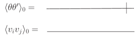
Figure 1: The graphical representation of the propagators of the model.

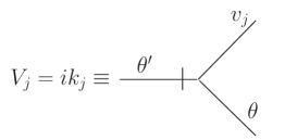
Figure 2: The interaction vertex of the model (wave-number- frequency representation).

The action (III) is given in a form convenient for a realization of the field theoretic perturbation analysis with the standard Feynman diagrammatic technique. From the quadratic part of the action one obtains the matrix of bare propagators. The wave-number-frequency representation of, in what follows, important propagators is as follows: (a) the bare propagator $\langle\theta\theta^{\prime}\rangle_{0}$ defined as

$$\langle\theta\theta^{\prime}\rangle_{0}=\langle\theta^{\prime}\theta\rangle^{*}_{0}=\frac{1}{-i\omega+\nu_{0}k^{2}},$$ (20)

and b) the bare propagator for the velocity field $\langle vv\rangle_{0}$ given directly by Eq. (11), namely,

$$\langle v_{i}v_{j}\rangle_{0}=P^{\rho}_{ij}({\bf k})\tilde{D}^{v}(\omega,k),$$ (21)

where $P^{\rho}_{ij}({\bf k})$ is the transverse projector defined in the previous section by Eq. (6). Their graphical representation is presented in Fig. 1.

The triple (interaction) vertex $-\theta^{\prime}v_{j}\partial_{j}\theta=\theta^{\prime}v_{j}V_{j}\theta$ is present in Fig. 2, where the momentum ${\bf k}$ is flowing into the vertex via the auxiliary field $\theta^{\prime}$.

IV UV renormalization and RG analysis

We start with the analysis of uv divergences, which is usually based on the analysis of canonical dimensions (see, e.g., ZinnJustin ; Vasiliev ; Collins ). First of all, the dynamical model (III), as well as all models of this type, is a so-called two-scale model Vasiliev ; AdAnVa96 ; AdAnVa99 ; AdVaPi83 , i.e., the canonical dimension of some quantity $F$ is described by two numbers, namely, the momentum dimension $d^{k}_{F}$ and the frequency dimension $d^{\omega}_{F}$. To find the dimensions of all quantities it is appropriate to use the standard normalization conditions $d^{k}_{k}=-d^{k}_{x}=1,d^{\omega}_{\omega}=-d^{\omega}_{t}=1,d^{\omega}_{k}=d^{\omega}_{x}=d^{k}_{\omega}=d^{k}_{t}=0$, and the requirement that each term of the action functional must be separately dimensionless with respect to the momentum and frequency dimensions. The total canonical dimension $d_{F}$ is then defined as $d_{F}=d^{k}_{F}+2d^{\omega}_{F}$ [it is related to the fact that $\partial_{t}\propto\nu_{0}\partial^{2}$ in the free action (III) with choice of zero canonical dimension for $\nu_{0}$]. In the framework of the theory of renormalization the total canonical dimension in dynamical models plays the same role as the momentum dimension does in static models.

The canonical dimensions of the model (III) cannot be determined directly because it contains fewer terms than fields and parameters. Thus one is faced with some kind of uncertainty in calculation of canonical dimensions. This freedom is demonstrated by the fact that parameter $h=|{\bf h}|$ can be eliminated from the action (see Ref. Antonov99 for details). When $h$ is eliminated from the action, which is equivalent to the assigning of zero canonical dimension to it, the canonical dimensions of the other quantities can be calculated unambiguously. They are present in Table 1, where also the canonical dimensions of the renormalized parameters are shown.

The model is logarithmic at $\varepsilon=\eta=0$ (the coupling constants $g_{0}$ and $u_{0}$ are dimensionless); therefore the uv divergences in the correlation functions have the form of poles in $\varepsilon,\eta$, and their linear combinations.

The quantity that plays a central role in the renormalization of the model, namely, the role of the formal index of the uv divergence, is the total canonical dimension of an arbitrary one-particle irreducible correlation (Green’s) function $\Gamma=\langle\Phi\cdots\Phi\rangle_{1-ir}$. It is given as follows:

$$d_{\Gamma}=d^{k}_{\Gamma}+2d^{\omega}_{\Gamma}=d+2-N_{\Phi}d_{\Phi},$$ (22)

where $N_{\Phi}=\{N_{\theta},N_{\theta^{\prime}},N_{{\bf v}}\}$ are the numbers of corresponding fields entering into the function $\Gamma$, and summation over all types of fields is implied. It is well known that superficial uv divergences, whose removal requires counterterms, can be present only in those Green’s functions $\Gamma$ for which the total canonical index $d_{\Gamma}$ is a non-negative integer.

A detailed analysis of divergences in the problem (III) was done in Ref. Antonov99 (see also Refs. AdAnVa96 ; AdAnVa99 ); therefore we shall present here only basic facts and conclusions rather than to repeat all details. First of all, every one-irreducible Green’s function with $N_{\theta^{\prime}}<N_{\theta}$ vanishes. On the other hand, dimensional analysis based on Table I leads to the conclusion that for any $d$, superficial divergences can be present only in the one-irreducible Green’s functions $\langle\theta^{\prime}\theta\cdots\theta\rangle$ with only one field $\theta^{\prime}$ ($N_{\theta^{\prime}}=1$) and an arbitrary number $N_{\theta}$ of fields $\theta$. Therefore, in the model under investigation, superficial divergences can be found only in the one-particle irreducible function $\langle\theta^{\prime}\theta\rangle$. To remove them one needs to include into the action functional a counterterm of the form $\theta^{\prime}\triangle\theta$. Its inclusion is manifested by the multiplicative renormalization of the bare parameters $g_{0},u_{0}$, and $\nu_{0}$ in the action functional (III):

$$\nu_{0}=\nu Z_{\nu},\,\,\,g_{0}=g\mu^{2\varepsilon+\eta}Z_{g},\,\,\,u_{0}=u\mu^{\eta}Z_{u}.$$ (23)

Here the dimensionless parameters $g,u$, and $\nu$ are the renormalized counterparts of the corresponding bare ones, $\mu$ is the renormalization mass (a scale setting parameter) in the minimal subtraction (MS) scheme, and $Z_{i}=Z_{i}(g,u)$ are renormalization constants.

Table 1: Canonical dimensions of the fields and parameters of the model under consideration.

$F$	${\bf v}$	$\theta$	$\theta^{\prime}$	$m,\Lambda,\mu$	$\nu_{0},\nu$	$g_{0}$	$u_{0}$	$g,u,h$
$d^{k}_{F}$	-1	-1	$d+1$	1	-2	$2\varepsilon+\eta$	$\eta$	0
$d^{\omega}_{F}$	1	0	0	0	1	0	0	0
$d_{F}$	1	-1	$d+1$	1	0	$2\varepsilon+\eta$	$\eta$	0

The renormalized action functional has the following form:

$$S^{R}(\Phi) = -\frac{1}{2}\int dt_{1}\,d^{d}{\bf x_{1}}\,dt_{2}\,d^{d}{\bf x_{2}}$$

$$v_{i}(t_{1},{\bf x_{1}})[D_{ij}^{v}(t_{1},{\bf x_{1}};t_{2},{\bf x_{2}})]^{-1}v_{j}(t_{2},{\bf x_{2}})$$

$$+ \int dt\,d^{d}{\bf x}\,\,\theta^{\prime}\left[-\partial_{t}\theta-v_{i}\partial_{i}\theta+\nu Z_{1}\triangle\theta-{\bf h}\cdot{\bf v}\right],$$

where the correlator $D_{ij}^{v}$ is written in renormalized parameters (in wave-number-frequency representation)

$$\tilde{D}_{ij}^{v}(\omega,k)=\frac{P^{\rho}_{ij}({\bf k})g\nu^{3}\mu^{2\varepsilon+\eta}k^{4-d-2\varepsilon-\eta}}{(i\omega+u\nu\mu^{\eta}k^{2-\eta})(-i\omega+u\nu\mu^{\eta}k^{2-\eta})}.$$ (25)

By comparison of the renormalized action (IV) with definitions of the renormalization constants $Z_{i}$, $i=g,u,\nu$ [Eq. (23)] we come to the relations among them:

$$Z_{\nu}=Z_{1},\,\,\,Z_{g}=Z_{\nu}^{-3},\,\,\,Z_{u}=Z_{\nu}^{-1}.$$ (26)

The second and third relations are consequences of the absence of the renormalization of the term with $D^{v}$ in the renormalized action (IV). Renormalization of the fields, the mass parameter $m$, and the vector ${\bf h}$ is not needed, i.e., $Z_{\Phi}=1$ for all fields, $Z_{m}=1$, and also $Z_{{\bf h}}=1$.

In what follows, we shall work with two-loop approximation to be able to see the effects of helicity. The calculation of higher-order corrections is more difficult in the models with turbulent velocity field with finite correlation time than in the cases with $\delta$ correlation in time. First of all, one has to calculate more relevant Feynman diagrams in the same order of perturbation theory (see below). A second and more problematic distinction is related to the fact that the diagrams for the finite correlated case involve two different dispersion laws, namely, $\omega\propto k^{2}$ for the scalar field and $\omega\propto k^{2-\eta}$ for the velocity field. This leads to complicated expressions for renormalization constants even in the simplest (one-loop) approximation Antonov99 ; Antonov00 . But, as was discussed in Antonov99 ; Antonov00 ; AdAnHo02 , this difficulty can be avoided by the calculation of all renormalization constants in an arbitrary specific choice of the exponents $\varepsilon$ and $\eta$ that guarantees uv finiteness of the Feynman diagrams. From the point of calculations the most suitable choice is to put $\eta=0$ and leave $\varepsilon$ arbitrary.

Thus, the knowledge of the renormalization constants for the special choice $\eta=0$ is sufficient to obtain all important quantities like the $\gamma$-functions, $\beta$-functions, coordinates of fixed points, and critical dimensions.

This possibility is not automatic in general. In the model under consideration it is the consequence of an analysis which shows that in the MS scheme all the needed anomalous dimensions are independent of the exponents $\varepsilon$ and $\eta$ in the two-loop approximation. But in the three-loop approximation they can simply appear AdAnHo02 .

In Ref. AdAnHo02 the two-loop corrections to the anomalous exponents of model (III) without helicity were studied. We shall continue those investigations including the effects of helicity.

Now we can continue with renormalization of the model. The relation $S(\theta,\theta^{\prime},{\bf v},e_{0})=S^{R}(\theta,\theta^{\prime},{\bf v},e,\mu)$, where $e_{0}$ stands for the complete set of bare parameters and $e$ stands for the renormalized ones, leads to the relation $W(A,e_{0})=W^{R}(A,e,\mu)$ for the generating functional of connected Green’s functions. By application of the operator $\tilde{\cal{D}}_{\mu}\equiv\mu\partial_{\mu}$ at fixed $e_{0}$ on both sides of the last equation one obtains the basic RG differential equation

$${\cal{D}}_{RG}W^{R}(A,e,\mu)=0,$$ (27)

where ${\cal{D}}_{RG}$ represents the operation $\tilde{\cal{D}}_{\mu}$ written in the renormalized variables. Its explicit form is

$${\cal{D}}_{RG}={\cal{D}}_{\mu}+\beta_{g}(g,u)\partial_{g}+\beta_{u}(g,u)\partial_{u}-\gamma_{\nu}(g,u){\cal{D}}_{\nu},$$ (28)

where we denote ${\cal{D}}_{x}\equiv x\partial_{x}$ for any variable $x$ and the RG functions (the $\beta$ and $\gamma$ functions) are given by well-known definitions, and in our case, using relations (26) for renormalization constants, they have the following form

$$\gamma_{\nu} \equiv \tilde{\cal{D}}_{\mu}\ln Z_{\nu},$$ (29)

$$\beta_{g} \equiv \tilde{\cal{D}}_{\mu}g=g(-2\varepsilon-\eta+3\gamma_{\nu}),$$ (30)

$$\beta_{u} \equiv \tilde{\cal{D}}_{\mu}u=u(-\eta+\gamma_{\nu}).$$ (31)

The renormalization constant $Z_{\nu}$ is determined by the requirement that the one-irreducible Green’s function $\langle\theta^{\prime}\theta\rangle_{1-ir}$ must be uv finite when is written in renormalized variables. In our case it means that they have no singularities in the limit $\varepsilon,\eta\rightarrow 0$. The one-irreducible Green’s function $\langle\theta^{\prime}\theta\rangle_{1-ir}$ is related to the self-energy operator $\Sigma_{\theta^{\prime}\theta}$ by the Dyson equation

$$\langle\theta^{\prime}\theta\rangle_{1-ir}=-i\omega+\nu_{0}p^{2}-\Sigma_{\theta^{\prime}\theta}(\omega,p).$$ (32)

Thus $Z_{\nu}$ is found from the requirement that the uv divergences are canceled in Eq. (32) after the substitution $\nu_{0}=\nu Z_{\nu}$. This determines $Z_{\nu}$ up to an uv-finite contribution, which is fixed by the choice of the renormalization scheme. In the MS scheme all the renormalization constants have the form (1 + poles in $\varepsilon,\eta$ and their linear combinations). The self-energy operator $\Sigma_{\theta^{\prime}\theta}$ is represented by the corresponding one-irreducible diagrams. In contrast to the rapid-change model, where only the one-loop diagram exists (it is related to the fact that all higher-loop diagrams contain at least one closed loop that is built up of only retarded propagators and thus are automatically equal to zero), in the case with finite correlations in time of the velocity field, higher-order corrections are nonzero. In two-loop approximation the self-energy operator $\Sigma_{\theta^{\prime}\theta}$ is defined by diagrams that are shown in Fig. 3.

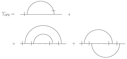
Figure 3: The one and two-loop diagrams that contribute to the self-energy operator $\Sigma_{\theta^{\prime}\theta}$.

As was already mentioned, in our calculations we can put $\eta=0$. This possibility essentially simplifies the evaluations of all quantities Antonov99 ; Antonov00 ; AdAnHo02 . Then the singular parts of the diagrams in Fig. 3 have the following analytical form (for calculational details see Appendix A):

$$A = -\frac{S_{d}}{(2\pi)^{d}}\frac{g\nu p^{2}}{4u(1+u)}\frac{d-1}{d}\left(\frac{\mu}{m}\right)^{2\varepsilon}\frac{1}{\varepsilon},$$ (33)

$$B_{1} = \frac{S_{d}^{2}}{(2\pi)^{2d}}\frac{g^{2}\nu p^{2}}{16u^{2}(1+u)^{3}}\frac{(d-1)^{2}}{d^{2}}\left(\frac{\mu}{m}\right)^{4\varepsilon}$$

$$\times \frac{1}{\varepsilon}\left(\frac{1}{2\varepsilon}+\frac{{{}_{2}F_{1}}\left(1,1;2+\frac{d}{2};\frac{1}{(1+u)^{2}}\right)}{(d+2)(1+u)^{2}}\right),$$ (34)

$$B_{2} = \frac{S_{d}^{2}}{(2\pi)^{2d}}\frac{g^{2}\nu p^{2}}{16u^{2}(1+u)^{3}}\frac{(d-1)}{d^{2}}\left(\frac{\mu}{m}\right)^{4\varepsilon}\frac{1}{\varepsilon}$$

$$\times \Bigg{[}\frac{{{}_{2}F_{1}}\left(1,1;2+\frac{d}{2};\frac{1}{(1+u)^{2}}\right)}{(d+2)(1+u)}$$

$$-\frac{(d-2)\pi\rho^{2}}{2}\,{{}_{2}F_{1}}\left(\frac{1}{2},\frac{1}{2};1+\frac{d}{2};\frac{1}{(1+u)^{2}}\right)\Bigg{]},$$

Expression $A$ is the result of the one-loop diagram, $B_{1}$ is the result for the first two-loop diagram (the first diagram in the second row in Fig. 3), and $B_{2}$ is the result for the second two-loop graph (the second diagram in the second row in Fig. 3). Here, $S_{d}=2\pi^{d/2}/\Gamma(d/2)$ denotes the $d$-dimensional sphere, ${{}_{2}F_{1}}(a,b,c,z)=1+\frac{a\,b}{c\cdot 1}z+\frac{a(a+1)b(b+1)}{c(c+1)\cdot 1\cdot 2}z^{2}+\ldots$ represents the corresponding hypergeometric function. In further investigations the helical term with $\rho^{2}$ in $B_{2}$ has to be taken with $d=3$ but for completeness we leave the $d$ dependence in this part of $B_{2}$ in Eq. (IV).

Finally, the renormalization constant $Z_{\nu}=Z_{1}$ is given as follows:

$$Z_{\nu}=1 - \frac{\bar{g}}{\varepsilon}\frac{d-1}{d}\frac{1}{4u(1+u)}-\frac{\bar{g}^{2}}{\varepsilon^{2}}\frac{(d-1)^{2}}{d^{2}}\frac{1}{32u^{2}(1+u)^{3}}$$

$$+ \frac{\bar{g}^{2}}{\varepsilon}\frac{(d-1)(d+u)}{d^{2}(d+2)}\frac{1}{16u^{2}(1+u)^{5}}$$

$$\times\,{{}_{2}F_{1}}\left(1,1;2+\frac{d}{2};\frac{1}{(1+u)^{2}}\right)$$

$$- \rho^{2}\frac{\bar{g}^{2}}{\varepsilon}\frac{\pi}{144u^{2}(1+u)^{3}}\,{{}_{2}F_{1}}\left(\frac{1}{2},\frac{1}{2};\frac{5}{2};\frac{1}{(1+u)^{2}}\right),$$

where in the helical part (the last line) we already substitute $d=3$ and denote $\bar{g}=gS_{d}/(2\pi)^{d}$.

Now using the definition of the anomalous dimension $\gamma_{\nu}$ in Eq. (29) one comes to the following expression:

$$\gamma_{\nu}=-2(\bar{g}{\cal A}+2\bar{g}^{2}{\cal B}),$$ (37)

where

$${\cal A}=-\frac{d-1}{d}\frac{1}{4u(1+u)}$$ (38)

is the one-loop contribution to the anomalous dimension $\gamma_{\nu}$ and the two-loop contribution is

$${\cal B} = \frac{(d-1)(d+u)}{16d^{2}(d+2)u^{2}(1+u)^{5}}\,{{}_{2}F_{1}}\left(1,1;2+\frac{d}{2};\frac{1}{(1+u)^{2}}\right)$$ (39)

$$-\frac{\pi\rho^{2}}{144u^{2}(1+u)^{3}}\,{{}_{2}F_{1}}\left(\frac{1}{2},\frac{1}{2};\frac{5}{2};\frac{1}{(1+u)^{2}}\right).$$

The issues of interest are especially the multiplicatively renormalizable equal-time two-point quantities $G(r)$ (see, e.g., Ref. Antonov99 ). Examples of such quantities are the equal-time structure functions

$$S_{n}(r)\equiv\langle[\theta(t,{\bf x})-\theta(t,{\bf x^{\prime}})]^{n}\rangle$$ (40)

in the inertial range, specified by the inequalities $l\sim 1/\Lambda\ll r\ll L=1/m$ ($l$ is an internal length). Here the angular brackets $\langle\cdots\rangle$ mean the functional average over fields $\Phi=\{\theta,\theta^{\prime},{\bf v}\}$ with weight $\exp S^{R}(\Phi).$ The infrared (ir) scaling behavior of the function $G(r)$ (for $r/l\gg 1$ and any fixed $r/L$)

$$G(r)\simeq\nu_{0}^{d^{\omega}_{G}}l^{-d_{G}}(r/l)^{-\Delta_{G}}R(r/L)$$ (41)

is related to the existence of ir stable fixed points of the RG equations (see the next section). In (41) $d^{\omega}_{G}$ and $d_{G}$ are corresponding canonical dimensions of the function $G$, $R(r/L)$ is the so-called scaling function, which cannot be determined by the RG equation (see, e.g., Ref. Vasiliev ), and $\Delta_{G}$ is the critical dimension defined as

$$\Delta_{G}=d_{G}^{k}+\Delta_{\omega}d_{G}^{\omega}+\gamma_{G}^{*}.$$ (42)

Here $\gamma_{G}^{*}$ is the fixed point value of the anomalous dimension $\gamma_{G}\equiv\mu\partial_{\mu}\ln Z_{G}$, where $Z_{G}$ is the renormalization constant of the multiplicatively renormalizable quantity $G$, i.e., $G=Z_{G}G^{R}$ Antonov00 , and $\Delta_{\omega}=2-\gamma_{\nu}^{*}$ is the critical dimension of the frequency with $\gamma_{\nu}$ which is defined in Eq. (37) (see also the next section).

On the other hand, the small-$r/L$ behavior of the scaling function $R(r/L)$ can be studied using the Wilson OPE Vasiliev . It shows that, in the limit $r/L\to 0$, the function $R(r/L)$ can be written in the following asymptotic form

$$R(r/L)=\sum_{F}C_{F}(r/L)\,(r/L)^{\Delta_{F}},$$ (43)

where $C_{F}$ are coefficients regular in $r/L$. In general, summation is implied over certain renormalized composite operators $F$ with critical dimensions $\Delta_{F}$. In the case under consideration the leading contribution is given by operators $F$ having the form $F_{n}=(\partial_{i}\theta\partial_{i}\theta)^{n}.$ In Sec. VII we shall consider them in detail where the complete two-loop calculation of the critical dimensions of the composite operators $F_{n}$ will be presented for arbitrary values of $n$, $d$, $u$, and $\rho$.

V Fixed points and scaling regimes

Possible scaling regimes of a renormalizable model are directly given by the ir stable fixed points of the corresponding system of RG equations ZinnJustin ; Vasiliev . The fixed point of the RG equations is defined by $\beta$-functions, namely, by the requirement of their vanishing. In our model, the coordinates $g_{*},u_{*}$ of the fixed points are found from the system of two equations

$$\beta_{g}(g_{*},u_{*})=\beta_{u}(g_{*},u_{*})=0.$$ (44)

The beta functions $\beta_{g}$ and $\beta_{u}$ are defined in Eqs. (30) and (31). To investigate the ir stability of a fixed point it is enough to analyze the eigenvalues of the matrix $\Omega$ of first derivatives:

$$\Omega_{ij}=\left(\begin{array}[]{cc}\partial\beta_{g}/\partial g&\partial\beta_{g}/\partial u\\ \partial\beta_{u}/\partial g&\partial\beta_{u}/\partial u\end{array}\right).$$ (45)

The ir asymptotic behavior is governed by the ir stable fixed points, i.e., those for which both eigenvalues are positive.

Figure 4: Regions of stability for the fixed points in one-loop approximation. The regions of stability for fixed points FPI, FPII, and FPIII are exact, i.e., not influenced by loop corrections. The fixed point FPIV is shown in one-loop approximation. The $d$ dependence of the FPIV in two-loop approximation is shown in Fig. 5 below.

The possible scaling regimes of the model in one-loop approximation were investigated in Ref. Antonov99 . Our first question is how the two-loop approximation changes the picture of the ”phase” diagram of scaling regimes discussed in Ref. Antonov99 , and the second one is what restrictions on this picture are given by helicity (in the two-loop approximation). The two-loop approximation in the model under our consideration without helicity was studied in Ref. AdAnHo02 but the question of scaling regimes from the two-loop approximation point of view was not discussed in detail.

Figure 5: Regions of stability for the fixed point FPIV in the two-loop approximation without helicity for different space dimensions $d$. The ir fixed point is stable in the region given by the inequalities $\varepsilon>0,\varepsilon>\eta$, and $\varepsilon<d-1$.

First of all, we shall study the rapid-change limit $u\rightarrow\infty$. In this regime, it is convenient to make a transformation to new variables, namely, $w\equiv 1/u$ and $g^{\prime}\equiv g/u^{2}$, with the corresponding changes in the $\beta$ functions:

$$\beta_{g^{\prime}} = g^{\prime}(\eta-2\varepsilon+\gamma_{\nu}),$$ (46)

$$\beta_{w} = w(\eta-\gamma_{\nu}).$$ (47)

In this notation the anomalous dimension $\gamma_{\nu}$ obtains the following form:

$$\gamma_{\nu}=-2(\bar{g}^{\prime}{\cal A^{\prime}}+2\bar{g}^{\prime 2}{\cal B^{\prime}}),$$ (48)

where again $\bar{g}^{\prime}=g^{\prime}S_{d}/(2\pi)^{d}$. The one-loop contribution ${\cal A^{\prime}}$ acquires the form

$${\cal A^{\prime}}=-\frac{d-1}{d}\frac{1}{4(1+w)}$$ (49)

and the two-loop correction ${\cal B^{\prime}}$ is

$${\cal B^{\prime}} = \frac{(d-1)(dw+1)w^{2}}{16d^{2}(d+2)(1+w)^{5}}\,{{}_{2}F_{1}}\left(1,1;2+\frac{d}{2};\frac{w^{2}}{(1+w)^{2}}\right)$$ (50)

$$-\frac{\pi\rho^{2}w}{144(1+w)^{3}}\,{{}_{2}F_{1}}\left(\frac{1}{2},\frac{1}{2};\frac{5}{2};\frac{w^{2}}{(1+w)^{2}}\right).$$

It is evident that in the rapid-change limit $w\rightarrow 0$ ($u\rightarrow\infty$) the two-loop contribution ${\cal B^{\prime}}$ is equal to zero. This is not surprising because in the rapid-change model there are no higher-loop corrections to the self-energy operator AdAnVa98+ ; AdAnBaKaVa01 ; thus we are coming to the one-loop result of Ref. Antonov99 with the anomalous dimension $\gamma_{\nu}$ of the form

$$\gamma_{\nu}=\lim_{w\rightarrow 0}\frac{(d-1){\bar{g}^{\prime}}}{2d(1+w)}=\frac{(d-1){\bar{g}^{\prime}}}{2d}$$ (51)

In this regime we have two fixed points denoted as FPI and FPII in Ref. Antonov99 . The first fixed point is trivial, namely,

$$\mathrm{FPI}:\,\,\,\,w_{*}=g_{*}^{\prime}=0,$$ (52)

with $\gamma_{\nu}^{*}=0$, and diagonal matrix $\Omega$ with eigenvalues (diagonal elements)

$$\Omega_{1}=\eta,\,\,\,\,\,\Omega_{2}=\eta-2\varepsilon.$$ (53)

The region of stability is shown in Fig. 4. The second point is defined as

$$\mathrm{FPII}:\,\,\,\,w_{*}=0,\,\,\,\bar{g}_{*}^{\prime}=\frac{2d}{d-1}(2\varepsilon-\eta),$$ (54)

with $\gamma_{\nu}^{*}=2\varepsilon-\eta$. These are exact one-loop expressions as a result of the nonexistence of the higher-loop corrections [see discussion below (50)]. That means that they have no corrections of order $O(\varepsilon^{2})$ and higher [we work with the assumption that $\varepsilon\simeq\eta$; therefore it also includes corrections of the type $O(\eta^{2})$ and $O(\eta\varepsilon)$]. The corresponding ”stability matrix” is triangular with diagonal elements (eigenvalues)

$$\Omega_{1}=2(\eta-\varepsilon),\,\,\,\,\Omega_{2}=2\varepsilon-\eta.$$ (55)

The region of stability of this fixed point is shown in Fig. 4.

Now let us analyze the ”frozen regime” with frozen velocity field, which is mathematically obtained from the model under consideration in the limit $u\rightarrow 0$. To study this transition it is appropriate to change the variable $g$ to the new variable $g^{\prime\prime}\equiv g/u$ Antonov99 . Then the $\beta$ functions are transformed to the following:

$$\beta_{g^{\prime\prime}} = g^{\prime\prime}(-2\varepsilon+2\gamma_{\nu}),$$ (56)

$$\beta_{u} = u(-\eta+\gamma_{\nu}),$$ (57)

where the $\beta_{u}$ function is not changed, i.e., it is the same as the initial one (31). In this notation the anomalous dimension $\gamma_{\nu}$ has the form

$$\gamma_{\nu}=-2(\bar{g}^{\prime\prime}{\cal A^{\prime\prime}}+2\bar{g}^{\prime\prime 2}{\cal B^{\prime\prime}}),$$ (58)

where, as obvious, $\bar{g}^{\prime\prime}=g^{\prime\prime}S_{d}/(2\pi)^{d}$. The one-loop part ${\cal A^{\prime\prime}}$ is now defined as

$${\cal A^{\prime\prime}}=-\frac{d-1}{d}\frac{1}{4(1+u)}$$ (59)

and the two-loop one ${\cal B^{\prime\prime}}$ is given by

$${\cal B^{\prime\prime}} = \frac{(d-1)(d+u)}{16d^{2}(d+2)(1+u)^{5}}\,{{}_{2}F_{1}}\left(1,1;2+\frac{d}{2};\frac{1}{(1+u)^{2}}\right)$$ (60)

$$-\frac{\pi\rho^{2}}{144(1+u)^{3}}\,{{}_{2}F_{1}}\left(\frac{1}{2},\frac{1}{2};\frac{5}{2};\frac{1}{(1+u)^{2}}\right).$$

In the limit $u\rightarrow 0$ the functions ${\cal A^{\prime\prime}}$ and ${\cal B^{\prime\prime}}$ obtain the following forms

$${\cal A^{\prime\prime}}_{0}=-\frac{d-1}{4d}$$ (61)

and

$${\cal B^{\prime\prime}}_{0}=\frac{(d-1){{}_{2}F_{1}}\left(1,1;2+\frac{d}{2};1\right)}{16d(d+2)}-\frac{\pi\rho^{2}{{}_{2}F_{1}}\left(\frac{1}{2},\frac{1}{2};\frac{5}{2};1\right)}{144}.$$ (62)

The system of $\beta$ functions (56) and (57) exhibits two fixed points, denoted as FPIII and FPIV in Ref. Antonov99 , related to the corresponding two scaling regimes. One of them is trivial,

$$\mathrm{FPIII}:\,\,\,\,u_{*}=g_{*}^{\prime\prime}=0,$$ (63)

with $\gamma_{\nu}^{*}=0$. The eigenvalues of the corresponding matrix $\Omega$, which is diagonal in this case, are

$$\Omega_{1}=-2\varepsilon,\,\,\,\,\Omega_{2}=-\eta.$$ (64)

Thus, this regime is ir stable only if both parameters $\varepsilon$ and $\eta$ are negative simultaneously as can be seen in Fig. 4. The second, nontrivial, point is

$$\mathrm{FPIV}:\,\,\,\,u_{*}=0,\,\,\,\,\bar{g}_{*}^{\prime\prime}=-\frac{\varepsilon}{2{\cal A^{\prime\prime}}_{0}}-\frac{{\cal B^{\prime\prime}}_{0}}{2{\cal A^{\prime\prime}}_{0}^{2}}\varepsilon^{2},$$ (65)

where ${\cal A^{\prime\prime}}_{0}$ and ${\cal B^{\prime\prime}}_{0}$ are defined in Eqs. (61) and (62), respectively.

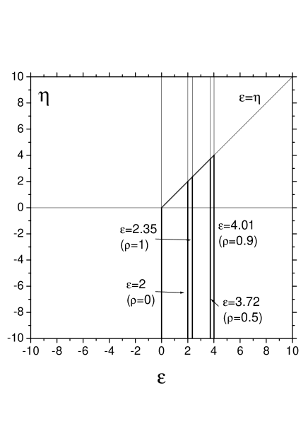
Figure 6: Regions of the stability for the fixed point FPIV in two-loop approximation with helicity. The ir fixed point is stable in the region given by the inequalities $\varepsilon>0,\varepsilon>\eta$, and $\varepsilon<\varepsilon_{\rho}$.

Figure 7: Regions of stability for the fixed point FPV in the two-loop approximation without helicity. $d$ dependence of the stability is shown.

First, let us study the influence of the two-loop approximation on this ir scaling regime without helicity in the general $d$-dimensional case. We denote the corresponding fixed point as FPIV₀, and its coordinates are

$$\mathrm{FPIV_{0}}:\,\,\,u_{*}=0,\,\,\,\,\bar{g}_{*}^{\prime\prime}=\frac{2d}{d-1}\left(\varepsilon+\frac{1}{d-1}\varepsilon^{2}\right),$$ (66)

with anomalous dimension $\gamma_{\nu}$ defined as

$$\gamma_{\nu}^{*}=\frac{d-1}{2d}\left(\bar{g}_{*}^{\prime\prime}-\frac{\bar{g}_{*}^{\prime\prime 2}}{2d}\right)=\varepsilon,$$ (67)

which is the exact one-loop result Antonov99 . The eigenvalues of the matrix $\Omega$ (taken at the fixed point) are

$$\Omega_{1}=2\left(\varepsilon+\frac{1}{1-d}\varepsilon^{2}\right),\,\,\,\Omega_{2}=\varepsilon-\eta.$$ (68)

The eigenvalue $\Omega_{2}=\partial_{u}\beta_{u}|_{*}=-\eta+\gamma_{\nu}^{*}$ is also an exact one-loop result. The conditions $\bar{g}_{*}^{\prime\prime}>0,\Omega_{1}>0$, and $\Omega_{2}>0$ for the ir-stable fixed point lead to the following restrictions on the values of the parameters $\varepsilon$ and $\eta$:

$$\varepsilon>0,\,\,\,\varepsilon>\eta,\,\,\,\varepsilon<d-1.$$ (69)

The region of stability is shown in Fig. 5. The region of stability of this ir fixed point increases when the dimension of the coordinate space $d$ increases.

Now turn to the system with helicity. In this case the dimension of the space is fixed for $d=3$. Thus, our starting conditions for a stable ir fixed point of this type are obtained from the conditions (69) with the explicit value d=3: $\varepsilon>0,\varepsilon>\eta,\varepsilon<2$. But they are valid only if helicity is vanishing and could be changed when nonzero helicity is present. Let us study this case. When helicity is present the fixed point FPIV is given as

$$u_{*}=0,\,\,\,\,\bar{g}_{*}^{\prime\prime}=3\varepsilon+\frac{3}{2}\left(1-\frac{3\pi^{2}\rho^{2}}{16}\right)\varepsilon^{2},$$ (70)

Therefore, in the helical case, the situation is a little bit more complicated as a result of the competition between nonhelical and helical terms within two-loop corrections. The matrix $\Omega$ is triangular with diagonal elements (taken already at the fixed point)

$$\Omega_{1} = 2\varepsilon+\left(-1+\frac{3\pi^{2}\rho^{2}}{16}\right)\varepsilon^{2},$$ (71)

$$\Omega_{2} = \varepsilon-\eta,$$ (72)

where explicit dependence of the eigenvalue $\Omega_{1}$ on the parameter $\rho$ occures. The requirement to have positive values for the parameter $\bar{g}_{*}^{\prime\prime}$, and at the same time for the eigenvalues $\Omega_{1},\Omega_{2}$ leads to the region of the stable fixed point. The results are shown in Fig. 6. The picture is rather complicated due to the very existence of the critical absolute value of $\rho$

$$\rho_{c}=\frac{4}{\sqrt{3}\pi},$$ (73)

which is defined from the condition of vanishing of the two-loop corrections in Eqs. (70) and (71):

$$\left(-1+\frac{3\pi^{2}\rho^{2}}{16}\right)=0.$$ (74)

As was already discussed above, when helicity is not present, the system exhibits this type of fixed point (and, of course, the corresponding scaling behavior) in the region restricted by the inequalities $\varepsilon>0,\varepsilon>\eta$, and $\varepsilon<2$. The last condition changes when the helicity is switched on. The important feature here is that the two-loop contributions to $\bar{g}_{*}^{\prime\prime}$ and $\Omega_{1}$ have the same structure but opposite sign. This leads to different sources of conditions in the cases when $|\rho|<\rho_{c}$ and $|\rho|>\rho_{c}$, respectively. In the situation with $|\rho|<\rho_{c}$ the positiveness of $\Omega_{1}$ plays a crucial role and one has the following region of stability of the ir-fixed point FPIV:

$$\varepsilon>0,\,\,\,\varepsilon>\eta,\,\,\,\varepsilon<\frac{32}{16-3\pi^{2}\rho^{2}}.$$ (75)

On the other hand, in the case with $|\rho|>\rho_{c}$, the principal restriction on the ir-stable regime is yielded by the condition $\bar{g}_{*}^{\prime\prime}>0$ with final ir-stable region defined as

$$\varepsilon>0,\,\,\,\varepsilon>\eta,\,\,\,\varepsilon<\frac{32}{-16+3\pi^{2}\rho^{2}}.$$ (76)

Therefore, if we continuously increase the absolute value of the helicity parameter $\rho$, the region of stability of the fixed point defined by the last inequality in Eq. (75) increases too. This restriction vanishes completely when $|\rho|$ reaches the critical value $\rho_{c}$, and the picture becomes the same as in the one-loop approximation Antonov99 . In this rather specific situation the two-loop influence on the region of stability of the fixed point is exactly zero: the helical and nonhelical two-loop contributions are canceled by each other. Then if the absolute value of the parameter $\rho$ increases further, the last condition appears again, namely, the third condition in Eq. (76), and the restriction becomes stronger when $|\rho|$ tends to its maximal value, $|\rho|=1$. In this case of the maximal breaking of mirror symmetry (maximal helicity), $|\rho|=1$, the region of the ir stability of the fixed point is defined by the inequalities $\varepsilon>0,\varepsilon=\eta$, and $\varepsilon<2.351$ (see Fig. 6). It is interesting that the presence of helicity in the system leads to the enlargement of the stability region.

Figure 8: Regions of stability for the fixed point FPV in the two-loop approximation with helicity in the situation when $\rho<\rho_{c}=4/(3^{1/2}\pi)$.

Now let us turn to the most interesting scaling regime with a finite value of the fixed point for the variable $u$. But by a short analysis one immediately concludes that the system of equations (see also Antonov99 )

$$\beta_{g} = g(-2\varepsilon-\eta+3\gamma_{\nu})=0,$$ (77)

$$\beta_{u} = u(-\eta+\gamma_{\nu})=0$$ (78)

can be satisfied simultaneously for finite values of $g,u$ only in the case when the parameter $\varepsilon$ is equal to $\eta$: $\varepsilon=\eta$. In this case, the function $\beta_{g}$ is proportional to the function $\beta_{u}$. As a result we have not one fixed point of this type but a curve of fixed points in the $g-u$ plane. The value of the fixed point for the variable $g$ in the two-loop approximation is given as follows (we denote it as in Ref. Antonov99 as FPV):

$$\mathrm{FPV}:\,\,\,\bar{g}_{*}=-\frac{1}{2{\cal A}_{*}}\,\,\varepsilon-\frac{1}{2}\frac{{\cal B}_{*}}{{\cal A}_{*}^{3}}\,\,\varepsilon^{2},$$ (79)

with the exact one-loop result for $\gamma_{\nu}^{*}=\varepsilon=\eta$ [this is already directly given by Eq. (78)]. Here ${\cal A}_{*}$ and ${\cal B}_{*}$ are expressions ${\cal A}$ and ${\cal B}$ from Eqs. (38) and (39) which are taken at the fixed point value $u_{*}$ of the variable $u$. The possible values of the fixed point for the variable $u$ can be restricted (and will be restricted) as we shall discuss below. The stability matrix $\Omega$ has the following eigenvalues:

$$\Omega_{1}=0,\,\,\,\Omega_{2}=3\bar{g}^{*}\left(\frac{\partial\gamma_{\nu}}{\partial g}\right)_{*}+u^{*}\left(\frac{\partial\gamma_{\nu}}{\partial u}\right)_{*}.$$ (80)

The vanishing of $\Omega_{1}$ is an exact result which is related to the degeneracy of the system of Eqs. (77) and (78) when nonzero solutions with respect to $g$ and $u$ are assumed, or, equivalently, it reflects the existence of a marginal direction in the $g-u$ plane along the line of fixed points.

Figure 9: Regions of the stability for the fixed point FPV in two-loop approximation with helicity in the situation when $\rho\geq\rho_{c}=4/(3^{1/2}\pi)$.

We start the analysis of the last fixed point with the investigation of the influence of the two-loop correction on the corresponding scaling regime when helicity is not present in the system ($\rho=0$). In this situation it is interesting to determine the dependence of the scaling regime on dimension $d$. The coordinates of the possible fixed points are

$$\bar{g}_{*} = \frac{2du_{*}(1+u_{*})}{d-1}\varepsilon$$ (81)

$$+ \frac{2du_{*}(d+u_{*}){{}_{2}F_{1}}\left(1,1;2+\frac{d}{2};\frac{1}{(1+u_{*})^{2}}\right)}{(d-1)^{2}(d+2)(1+u_{*})^{2}}\varepsilon^{2},$$

where $u_{*}$ is arbitrary for now. To have a positive value of the fixed point for variables $g$ and $u$ one finds a restriction on the parameter $\varepsilon$: $\varepsilon>0$. Possible restrictions on the ir fixed point value of the variable $u$ can be found from the condition $\Omega_{2}>0$. The explicit form of $\Omega_{2}$ is

$$\Omega_{2} = \frac{2+u_{*}}{1+u_{*}}\varepsilon+\frac{\varepsilon^{2}}{(d-1)(d+2)(d+4)(1+u_{*})^{6}}$$

$$\times \bigg{(}(1+u_{*})^{2}(4+d)(2d(u_{*}-1)+(u_{*}-3)u_{*})$$

$$\,\,\,\,\ \times\,\,{{}_{2}F_{1}}\left(1,1;2+\frac{d}{2};\frac{1}{(1+u_{*})^{2}}\right)$$

$$+4u_{*}(d+u_{*}){{}_{2}F_{1}}\left(2,2;3+\frac{d}{2};\frac{1}{(1+u_{*})^{2}}\right)\bigg{)}.$$

In Fig. 7, the regions of stability for the fixed point FPV without helicity in the $\varepsilon-u$ plane for different space dimensions $d$ are shown. It is interesting that in the two-loop case a nontrivial $d$ dependence of ir stability appears, in contrast to the one-loop approximation Antonov99 .

Now let us turn to the situation with helicity and investigate its influence on the stability of the ir fixed point. In this case we work in three-dimensional space; thus the coordinates of the fixed point are defined by the following equation:

$$\bar{g}_{*} = 3u_{*}(1+u_{*})\varepsilon+\frac{3u_{*}\varepsilon^{2}}{20(1+u_{*})^{2}}$$

$$\times \bigg{(}2(3+u_{*}){{}_{2}F_{1}}\left(1,1;\frac{7}{2};\frac{1}{(1+u_{*})^{2}}\right)$$

$$-5\pi(1+u_{*})^{2}\rho^{2}{{}_{2}F_{1}}\left(\frac{1}{2},\frac{1}{2};\frac{5}{2};\frac{1}{(1+u_{*})^{2}}\right)\bigg{)}.$$

The competition between helical and nonhelical terms appears again, which will lead to a nontrivial restriction for the fixed point values of the variable $u$ to have positive fixed values for variable $g$. Next, the eigenvalue $\Omega_{2}$ of the matrix $\Omega$ is now

$$\Omega_{2} = \frac{2+u_{*}}{1+u_{*}}\varepsilon+\frac{\varepsilon^{2}}{140(1+u_{*})^{6}}$$ (84)

$$\times \bigg{[}8u(3+u){{}_{2}F_{1}}\left(2,2;\frac{9}{2};\frac{1}{(1+u_{*})^{2}}\right)$$

$$\,\,\,\,+14(1+u_{*})^{2}(u_{*}(3+u_{*})-6)$$

$$\,\,\,\,\,\,\,\,\,\,\times\,{{}_{2}F_{1}}\left(1,1;\frac{7}{2};\frac{1}{(1+u_{*})^{2}}\right)$$

$$\,\,\,\,\,+7\pi\rho^{2}(1+u_{*})^{2}$$

$$\,\,\,\,\,\,\times\bigg{(}10(1+u_{*})^{2}\left(\frac{1}{2},\frac{1}{2};\frac{5}{2};\frac{1}{(1+u_{*})^{2}}\right)$$

$$\,\,\,\,\,\,\,\,\,\,\,\,-u_{*}\left(\frac{3}{2},\frac{3}{2};\frac{7}{2};\frac{1}{(1+u_{*})^{2}}\right)\bigg{)}\bigg{]}$$

with a nontrivial helical part that plays an important role in determination of the region of ir stability of the fixed point.

It cannot be seen immediately from Eqs. (V) and (84) but numerical analysis shows that again an important role is played by $\rho_{c}=4/(\sqrt{3}\pi)$. First let us study the case when $|\rho|<\rho_{c}$. The corresponding region of stable ir fixed points with $g_{*}>0$ is shown in Fig. 8. In the case when helicity is not present ($\rho=0$, see the corresponding curve in Fig. 8), the only restriction is given by the condition that $\Omega_{2}>0$; on the other hand, the condition $g_{*}>0$ is satisfied without restriction on the parameter space. When arbitrarily small helicity is present, i.e., $\rho>0$, a restriction related to positiveness of $g_{*}$ arises and is stronger when $|\rho|$ is increasing (the right curve for the concrete value of $\rho$ in Fig. 8) and comes to play the dominant role. At the same time, with increasing of $|\rho|$ the importance of the positiveness of the eigenvalue $\Omega_{2}$ decreases (the left curve for the concrete value of $\rho$ in Fig. 8). For a given $|\rho|<\rho_{c}$ there exists an interval of values of the variable $u_{*}$ for which there is no restriction on the value of the parameter $\varepsilon$. For example, for $|\rho|=0.1$, it is $1.128<u_{*}<13.502$, for $|\rho|=0.5$, $0.217<u_{*}<0.394$, and for $|\rho|=0.7$, $0.019<u_{*}<0.029$. Now turn to the case $|\rho|\geq\rho_{c}$. When $|\rho|$ acquires its critical value $\rho_{c}$, the ir fixed point is stable for all values of $u_{*}>0$ and $\varepsilon>0$, i.e., the condition $\Omega_{2}>0$ becomes satisfied without restrictions on the parameter space. On the other hand, the condition $g_{*}>0$ yields a strong enough restriction and it becomes stronger when $|\rho|$ tends to its maximal value $|\rho|=1$ as it can be seen in Fig. 9).

The most important conclusion of our two-loop investigation of the model is the fact that the possible restrictions on the regions of stability of ir fixed points are ”pressed” to the region with rather large values of $\epsilon$, namely, $\varepsilon\geq 2$, and do not disturb the regions with relatively small $\varepsilon$. For example, the Kolmogorov point ($\varepsilon=\eta=4/3$) is not influenced.

As was already discussed (see the previous section) if $F$ denotes some multiplicatively renormalized quantity (a parameter, a field, or a composite operator) then its critical dimension is given by the expression

$$\Delta[F]\equiv\Delta_{F}=d_{F}^{k}+\Delta_{\omega}d_{F}^{\omega}+\gamma^{*}_{F}\,,$$ (85)

see, e.g., Refs. AdAnVa96 ; AdAnVa99 ; Vasiliev for details. In Eq. (85) $d_{F}^{k}$ and $d_{F}^{\omega}$ are the canonical dimensions of $F$, $\Delta_{\omega}=2-\gamma^{*}_{\nu}$ is the critical dimension of frequency, and $\gamma^{*}_{F}$ is the value of the anomalous dimension $\gamma_{F}\equiv\tilde{\cal D}_{\mu}\ln Z_{F}$ at the corresponding fixed point. Because the anomalous dimension $\gamma_{\nu}$ is already exact for all fixed points at one-loop level, the critical dimensions of frequency $\omega$ and of fields $\Phi\equiv\{{\bf v},\theta,\theta^{\prime}\}$ are also found exactly at one-loop level approximation Antonov99 . In our notation they read

$$\Delta_{\omega} = 2-2\varepsilon+\eta\,\,\,\,\,\,\,\,\,\,\,\mathrm{for}\,\,\mathrm{FPII},$$

$$\Delta_{\omega} = 2-\varepsilon\,\,\,\,\,\,\,\,\,\,\,\,\,\,\,\,\,\,\,\,\,\,\,\,\,\mathrm{for}\,\,\mathrm{FPIV},$$ (86)

$$\Delta_{\omega} = 2-\varepsilon=2-\eta\,\,\,\,\mathrm{for}\,\,\mathrm{FPV},$$

and

$$\Delta_{{\bf v}}=1-\gamma^{*}_{\nu},\,\,\,\Delta_{\theta}=-1,\,\,\,\Delta_{\theta^{\prime}}=d+1.$$ (87)

Now let us consider some equal-time two-point quantity $F(r)$ that depends on a single distance parameter $r$ which is multiplicatively renormalizable ($F=Z_{F}F^{R}$, where $Z_{F}$ is the corresponding renormalization constant). Then the renormalized function $F^{R}$ must satisfy the RG equation of the form

$$({\cal D}_{RG}+\gamma_{F})F(r)=0,$$ (88)

with operator ${\cal D}_{RG}$ given explicitly in Eq. (28) and usually $\gamma_{F}\equiv{\tilde{\cal D}}_{\mu}\ln Z_{F}$. The difference between the functions $F$ and $F^{R}$ is only in the normalization, choice of parameters (bare or renormalized), and related to this choice the form of the perturbation theory (in $g_{0}$ or in $g$). The existence of a nontrivial ir stable fixed point means that in the ir asymptotic region $r/l\gg 1$ and any fixed $r/L$ the function $F(r)$ takes on the self-similar form

$$F(r)\simeq\nu_{0}^{d_{F}^{\omega}}l^{-d_{F}}(r/l)^{-\Delta_{F}}f(r/L),$$ (89)

where the values of the critical dimensions correspond to the given fixed point (see above in this section and Table 1), and $f$ is some scaling function whose explicit form is not determined by the RG equation itself. The dependence of the scaling functions on the argument $r/L$ in the region $r/L\ll 1$ can be studied using the well-known Wilson operator product expansion (also known as the short-distance expansion) ZinnJustin ; Vasiliev ; AdAnVa96 ; AdAnVa99 . The OPE analysis will be studied in Sec. VII.

VI Effective diffusivity

One of the interesting objects from the theoretical as well as experimental point of view is the so-called effective diffusivity $\bar{\nu}$. In this section let us briefly investigate the effective diffusivity $\bar{\nu}$, which replaces the initial molecular diffusivity $\nu_{0}$ in Eq. (1) due to the interaction of a scalar field $\theta$ with the random velocity field ${\bf v}$. The molecular diffusivity $\nu_{0}$ governs exponential damping in time of all fluctuations in the system in the lowest approximation, which is given by the propagator (response function)

$$G(t-t^{\prime},{\bf k}) = \langle\theta(t,{\bf{k}})\theta^{\prime}(t^{\prime},{\bf{k}})\rangle_{0}$$ (90)

$$= \theta(t-t^{\prime})\exp(-\nu_{0}k^{2}(t-t^{\prime})).$$

Analogously, the effective diffusivity $\bar{\nu}$ governs exponential damping of all fluctuations described by the full response function, which is defined by the Dyson equation (32). Its explicit expression can be obtained by the RG approach. In accordance with general rules of the RG (see, e.g., Ref. Vasiliev ) all principal parameters of the model $g_{0},u_{0}$, and $\nu_{0}$ are replaced by their effective (running) counterparts, which satisfy the Gell-Mann-Low RG equations

$$s\frac{d\bar{g}}{ds}=\beta_{g}(\bar{g},\bar{u})\,,\,s\frac{d\bar{u}}{ds}=\beta_{u}(\bar{g},\bar{u}),\$$ (91)

$$s\frac{d\bar{\nu}}{ds}=-\bar{\nu}\gamma_{\nu}(\bar{g},\bar{u})\,,$$ (92)

with initial conditions $\bar{g}|_{s=1}=g,\bar{u}|_{s=1}=u,\bar{\nu}|_{s=1}=\nu$. Here $s=k/\mu$, $\beta$, and $\gamma$ functions are defined in Eqs. (29) - (31) and all running parameters clearly depend on the variable $s$. Straightforward integration (at least numerical) of Eqs. (91) gives a method to find their fixed points. Instead, one very often solves the set of equations $\beta_{g}(g_{*},u_{*})=\beta_{u}(g_{*},u_{*})=0$ which defines all fixed points $g_{*},u_{*}$. This last approach was used above when we classified all fixed points. Due to the special form of the $\beta$ functions (30), (31) we are able to solve Eq. (92) analytically. Using Eqs. (91) and (30) one immediately rewrites (92) in the form

$$s\frac{d\bar{\nu}}{\bar{\nu}}=\frac{\gamma_{\nu}}{2\varepsilon+\eta-3\gamma_{\nu}}\frac{d\bar{g}}{\bar{g}},$$ (93)

which can be easily integrated. Using initial conditions the solution acquires the form

$$\bar{\nu}=\left(\frac{g\nu^{3}}{\bar{g}s^{2\epsilon+\eta}}\right)^{1/3}=\left(\frac{D_{0}}{\bar{g}k^{2\epsilon+\eta}}\right)^{1/3}\,,$$ (94)

where to obtain the last expression we used the equations $g\mu^{2\epsilon+\eta}\nu^{3}=g_{0}\nu_{0}^{3}=D_{0}$. We emphasize that the above solution is exact, i.e., the exponent $2\epsilon+\eta$ is exact too. However, in the infrared region $k<<\Lambda\sim l^{-1}$, $\bar{g}\rightarrow g_{*},$ which can be calculated only pertubatively. In the two-loop approximation $g_{*}=g^{(1)}_{*}\varepsilon+g^{(2)}_{*}\varepsilon^{2}$ and after the Taylor expansion of $g_{*}^{1/3}$ in Eq. (94) we obtain

$$\bar{\nu}\approx\nu_{*}\left(\frac{D_{0}}{g_{*}^{(1)}\varepsilon}\right)^{1/3}k^{-\frac{2\epsilon+\eta}{3}}\,,\qquad\nu_{*}\equiv 1-\frac{g_{*}^{(2)}\varepsilon}{3g_{*}^{(1)}}\,.$$ (95)

Recall that for Kolmogorov values $\varepsilon=\eta=4/3$ the exponent in (95) becomes equal to $-4/3.$ Let us estimate the contribution of helicity to the effective diffusivity in the nontrivial point above denoted as FPV (V). At this point $\varepsilon=\eta$ $[(2\varepsilon+\eta)/3=\varepsilon]$ and

$$\nu_{*} = 1-\frac{\varepsilon}{12(1+u_{*})}$$ (96)

$$\times\Biggl{(}\frac{2(3+u_{*})}{5(1+u_{*})^{2}}{{}_{2}F_{1}}\left(1,1;\frac{7}{2};\frac{1}{(1+u_{*})^{2}}\right)$$

$$\hskip 19.91684pt-\pi\rho^{2}{{}_{2}F_{1}}\left(\frac{1}{2},\frac{1}{2};\frac{5}{2};\frac{1}{(1+u_{*})^{2}}\right)\Biggr{)}.$$

Figure 10: The dependence of $\nu_{*}$ on the helicity parameter $\rho$ for definite ir fixed point values $u_{*}$ of the parameter $u$.

Figure 11: The dependence of $\nu_{*}$ on the ir fixed point $u_{*}$ for concrete values of the helicity parameter $\rho$.

In Figs. 10 and 11 the dependence of the $\nu_{*}$ on the helicity parameter $\rho$ and the ir fixed point $u_{*}$ of the parameter $u$ is shown. As one can see from these figures when $u_{*}\rightarrow\infty$ (the rapid-change model limit) the two-loop corrections to $\nu_{*}=1$ vanish. Such behavior is related to the fact, which was already stressed in the paper, that within the rapid-change model there are no two- and higher-loop corrections at all. On the other hand, the largest two-loop corrections to $\nu_{*}$ are given in the frozen-velocity-field limit ($u_{*}\rightarrow 0$). It is interesting that for all finite values of the parameter $u_{*}$ there exists a value of the helicity parameter $\rho$ for which the two-loop contributions to $\nu_{*}$ are canceled. For example, for the frozen-velocity-field limit ($u_{*}=0$) this situation arises when the helicity parameter $\rho$ is equal to its critical value $\rho_{c}=4/(\sqrt{3}\pi)$ (this situation can be seen in Fig. 11). It is again the result of the competition between the nonhelical and helical parts of the the two-loop corrections as is shown in Eq. (96). A further important feature of the expression (96) is that it is linear in the parameter $\varepsilon$. Thus, when one varies the value of $\varepsilon$ the picture is the same as in Figs. 10 and 11 and only the scale of corrections is changed. In Figs. 10 and 11 we have shown the situation for the most interesting case when $\varepsilon$ is equal to its Kolmogorov value, namely, $\varepsilon=4/3$.

VII Operator-product expansion, Critical dimensions of composite operators, and Anomalous scaling

VII.1 Operator-product expansion

Let us now study the behavior of the scaling function in Eq. (89). According to the OPE ZinnJustin ; Vasiliev ; AdAnVa96 ; AdAnVa99 , the equal-time product $F_{1}(x^{\prime})F_{2}(x^{\prime\prime})$ of two renormalized composite operators at ${\bf x}=({\bf x^{\prime}}+{\bf x^{\prime\prime}})/2=const$ and ${\bf r}={\bf x^{\prime}}-{\bf x^{\prime\prime}}\rightarrow 0$ can be written in the following form:

$$F_{1}(x^{\prime})F_{2}(x^{\prime\prime})=\sum_{i}C_{F_{i}}({\bf r})F_{i}({\bf x},t),$$ (97)

where the summation is taken over all possible renormalized local composite operators $F_{i}$ allowed by symmetry with definite critical dimensions $\Delta_{F_{i}}$, and the functions $C_{F_{i}}$ are the corresponding Wilson coefficients regular in $L^{-2}$. The renormalized correlation function $\langle F_{1}(x^{\prime})F_{2}(x^{\prime\prime})\rangle$ can now be found by averaging Eq. (97) with the weight $\exp S^{R}$ with $S^{R}$ from Eq. (IV). The quantities $\langle F_{i}\rangle$ appear on the right-hand side, and their asymptotic behavior in the limit $L^{-1}\rightarrow 0$ is then found from the corresponding RG equations and has the form $\langle F_{i}\rangle\varpropto L^{-\Delta_{F_{i}}}$.

From the OPE (97) one can find that the scaling function $f(r/L)$ in the representation (89) for the correlation function $F_{1}(x^{\prime})F_{2}(x^{\prime\prime})$ has the form

$$f(r/L)=\sum_{i}A_{F_{i}}(r/L)^{\Delta_{F_{i}}},$$ (98)

where the coefficients $A_{F_{i}}$ are regular in $(r/L)^{2}$.

The principal feature of the turbulence models is the existence of operators with negative critical dimensions (also known as ”dangerous” operators) AdAnVa98+ ; AdAn98 ; AdAnVa96 ; AdAnVa99 ; Vasiliev . Their presence in the OPE determines the ir behavior of the scaling functions and leads to their singular dependence on $L$ when $r/L\rightarrow 0$. At this point the turbulence models are crucially different from the models of critical phenomena, where the leading contribution to the representation (98) is given by the simplest operator $F=1$ with the dimension $\Delta_{F}=0$, and the other operators determine only the corrections that vanish for $r/L\rightarrow 0$.

If the spectrum of the dimensions $\Delta_{F_{i}}$ for a given scaling function is bounded from below, the leading term of its behavior for $r/L\rightarrow 0$ is given by the minimal dimension. As was discussed in Ref. Antonov99 , the model under consideration belongs to this case for small enough values of the exponents $\varepsilon,\eta$.

In what follows, we shall concentrate on the equal-time structure functions of the scalar field defined as

$$S_{n}(r)\equiv\langle[\theta({\bf x},t)-\theta({\bf x^{\prime}})]^{n}\rangle,r=|{\bf x}-{\bf x^{\prime}}|,$$ (99)

which are also interesting from the experimental point of view. The representation (89) is valid with the dimensions $d_{F}^{\omega}=0$ and $d_{F}=\Delta_{F}=n\Delta_{\theta}=-n$. In general, not only do the operators that are present in the corresponding Taylor expansion enter into the OPE but also all possible operators that admix with them in renormalization. In the present model the leading contribution of the Taylor expansion for the structure functions (99) is given by the tensor composite operators constructed solely of the scalar gradients

$$F[n,p]\equiv\partial_{i_{1}}\theta\cdots\partial_{i_{p}}\theta(\partial_{i}\theta\partial_{i}\theta)^{l},$$ (100)

where $n=p+2l$ is the total number of fields $\theta$ entering the operator and $p$ is the number of free vector indices.

VII.2 Composite operators $F[n,p]$: renormalization and critical dimensions

As the composite operators (100) play a central role in what follows, let us briefly discuss their renormalization. A complete and detailed discussion of the renormalization of the composite operators is given in Ref. AdAnBaKaVa01 . Therefore, we shall show only the basic moments necessary to present explicit expressions for composite operators.

The necessity of additional renormalization of the composite operators (100) is related to the fact that the coincidence of the field arguments in Green’s functions containing them leads to additional uv divergences. These divergences must be removed by special kinds of renormalization procedures which can be found, e.g., in ZinnJustin ; Vasiliev ; Collins , where their renormalization is studied in general. The renormalization of composite operators in models of turbulence is discussed in Refs. AdVaPi83 ; AdAnVa99 . Typically, the composite operators are mixed under renormalization. This means that renormalized operators (which are uv finite) are linear combinations of unrenormalized ones. In our case, the most important fact in renormalization of composite operators $F[n,p]$ is that they mix only with each other during the renormalization procedure; therefore the corresponding matrix of renormalization constants $Z$ is found from the condition of multiplicative renormalization which can be written as follows:

$$F[n,p]=Z_{[n,p][n^{\prime},p^{\prime}]}F_{R}[n^{\prime},p^{\prime}]\,,$$ (101)

where $F_{R}$ denotes the renormalized counterpart of the composite operator $F$. It is standard to define the matrix of corresponding anomalous dimensions as

$$\gamma_{[n,p][n^{\prime},p^{\prime}]}=Z^{-1}_{[n,p][n^{\prime\prime},p^{\prime\prime}]}{\tilde{\cal{D}}}_{\mu}Z_{[n^{\prime\prime},p^{\prime\prime}][n^{\prime},p^{\prime}]}.$$ (102)

After the corresponding analysis of diagrams (for details see, e.g., Ref. Antonov99 ) it can be shown that the renormalization matrix $Z_{[n,p][n^{\prime},p^{\prime}]}$ in Eq. (101) is triangular; therefore, the matrix of anomalous dimensions (102) is also triangular. Thus, the anomalous dimensions [the eigenvalues of the matrix (102)] is directly determined by the diagonal elements of the matrix (101), namely,

$$\gamma[n,p]={\tilde{\cal{D}}}_{\mu}Z_{[n,p][n,p]}.$$ (103)

Our following aim is the calculation of the diagonal elements $Z_{[n,p][n,p]}$ of the renormalization constants matrix $Z_{[n,p][n^{\prime},p^{\prime}]}$. If we denote the generating functional of the one-irreducible Green’s functions with one composite operator $F[n,p]$ [given in Eq. (100)] and any number of fields $\theta$ as $\Gamma(x;\theta)$ then we are interested in part of it, namely, the $\theta^{n}$ term of the expansion of $\Gamma(x;\theta)$ in $\theta$, which will be denoted as $\Gamma_{n,p}(x;\theta)$. Its analytical form is the following:

$$\Gamma_{n,p}(x;\theta) = \frac{1}{n!}\int dx_{1}\cdots\int dx_{n}\,\theta(x_{1})\cdots\theta(x_{n})$$ (104)

$$\times\langle F[n,p](x)\theta(x_{1})\cdots\theta(x_{n})\rangle_{\textrm{1-ir}}$$

$$\equiv \frac{1}{n!}\int dx_{1}\cdots\int dx_{n}\,\theta(x_{1})\cdots\theta(x_{n})$$

$$\times\Gamma_{n,p}(x;x_{1},\ldots,x_{n}),$$

where $\theta(x)$ is the functional argument, the ”classical counterpart” of the random field $\theta$. In the zeroth approximation the functional (104) coincides with $F[n,p]$ and in higher orders the kernel $\Gamma_{n,p}(x;x_{1},\ldots,x_{n})$ is given by the sum of diagrams shown in Fig. 12 (up to two loops). The analysis of the diagrams in Fig. 12 shows that for each diagram and for any argument $x_{i}$, the corresponding spatial derivative can be isolated as an external factor. Therefore, using integration by parts, it is appropriate to move them onto the corresponding fields $\theta(x_{i})$ in Eq. (104). As a result the functional (104) takes the form

$$\Gamma_{n,p}(x;\theta) = \frac{1}{n!}\int dx_{1}\cdots\int dx_{n}\,a_{i_{1}}(x_{1})\cdots a_{i_{n}}(x_{n})$$ (105)

$$\times\Gamma^{\prime i_{1}\ldots i_{n}}_{n,p}(x;x_{1},\ldots,x_{n}),$$

where we define new vector fields $a_{i}(x)=\partial_{i}\theta(x)$.

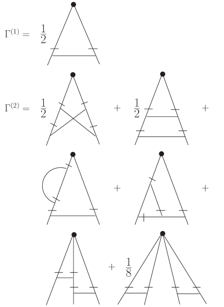
Figure 12: The Feynman diagrams for the function $\Gamma_{n,p}$ in two-loop approximation. The Feynman rules are the same as in Sec. III. The black circle is defined in the text of the present section. The one-loop diagram we denote as $K_{1}$, the two-loop diagrams we denote as $K_{2a}$ (the first diagram), $K_{2b}$ (the second diagram), $K_{2c}$ (the first diagram in the second row), $K_{2d}$ (the second diagram in the second row), $K_{2e}$ (the first diagram in the third row), and $K_{2f}$ (the second diagram in the third row).

The black circles on the top of the diagrams in Fig. 12 represents the vertex of the composite operator $F[n,p]$. Analytically it corresponds to the following expression:

$$V_{k}(x;x_{1},\ldots,x_{k})=\frac{\delta^{k}F[n,p]}{\delta\theta(x_{1})\ldots\delta\theta(x_{k})},$$ (106)

where $k$ denotes the number of attached lines. It is possible to represent it in the following convenient form (see Ref. AdAnBaKaVa01 ):

$$V(x;\,x_{1},\ldots,x_{k})=\prod_{j=1}^{k}\partial_{i_{j}}\delta(x-x_{j})\frac{\partial^{k}F[n,p]}{\partial a_{i_{1}}\ldots\partial a_{i_{k}}},$$ (107)

where $a_{i}$ is replaced by $\partial_{i}\theta(x)$ after the differentiation.

For example, the one-loop diagram shown in Fig. 12 has then the following analytical form:

$$K_{1} = \int dx_{1}\cdots\int dx_{4}V(x;\,x_{1},x_{2})\langle\theta(x_{1})\theta^{\prime}(x_{3})\rangle_{0}$$

$$\times \langle\theta(x_{2})\theta^{\prime}(x_{4})\rangle_{0}\langle v_{k}(x_{3})v_{l}(x_{4})\rangle_{0}\partial_{k}\theta(x_{3})\partial_{l}\theta(x_{4}),$$ (108)

and analogously one can write down all two-loop diagrams in Fig. 12.

To determine the renormalization constants $Z^{-1}_{[n,p]}$ it is enough to calculate the function $\Gamma^{\prime i_{1}\ldots i_{n}}_{n,p}(x;x_{1},\ldots,x_{n})$ with appropriate choice of its arguments $a_{i}$ since the function $\Gamma^{\prime i_{1}\ldots i_{n}}_{n,p}(x;x_{1},\ldots,x_{n})$ contains only logarithmic divergences. A sufficient choice is to replace them by the fixed point $x$, the argument of the operator $F[n,p]$. Thus the expression $a_{i_{1}}(x)\cdots a_{i_{n}}(x)$ in (105) can be taken outside the integration. As a result we come to the local composite operator $\Gamma_{n,p}(x;\theta)$:

$$\Gamma_{n,p}(x;\theta) = \frac{1}{n!}a_{i_{1}}(x)\cdots a_{i_{n}}(x)$$

$$\times \int dx_{1}\cdots\int dx_{n}\,\Gamma^{\prime i_{1}\ldots i_{n}}_{n,p}(x;x_{1},\ldots,x_{n}).$$

After integration one obtains an expression independent of coordinates. The vector indices of $\Gamma^{\prime i_{1}\ldots i_{n}}_{n,p}$ are transformed into combinations of Kronecker $\delta$ symbols and their contractions with vector symbols of the product $a_{i_{1}}(x)\cdots a_{i_{n}}(x)$ give the original composite operator $F[n,p]$. Expression (108) can then be written, up to an uv-finite part, in the form

$$K_{1}=a_{k}a_{l}\,\frac{\partial^{2}}{\partial a_{i}\partial a_{j}}F[n,p]X^{K_{1}}_{ij,\,kl},$$ (110)

with

$$X^{K_{1}}_{ij,\,kl} = \int dx_{3}\,\int dx_{4}\,\,\partial_{i}\langle\theta(x)\theta^{\prime}(x_{3})\rangle_{0}\,\partial_{j}\langle\theta(x)\theta^{\prime}(x_{4})\rangle_{0}$$ (111)

$$\times\langle v_{k}(x_{3})v_{l}(x_{4})\rangle_{0}.$$

Two-loop diagrams (Fig. 12) can be given in the same form, namely,

$$K_{2z} = a_{k_{1}}a_{k_{2}}\,\frac{\partial^{2}F[n,p]}{\partial a_{i_{1}}\partial a_{i_{2}}}X^{K_{2z}}_{i_{1}i_{2},\,k_{1}k_{2}},$$

$$K_{2e} = a_{k_{1}}a_{k_{2}}a_{k_{3}}\,\frac{\partial^{3}F[n,p]}{\partial a_{i_{1}}\partial a_{i_{2}}\partial a_{i_{3}}}X^{K_{2e}}_{i_{1}i_{2}i_{3},\,k_{1}k_{2}k_{3}},$$ (112)

$$K_{2f} = a_{k_{1}}a_{k_{2}}a_{k_{3}}a_{k_{4}}\,\frac{\partial^{4}F[n,p]}{\partial a_{i_{1}}\partial a_{i_{2}}\partial a_{i_{3}}\partial a_{i_{4}}}X^{K_{2f}}_{i_{1}i_{2}i_{3}i_{4},\,k_{1}k_{2}k_{3}k_{4}},$$

where $z=a,b,c,d$. The analytical expressions for $X^{K_{2z}}$ ($z=a,b,c,d,e,f$) can be easily written in analogy with the one-loop diagram $K_{1}$; therefore we shall not give their explicit form here. The tensors $X^{K_{2z}}$ in Eq. (112) can be decomposed into basic structures made of Kronecker $\delta$ symbols.

$$X^{K_{1}}_{i_{1}i_{2},k_{1}k_{2}} = \sum_{j=1}^{2}A^{K_{1}}_{j}T^{(j)}_{i_{1}i_{2},k_{1}k_{2}},$$ (113)

$$X^{K_{2z}}_{i_{1}i_{2},k_{1}k_{2}} = \sum_{j=1}^{2}A^{K_{2z}}_{j}T^{(j)}_{i_{1}i_{2},k_{1}k_{2}},$$ (114)

$$X^{K_{2e}}_{i_{1}i_{2}i_{3},k_{1}k_{2}k_{3}} = \sum_{j=1}^{2}A^{K_{2e}}_{j}T^{(j)}_{i_{1}i_{2}i_{3},k_{1}k_{2}k_{3}},$$ (115)

$$X^{K_{2f}}_{i_{1}i_{2}i_{3}i_{4},k_{1}k_{2}k_{3}k_{4}} = \sum_{j=1}^{3}A^{K_{2f}}_{j}T^{(j)}_{i_{1}i_{2}i_{3}i_{4},k_{1}k_{2}k_{3}k_{4}},$$ (116)

where $z=a,b,c,d$, and the tensor structures are defined as

$$T^{(1)}_{ij,kl}=\delta_{ij}\delta_{kl},\,\,\,T^{(2)}_{ij,kl}=\frac{\delta_{ik}\delta_{jl}+\delta_{il}\delta_{jk}}{2},$$ (117)

$$T^{(1)}_{ijk,lmn} = \frac{1}{9}\Big{(}\delta_{ij}(\delta_{kl}\delta_{mn}+\delta_{km}\delta_{ln}+\delta_{kn}\delta_{lm})$$ (118)

$$\hskip 14.22636pt+(j\leftrightarrow k)+(i\leftrightarrow k)\Big{)},$$

$$T^{(2)}_{ijk,lmn} = \frac{1}{6}\Big{(}\delta_{il}(\delta_{jm}\delta_{kn}+\delta_{jn}\delta_{km})$$ (119)

$$\hskip 14.22636pt+(l\leftrightarrow m)+(l\leftrightarrow n)\Big{)},$$

$$T^{(1)}_{ijkl,mnop} = \frac{1}{9}(\delta_{ij}\delta_{kl}+\delta_{ik}\delta_{jl}+\delta_{il}\delta_{jk})$$ (120)

$$\times(\delta_{mn}\delta_{op}+\delta_{mo}\delta_{np}+\delta_{mp}\delta_{on}),$$

$$T^{(2)}_{ijkl,mnop} = \frac{1}{72}$$

$$\times\,\,\,\,\,\,\,\,\,\,\,\,\,\,\,\,\,\,\,\, \Big{(}\delta_{ij}\big{(}\delta_{mn}(\delta_{ko}\delta_{lp}+\delta_{kp}\delta_{lo})+\delta_{mo}(\delta_{kn}\delta_{lp}+\delta_{kp}\delta_{ln})$$

$$+\,\,\,\,\,\,\,\,\, \delta_{mp}(\delta_{kn}\delta_{lo}+\delta_{ko}\delta_{ln})+\delta_{no}(\delta_{km}\delta_{lp}+\delta_{kp}\delta_{lm})$$

$$+\,\,\,\,\,\,\,\,\, \delta_{np}(\delta_{km}\delta_{lo}+\delta_{ko}\delta_{lm})+\delta_{op}(\delta_{km}\delta_{ln}+\delta_{kn}\delta_{lm})\big{)}$$

$$+\,\,\,\,\,\,\,\,\,\,\, (j\leftrightarrow k)+(j\leftrightarrow l)+(i\leftrightarrow k)+(i\leftrightarrow l)$$

$$+\,\,\,\,\,\,\,\,\,\,\, (i\leftrightarrow k,j\leftrightarrow l)\Big{)},$$ (121)

$$T^{(3)}_{ijkl,mnop} = \frac{1}{24}$$

$$\times\,\,\,\,\,\,\,\,\,\,\,\,\,\,\,\,\,\,\,\, \Big{(}\delta_{im}\big{(}\delta_{jn}(\delta_{ko}\delta_{lp}+\delta_{kp}\delta_{lo})+\delta_{jo}(\delta_{kn}\delta_{lp}+\delta_{kp}\delta_{ln})$$

$$+\,\,\,\,\,\,\,\,\, \delta_{jp}(\delta_{kn}\delta_{lo}+\delta_{ko}\delta_{ln})\big{)}$$ (122)

$$+\,\,\,\,\,\,\,\,\,\,\, (m\leftrightarrow n)+(m\leftrightarrow o)+(m\leftrightarrow o)+(m\leftrightarrow p)\Big{)},$$

and the scalar coefficients $A_{j}^{x}$ ($x=K_{1},K_{2a},\ldots,K_{2f}$) in Eqs. (113)-(116) are given as

$$A_{1}^{x} = \frac{(d+1)X_{1}^{x}-2X_{2}^{x}}{d(d+2)(d-1)},$$ (123)

$$A_{2}^{x} = \frac{2(-X_{1}^{x}+dX_{2}^{x})}{d(d+2)(d-1)},$$ (124)

for $x=K_{1},K_{2a},K_{2b},K_{2c},K_{2d}$. Further, for operator $K_{2e}$ we have

$$A_{1}^{K_{2e}} = \frac{9((d+1)X_{1}^{K_{2e}}-2X_{2}^{K_{2e}})}{d(d+2)(d+4)(d-1)},$$ (125)

$$A_{2}^{K_{2e}} = \frac{6(-3X_{1}^{K_{2e}}+(d+2)X_{2}^{K_{2e}})}{d(d+2)(d+4)(d-1)},$$ (126)

and for operator $K_{2f}$

$$A_{1}^{K_{2f}} = \frac{9(d+3)\left((d+5)X_{1}^{K_{2f}}-8X_{2}^{K_{2f}}\right)+72X_{3}^{K_{2}f}}{(d-1)d(d+1)(d+2)(d+4)(d+6)},$$ (127)

$$A_{2}^{K_{2f}} = -\frac{72\left((d+3)X_{1}^{K_{2f}}-(d^{2}+3d+6)X_{2}^{K_{2f}}+2(d+2)X_{3}^{K_{2f}}\right)}{(d-1)d(d+1)(d+2)(d+4)(d+6)},$$ (128)

$$A_{3}^{K_{2f}} = \frac{24\left(3X_{1}^{K_{2f}}+(d+2)\left(-6X_{2}^{K_{2f}}+(d+4)X_{3}^{K_{2f}}\right)\right)}{(d-1)d(d+1)(d+2)(d+4)(d+6)},$$ (129)

where $X_{j}^{x}$, $j=1,2,3,x=K_{1},K_{2a},\ldots,K_{2f}$ are given in Appendix D (calculations are performed in the MS scheme). Looking at expressions (165) and (179) in Appendix D one can see the explicit dependence of the diagrams $K_{2a}$ and $K_{2d}$ on the helicity parameter $\rho$. These diagrams are not present in the case of the rapid-change model at all ($u\rightarrow\infty$; see Ref. AdAnBaKaVa01 ) because they contain closed circuits of retarded propagators $\langle\theta\theta^{\prime}\rangle_{0}$ and therefore automatically vanish (for the same reason the self-energy operator $\Sigma_{\theta\theta^{\prime}}$ of the rapid-change model has only one-loop corrections AdAnBaKaVa01 ). This is one of the important reasons to study higher-loop corrections of models with finite correlation time, namely, some considerable properties cannot be studied within simple rapid-change models.

Let us briefly concentrate our attention on the comparison of the rapid-change limit of our two-loop results for composite operators with those obtained in Ref. AdAnBaKaVa01 . This comparison leads to some nontrivial results for the corresponding integrals. They are presented in Appendix C [expressions (162),(163), and (C)]. We found one misprint in Eq. (5.42) of Ref. AdAnBaKaVa01 , namely, there must be an overall factor $d^{2}-1$ in the expression for $A_{1}$.

The critical dimensions of our operators are defined by th egeneral formula given in Eq. (85). When we rewrite it in the concrete form of the operator $F_{np}\equiv F[n,p]=\partial_{i_{1}}\theta\cdots\partial_{i_{p}}\theta(\partial_{i}\theta\partial_{i}\theta)^{l}$ then we have

$$\Delta_{F_{np}}=d_{F_{np}}^{k}+\Delta_{\omega}d_{F_{np}}^{\omega}+\gamma^{*}_{F_{np}}\,.$$ (130)

Now using the canonical dimensions shown in Table 1, namely, $d^{k}_{\theta}=-1$ and $d^{\omega}_{\theta}=0$ one immediately comes to the result

$$\Delta_{F_{np}}=\gamma^{*}_{F_{np}}\,.$$ (131)

This means that the critical dimensions of our operators are equal to the corresponding anomalous dimensions at a corresponding fixed point.

The first step to determine the anomalous dimensions is to calculate the constants $Z_{np}\equiv Z_{[n,p][n,p]}$ [see Eq. (103)] in the two-loop approximation. In our case it is given as

$$Z_{np}=1+\frac{g}{\varepsilon}A_{np}+\frac{g^{2}}{\varepsilon}B_{np}+\frac{g^{2}}{\varepsilon^{2}}C_{np}\,.$$ (132)

The coefficient $C_{np}$ will not contribute into the corresponding anomalous dimension (this can be verified by direct calculation); hence we do not present its explicit form in what follows. The coefficients $A_{np}$ and $B_{np}$ are defined as

$$A_{np}=\frac{1}{2}\left(k_{1}^{(2)}A_{1}^{K_{1}}+k_{2}^{(2)}A_{2}^{K_{1}}\right)\,$$ (133)

and

$$B_{np} = k_{1}^{(2)}\left(\frac{1}{2}A_{1}^{K_{2a}}+\frac{1}{2}A_{1}^{K_{2a}}+A_{1}^{K_{2c}}+A_{1}^{K_{2d}}\right)$$ (134)

$$+ k_{2}^{(2)}\left(\frac{1}{2}A_{2}^{K_{2a}}+\frac{1}{2}A_{2}^{K_{2a}}+A_{2}^{K_{2c}}+A_{2}^{K_{2d}}\right)$$

$$+ k_{1}^{(3)}A_{1}^{K_{2e}}+k_{2}^{(3)}A_{2}^{K_{2e}}\,,$$

where $A_{x}^{y},x=\{1,2\},y=\{K_{1},K_{2z}\},z=\{a,b,c,d,e\}$ are defined in Eqs. (123)-(126) and

$$k_{1}^{(2)} = (n-p)(d+n+p-2)\,,$$ (135)

$$k_{2}^{(2)} = n(n-1)\,,$$ (136)

$$k_{1}^{(3)} = (n-2)(n-p)(d+n+p-2)\,,$$ (137)

$$k_{2}^{(3)} = n(n-1)(n-2).$$ (138)

Then the anomalous dimensions have the form

$$\gamma_{np}\equiv\gamma_{F_{np}}=-2A_{np}\,\,g-4B_{np}\,\,g^{2}\,.$$ (139)

Thus, the coefficient $A_{np}$ represents the one-loop contribution to the anomalous dimension, and the coefficient $B_{np}$ the two-loop one. The critical dimension $\Delta_{F_{np}}$ [see Eq. (131)] of the operator $F_{np}$ is obtained from (139) when it is taken at the corresponding fixed point.

VII.3 Anomalous scaling: Two-loop approximation

Our aim is the investigation of the influence of the helicity on the anomalous scaling in the most interesting situation of the degenerate fixed point, namely, the fixed point denoted as FPV in Sec.V. In this case, the dimensions $\Delta_{F_{np}}$ are represented in the following series in the only independent exponent $\varepsilon=\eta$ [it is obtained from (139) by the substitution of the corresponding fixed point for $g_{*}$]

$$\Delta_{F_{np}}=\varepsilon\Delta^{(1)}_{F_{np}}+\varepsilon^{2}\Delta^{(2)}_{F_{np}}\,.$$ (140)

The one-loop contribution has the form

$$\Delta^{(1)}_{F_{np}}=\frac{2n(n-1)-(n-p)(d+n+p-2)(d+1)}{2(d+2)(d-1)}\,,$$ (141)

which is independent of the parameter u (the ratio of the velocity correlation time and the scalar turnover time). Although the fixed point value $g_{*}$ given by Eq. (V) and the coefficient $B_{np}$ in Eq. (139) explicitly depend on the helicity parameter $\rho$, the two-loop contribution to the critical dimension $\Delta^{(2)}_{F_{np}}$ is independent of $\rho$. Thus, the result is the same as that obtained in Ref. AdAnHo02 (there is a misprint in the final explicit result but the correct formula was republished in Ref. AdAnHoKi05 ). Its explicit expression is rather large, and as it can be found elsewhere we shall not repeat it here. At first sight this result is a surprise but it can be understood in the following, rather simple, way. As we know the structure functions $S_{n}(r)$ (which are studied here) are functions of the value of the distance $r=|{\bf x}-{\bf x^{\prime}}|$. Therefore, only those phenomena will have impact on the critical dimensions that can ”change” the spatial distances. Among such phenomena belong the compressibility and anisotropy. As for helicity, it breaks the mirror symmetry but it does not disturb spatial distances. Therefore, it cannot influence the critical dimensions, i.e., it cannot change the corresponding asymptotic behavior. Thus, if our statement is right then we expect that the situation will be the same in all orders of perturbation expansion, namely, the quantities such as effective diffusivity will depend on helicity, but critical dimensions of the structure functions will not. But, of course, for now it is only a speculation and the independence of the critical dimensions of helicity is maybe only the effect of two-loop approximation. To solve this problem at least three-loop calculations are needed.

On the other hand, to study the helicity effect on the two-loop level it is enough to avoid the conditions of isotropy or incompressibility of the system. Thus, the next step is, e.g., to include the assumption of compressibility of the system and investigate the combined effects of the helicity and compressibility on the scaling properties of the model under consideration. We assume that a nontrivial result can be obtained.

As was already mentioned detailed analysis of the two-loop contribution to the critical dimensions of the structure functions within the model under our consideration (without helicity) was done in Ref. AdAnHo02 . We have recalculated their results and found some discrepancy in interpretations of our and their numerical results. That is, as our calculations show, a hierarchical behavior of the quantity $\zeta_{n}\equiv\left[\Delta_{n0}^{(2)}-\Delta_{n0}^{(2)}|_{u=\infty}\right]/n^{3}$ as a function of $n$ for a concrete value of $d$ (dimension of space) is destroyed in Fig. 1(d) in Ref. AdAnHo02 . This figure corresponds to a large enough value of $d$ (namely, $d=10$). Our calculations lead to the same curves as theirs but they correspond to different values of $n$ which can be seen by direct comparison of Fig. 1(d) in Ref. AdAnHo02 and Fig. 13 in the present paper.

Figure 13: Behavior of the quantity $\zeta_{n}$ (see text) for $n=4,6,8,10,20,$ and $50$ as a function of $u$ for $d=10$ in units of $10^{-3}$. In Ref. AdAnHo02 the curves are interpreted as $n=4,6,8,20$ (from bottom to top). But in fact they correspond to $n=20,4,8,6$ (from bottom to top). The curves for $n=10,50$ are added to demonstrate the situation more completely.

The conclusion is as follows: The hierarchical behavior of the quantities $\zeta_{n}$ is not present for large enough space dimensions $d$ (the same situation also occurs for other large values of $d$ as can be shown by direct calculations).

All the other results are the same as in Ref. AdAnHo02 ; thus we shall not repeat them here.

VIII Conclusion

In this paper, the influence of helicity on the stability of asymptotic regimes, on the anomalous scaling, and on the effective diffusivity was studied in the framework of the passive scalar advected by the turbulent flow with finite correlations in time of the velocity field. Such investigation is important and useful for understanding of efficiency of toy models (like the Kraichnan and related model) to study the real turbulent motions by means of modern theoretical methods including renormalization group approach. Thus, it can be considered as the first step in investigation of the influence of helicity in a real turbulent environment.

In the present paper, the RG calculations are performed in the two-loop approximation, which is necessary to include the effects of helicity. It was shown that the anomalous scaling of the structure functions, which is typical for the Kraichnan model and its numerous extensions (see the Introduction), is not changed by the inclusion of helicity in the incompressible fluid. This is given mathematically by the very interesting fact that although separated two-loop Feynman diagrams of the corresponding composite operators strongly depend on the helicity parameter $\rho$, their sum - the critical dimension $\Delta_{n}$ - is independent of $\rho$ in the asymptotic regime defined by an ir stable fixed point. This very interesting fact can be explained physically by rather simple arguments in the following way (as was discussed in the previous section maybe it is only the effect of the two-loop approximation, therefore, to confirm what follows higher-loop calculations are needed). The single-time structure functions $S_{n}(r)$ of the scalar field depend only on the spatial distance $r=|{\bf x}-{\bf x^{\prime}}|$ but not on the direction. Thus, we suppose that only this phenomenon will change the critical dimensions of structure functions which modify spatial relations. It can be, e.g., the inclusion of compressibility or spatial anisotropy. On the other hand, helicity breaks the mirror symmetry, which is not related to distance. As a result, the critical dimensions of the structure functions are not affected by the helicity of the system. We suppose that an analogous situation will hold for all quantities that depend only on the spatial distance (more precisely, that are constructed from quantities taken at different spatial points), and in all orders of perturbation theory. The situation can be different when one includes in the investigation the effects of helicity together with another assumption about the turbulent flow, e.g., its compressibility. We suppose that nontrivial results can be obtained in this more general case.

On the other hand, the stability of possible asymptotic regimes, the values of the fixed RG points, and the turbulent diffusivity strongly depend on the amount of helicity. It is shown that the presence of helicity in the system leads to restrictions on the possible values of the parameters of the model. The most interesting fact is the existence of a critical value $\rho_{c}$ of the helicity parameter $\rho$ which divides the interval of possible absolute values of $\rho$ into two parts with completely different behavior. It is related to the existence of a competition between nonhelical and helical contributions within the two-loop approximation. As a result of this competition, within the so-called frozen limit, the presence of helicity enlarges the region of parameter space with a stable scaling regime, and if $|\rho|=\rho_{c}$ the corresponding two-loop restriction vanishes completely and one comes to the one-loop results Antonov99 . Similar splitting, although more complicated, into two nontrivial behaviors of the fixed point was also obtained in the general case with finite correlations in time of the velocity field.

Another quantity which rather strongly depends on the helicity parameter $\rho$ is the effective diffusivity. It is shown that the value of effective diffusivity can be 50% larger in the helical case in comparison with the nonhelical case.

Appendix A

In principle a few ways exist to evaluate the two-loop diagrams $B_{1}$ and $B_{2}$ which are explicitly shown in Fig. 3. We compare two of them on the example of the Feynman diagram $B_{1}$. The explicit analytical expression for $B_{1}$ in the wave-number-frequency representation is

$$B_{1} = \frac{g^{2}\nu^{6}\mu^{4\varepsilon}}{(2\pi)^{2d+2}}\int\frac{d^{d}{\bf k}d^{d}{\bf q}d\omega_{k}d\omega_{q}k^{4-d-2\varepsilon}q^{4-d-2\varepsilon}}{(\omega^{2}_{k}+\nu^{2}u^{2}k^{4})(\omega^{2}_{q}+\nu^{2}u^{2}q^{4})}$$ (142)

$$\times\frac{p_{i_{1}}(p-k)_{i_{3}}(p-k-q)_{i_{4}}(p-k)_{i_{2}}P^{\rho}_{i_{1}i_{2}}(k)P^{\rho}_{i_{3}i_{4}}(q)}{(i\omega_{k}+\nu({\bf p}-{\bf k})^{2})^{2}(i(\omega_{k}+\omega_{q})+\nu({\bf p}-{\bf k}-{\bf q})^{2})},$$

where ${\bf p}$ denotes the external wave number (momentum), ${\bf k}$ and ${\bf q}$ are two independent internal wave numbers, the external frequency $\omega_{p}$ is taken to be zero (we are only interested in the divergent part of the diagram and it is independent of $\omega_{p}$), $\omega_{k}$ and $\omega_{q}$ are the corresponding internal frequencies, $\eta$ is taken to be zero (see discussion in Sec. IV), $P^{\rho}_{ij}$ is the helical transverse projector defined in Sec. II, and over the internal vector indices $i_{j},j=1,2,3,4$, corresponding summations are assumed.

After integration over the internal frequencies, which is rather simple, and then making an expansion in respect of the external momentum ${\bf p}$ and leaving only terms of order two in respect of ${\bf p}$ (because uv divergences can have only this structure; see Sec. IV), and, in the end, after summation over vector indices one has

$$B_{1} = \frac{g^{2}\nu\mu^{4\varepsilon}}{(2\pi)^{2d}4u^{2}(1+u)^{2}}\int\frac{d^{d}{\bf k}d^{d}{\bf q}k^{-d-2\varepsilon}q^{-d-2\varepsilon}}{((1+u)(k^{2}+q^{2})+2{\bf k}\cdot{\bf q})}$$ (143)

$$\times\Bigg{[}p^{2}q^{2}-\frac{({\bf p}\cdot{\bf k})^{2}q^{2}}{k^{2}}-\frac{p^{2}({\bf k}\cdot{\bf q})^{2}}{k^{2}}+\frac{({\bf p}\cdot{\bf k})^{2}({\bf k}\cdot{\bf q})^{2}}{k^{4}}\Bigg{]}.$$

Now we shall calculate $B_{1}$ in two different ways.

The first approach to the integral $B_{1}$ is based on division of integrations into radial and angle parts which after standard procedures leads to (for details see, e.g., Ref. AdAnBaKaVa01 )

$$B_{1} = \frac{g^{2}\nu\mu^{4\varepsilon}p^{2}S_{d}S_{d-1}}{(2\pi)^{2d}4u^{2}(1+u)^{2}}\frac{d-1}{d}$$

$$\times\int_{m}^{\infty}\frac{dk}{k^{1+2\varepsilon}}\int_{m}^{\infty}\frac{dq}{q^{1+2\varepsilon}}\int_{-1}^{1}dx\frac{(1-x^{2})^{(d-1)/2}q^{2}}{(1+u)(k^{2}+q^{2})+2kqx},$$

where $x=\cos\psi$, and $\psi$ denotes the angle between vectors ${\bf k}$ and ${\bf q}$. $S_{d}$ and $S_{d-1}$ are $d$-dimensional and $(d-1)$-dimensional sphere, respectively, which are defined as $S_{d}=2\pi^{d/2}/\Gamma(d/2)$. The needed ir cutoff of the integrations is represented by $m\sim L^{-1}$. It is useful to rewrite the denominator of the expression under the integration in the form of the infinite series

$$\frac{1}{(1+u)(k^{2}+q^{2})+2kqx}=\sum_{j=1}^{\infty}\frac{(-2kqx)^{j-1}}{[(k^{2}+q^{2})(1+u)]^{j}}$$ (145)

Now we are able to integrate over the angle variable $x=\cos\psi$ term by term in the sum, which yields

$$B_{1} = \frac{g^{2}\nu\mu^{4\varepsilon}p^{2}S_{d}S_{d-1}}{(2\pi)^{2d}8u^{2}(1+u)^{2}}\frac{d-1}{d}\Gamma\left(\frac{d+1}{2}\right)$$ (146)

$$\sum_{j=1}^{\infty}((-1)^{j-1}+1)\frac{\Gamma\left(\frac{j}{2}\right)}{\Gamma\left(\frac{d+j+1}{2}\right)}$$

$$\int_{m}^{\infty}\frac{dk}{k^{1+2\varepsilon}}\int_{m}^{\infty}\frac{dq}{q^{1+2\varepsilon}}\frac{q^{2}(2kq)^{j-1}}{[(k^{2}+q^{2})(1+u)]^{j}}.$$

The factor $[(-1)^{j-1}+1]$ keeps only odd terms of the series. Therefore, we can redefine the summation in Eq. (146) in the following form:

$$B_{1} = \frac{g^{2}\nu\mu^{4\varepsilon}p^{2}S_{d}S_{d-1}(d-1)\Gamma\left(\frac{d+1}{2}\right)}{(2\pi)^{2d}4u^{2}(1+u)^{2}d}\sum_{j=0}^{\infty}\frac{\Gamma\left(\frac{2j+1}{2}\right)}{\Gamma\left(\frac{d+2j+2}{2}\right)}$$ (147)

$$\int_{m}^{\infty}\frac{dk}{k^{1+2\varepsilon}}\int_{m}^{\infty}\frac{dq}{q^{1+2\varepsilon}}\frac{q^{2}(2kq)^{2j}}{[(k^{2}+q^{2})(1+u)]^{2j+1}}.$$

To proceed it is appropriate to make transformation of the variables $k,q$ to the new polar coordinates, namely: $k=s\cos\phi,q=s\sin\phi$. This gives

$$B_{1} = \frac{g^{2}\nu\mu^{4\varepsilon}p^{2}S_{d}S_{d-1}(d-1)\Gamma\left(\frac{d+1}{2}\right)}{(2\pi)^{2d}4u^{2}(1+u)^{2}d}$$ (148)

$$\sum_{j=0}^{\infty}\frac{\Gamma\left(\frac{2j+1}{2}\right)}{\Gamma\left(\frac{d+2j+2}{2}\right)}\frac{2^{2j}}{(1+u)^{2j+1}}\int_{m}^{\infty}\frac{ds}{s^{1+4\varepsilon}}$$

$$\int_{0}^{\pi/2}d\phi\cos\phi^{2j-1-2\varepsilon}\sin\phi^{2j+1-2\varepsilon}.$$

The integral over the radial variable $s$ is trivial, and the integral over angle $\phi$ can be found, e.g., in Ref. GradRizi . Then one has

$$B_{1} = \frac{g^{2}\nu p^{2}\pi^{1/2}S_{d}S_{d-1}(d-1)\Gamma\left(\frac{d+1}{2}\right)}{(2\pi)^{2d}32u^{2}(1+u)^{2}d}\left(\frac{\mu}{m}\right)^{4\varepsilon}\frac{1}{\varepsilon}$$ (149)

$$\sum_{j=0}^{\infty}\frac{\Gamma\left(\frac{2j+1}{2}\right)}{\Gamma\left(\frac{d+2j+2}{2}\right)}\frac{2^{2\varepsilon}}{(1+u)^{2j+1}}\frac{\Gamma\left(j-\varepsilon\right)}{\Gamma\left(\frac{1}{2}+j-\varepsilon\right)}.$$

In the end, the summation over $j$ leads to the final result for $B_{1}$ which is given in Eq. (IV), where only the divergent part is shown. $\Gamma\left(j-\varepsilon\right)$ in Eq. (149) for $j=0$ has a pole with respect to $\varepsilon$, which gives the pole of the second order in $B_{1}$ in Eq. (IV).

The second approach to the calculation of our two-loop diagrams is as follows. We start with the expression for $B_{1}$ as represented in Eq. (143). Now using the well-known formula of Feynman parametrization

$$\frac{1}{A_{1}^{\alpha_{1}}A_{2}^{\alpha_{2}}\cdots A_{n}^{\alpha_{n}}} = \frac{\Gamma\Big{(}\sum\limits_{i=1}^{n}\alpha_{i}\Big{)}}{\prod\limits_{i=1}^{n}\Gamma\left(\alpha_{i}\right)}$$ (150)

$$\times\int_{0}^{1}\cdots\int_{0}^{1}du_{1}\cdots du_{n}\frac{\delta\Big{(}\sum\limits_{i=1}^{n}\alpha_{i}-1\Big{)}\prod\limits_{i=1}^{n}u_{i}^{\alpha_{i}-1}}{\Big{(}\sum\limits_{i=1}^{n}A_{i}u_{i}\Big{)}^{\sum\limits_{i=1}^{n}\alpha_{i}}}$$

$B_{1}$ obtains the form

$$B_{1} = \frac{g^{2}\nu\mu^{4\varepsilon}\Big{(}\frac{d}{2}+\varepsilon\Big{)}}{(2\pi)^{2d}4u^{2}(1+u)^{2}}\int_{0}^{1}du_{1}u_{1}^{\frac{d}{2}+\varepsilon-1}$$ (151)

$$\int\frac{d{\bf k}d{\bf q}\left(p^{2}-\frac{({\bf p}\cdot{\bf k})^{2}}{k^{2}}\right)\left(q^{2}-\frac{({\bf k}\cdot{\bf q})^{2}}{k^{2}}\right)}{k^{d+2\varepsilon}[Xq^{2}+2Y{\bf k}\cdot{\bf q}+Zk^{2}]^{\frac{d}{2}+\varepsilon+1}},$$

where

$$X = u_{1}+(1-u_{1})(1+u),$$

$$Y = 1-u_{1},$$ (152)

$$Z = (1+u)(1-u_{1}).$$

The integration over ${\bf q}$ is now done using the general formula (157) given in Appendix B, namely,

$$\int d{\bf q}\frac{q_{i}q_{j}}{[Xq^{2}+2Y{\bf k}\cdot{\bf q}+Zk^{2}]^{\frac{d}{2}+\varepsilon+1}} = \frac{\pi^{\frac{d}{2}}X^{-1-\frac{d}{2}}}{\Gamma\left(\frac{d}{2}+\varepsilon+1\right)}$$ (153)

$$\frac{1}{k^{2\varepsilon}\left(Z-\frac{Y^{2}}{X}\right)^{\varepsilon}}\left[\Gamma(\varepsilon)\frac{\delta_{ij}}{2}+\frac{\Gamma(\varepsilon+1)Y^{2}}{\left(XZ-Y^{2}\right)}\frac{k_{i}k_{j}}{k^{2}}\right],$$

which yields

$$B_{1} = \frac{g^{2}\nu\mu^{4\varepsilon}\pi^{\frac{d}{2}}(d-1)}{(2\pi)^{2d}8u^{2}(1+u)^{2}}\frac{\Gamma\left(\varepsilon\right)}{\Gamma\left(\frac{d}{2}+\varepsilon\right)}$$ (154)

$$\int_{0}^{1}du_{1}\frac{u_{1}^{\frac{d}{2}+\varepsilon-1}X^{-\frac{d}{2}-1}}{\left(Z-\frac{Y^{2}}{X}\right)^{\varepsilon}}\int d{\bf k}\frac{\left(p^{2}-\frac{{\bf p}\cdot{\bf k}}{k^{2}}\right)}{k^{d+4\varepsilon}}.$$

The integration over vector ${\bf k}$ is now straightforward, after which we have

$$B_{1} = \frac{g^{2}\nu S_{d}\pi^{\frac{d}{2}}p^{2}(d-1)^{2}}{(2\pi)^{2d}32u^{2}(1+u)^{2}d\Gamma\left(\frac{d}{2}+\varepsilon\right)}\left(\frac{\mu}{m}\right)^{4\varepsilon}\frac{\Gamma(\varepsilon)}{\varepsilon}$$ (155)

$$\int_{0}^{1}du_{1}\frac{u_{1}^{\frac{d}{2}+\varepsilon-1}X^{-\frac{d}{2}-1}}{\left(Z-\frac{Y^{2}}{X}\right)^{\varepsilon}}\,,$$

where $m\sim L^{-1}$ represents the needed ir regularization. We are interested only in the divergent (poles in $\varepsilon$) part of the expression (155). After doing all needed expansions with respect to $\varepsilon$ one has the final result for the Feynman diagram $B_{1}$:

$$B_{1} = \frac{S_{d}^{2}p^{2}g^{2}\nu(d-1)^{2}}{(2\pi)^{2d}32u^{2}(1+u)^{3}d^{2}}\left(\frac{\mu}{m}\right)^{4\varepsilon}\bigg{\{}\frac{1}{\varepsilon^{2}}$$ (156)

$$+\frac{1}{\varepsilon}\bigg{[}\psi(1)-\psi\left(d/2\right)-\frac{2}{d(1+u)^{\frac{d}{2}}}{{}_{2}F_{1}}\Big{(}\frac{d}{2},\frac{d}{2};1+\frac{d}{2};\frac{u}{1+u}\Big{)}$$

$$-\frac{d(1+u)}{2}\int_{0}^{1}du_{1}\frac{u_{1}^{\frac{d}{2}-1}\ln\left(Z-\frac{Y^{2}}{X}\right)}{X^{\frac{d}{2}+1}}\bigg{]}\bigg{\}},$$

where $\psi(n)$ is the logarithmic derivative of the gamma function, given by $\psi(n)=\Gamma^{\prime}(n)/\Gamma(n)$.

Thus, we have two different analytical representations of the same Feynman diagram $B_{1}$, namely, Eqs. (IV) and (156). The comparison of them leads to the nontrivial result for integral in Eq. (156), which is present in Appendix C in Eq. (159). The comparison of the results for diagram $B_{2}$ (see Fig. 3) obtained by these two methods yields other nontrivial results for some integrals. They are shown in Appendix C in Eqs. (160) and (161).

Appendix B

In this appendix we introduce the general integral formula which was used in the previous appendix.

Theorem: Let $\mathcal{V}$ be a $d$-dimensional Euclidean vector space over the field of real numbers $\mathbb{R}$. Let $l,n\in\mathbb{N}$ (natural numbers), and ${\bf k}^{(i)}$ for $i=1,2,\cdots,l$ are vectors in $\mathcal{V}$. Then for an arbitrary $l\times l$ real matrix $v_{js}$ with $\det v\neq 0$, arbitrary vectors ${\bf a}^{(i)}$ ($i=1,2,\cdots,l$), and arbitrary $c,\alpha\in\mathbb{R}$ the following general formula holds:

$$\int^{\infty}_{-\infty} \ldots\int^{\infty}_{-\infty}\frac{d{\bf k}^{(1)}\ldots d{\bf k}^{(l)}k_{i_{1}}^{(q_{1})}k_{i_{2}}^{(q_{2})}\ldots k_{i_{n}}^{(q_{n})}}{\left[v_{is}{\bf k}^{(i)}\cdot{\bf k}^{(s)}+2{\bf a}^{(i)}\cdot{\bf k}^{(i)}+c\right]^{\alpha}}=$$ (157)

$$\frac{(-1)^{n}\pi^{\frac{dl}{2}}(\mathrm{det}\;v)^{-\frac{d}{2}}}{\Gamma(\alpha)}\;\sum_{p=0}^{\lfloor\frac{n}{2}\rfloor}\;\frac{\Gamma\left(\alpha-\frac{dl}{2}-\lfloor\frac{n}{2}\rfloor+p\right)\left[c-(v^{-1})_{is}{\bf a}^{(i)}\cdot{\bf a}^{(s)}\right]^{\lfloor\frac{n}{2}\rfloor+\frac{dl}{2}-\alpha-p}}{(\lfloor\frac{n}{2}\rfloor-p)!\,(2p+n(\mathrm{mod}\;2))!4^{\lfloor\frac{n}{2}\rfloor-p}}$$

$$\sum_{P(q_{1}i_{1},q_{2}i_{2},\ldots,q_{n}i_{n})}(v^{-1})_{q_{1}s_{1}}a_{i_{1}}^{(s_{1})}(v^{-1})_{q_{2}s_{2}}a_{i_{2}}^{(s_{2})}\ldots(v^{-1})_{q_{2p+n(\mathrm{mod}\;2)}s_{2p+n(\mathrm{mod}\;2)}}a_{i_{2p+n(\mathrm{mod}\;2)}}^{(s_{i_{2p+n(\mathrm{mod}\;2)}})}$$

$$\times \delta_{i_{2p+n(\mathrm{mod}\;2)+1}i_{2p+n(\mathrm{mod}\;2)+2}}(v^{-1})_{q_{2p+n(\mathrm{mod}\;2)+1}q_{2p+n(\mathrm{mod}\;2)+2}}\ldots\delta_{i_{n-1}i_{n}}(v^{-1})_{q_{n-1}q_{n}},$$

where the summation is taken over all permutations of the indices $i_{1},i_{2},\ldots,i_{n}$, $k_{j}^{(s)}$ and $a_{j}^{(s)}$ are the $j$th components of the vectors ${\bf k}^{(s)}$ and ${\bf a}^{(s)}$, $\delta_{ij}$ denotes the Kronecker delta, and $\lfloor n/2\rfloor=n/2$ for even $n$ and $\lfloor n/2\rfloor=(n-1)/2$ for odd $n$. Over all dummy indices the corresponding summation is assumed.

We shall not present a detailed proof here because it is rather large although straightforward; instead we give a short recipe for it. To prove formula (157) it is appropriate to use mathematical induction. First, the theorem is correct in the scalar case ($n=0$). In this specific situation the formula is well known (see, e.g., Ref. Vasiliev )

$$\int^{\infty}_{-\infty}\ldots\int^{\infty}_{-\infty}\frac{d{\bf k}^{(1)}\ldots d{\bf k}^{(l)}}{\left[v_{is}{\bf k}^{(i)}\cdot{\bf k}^{(s)}+2{\bf a}^{(i)}\cdot{\bf k}^{(i)}+c\right]^{\alpha}} =$$ (158)

$$\frac{\pi^{\frac{dl}{2}}(\mathrm{det}v)^{-\frac{d}{2}}\Gamma\left(\alpha-\frac{dl}{2}\right)}{\Gamma(\alpha)}\left[c-(v^{-1})_{is}{\bf a}^{(i)}\cdot{\bf a}^{(s)}\right]^{\frac{dl}{2}-\alpha}.$$

Now, let us suppose that formula (157) is valid for $n\in\mathbb{N},\;n\geq 1$. Then if one differentiates both sides of Eq. (157) with respect to $a^{(q_{n+1})}_{i_{n+1}}$ together with some cumbersome algebraic manipulations the formula for $n+1$ is obtained.

Appendix C

In this appendix we present the integrals that were obtained during the calculations of two-loop Feynman diagrams $B_{1}$ and $B_{2}$ which are shown in Fig. 3 (see Appendix A for details of the calculations). They are given in Eqs. (159)-(161). In addition we present here the analytical expressions for integrals that were obtained by comparison of our two-loop results for composite operators with those obtained within the rapid-change model AdAnBaKaVa01 [Eqs. (162)-(C)].

$$\int_{0}^{1}\,du_{1}\frac{u_{1}^{\frac{d}{2}-1}\ln\left((1+u)(1-u_{1})-\frac{(1-u_{1})^{2}}{u_{1}+(1+u)(1-u_{1})}\right)}{\left[u_{1}+(1+u)(1-u_{1})\right]^{\frac{d}{2}+1}} =$$ (159)

$$\frac{4}{d(1+u)}\bigg{\{}\frac{\psi(1)-\psi\left(d/2\right)}{2}-\frac{{{}_{2}F_{1}}\Big{(}\frac{d}{2},\frac{d}{2};1+\frac{d}{2};\frac{u}{1+u}\Big{)}}{d(1+u)^{\frac{d}{2}}}$$

$$-\frac{{{}_{2}F_{1}}\Big{(}1,1;2+\frac{d}{2};\frac{1}{(1+u)^{2}}\Big{)}}{(d+2)(1+u)^{2}}\bigg{\}},$$

$$\int_{0}^{1}\,du_{1}\frac{u_{1}^{\frac{d}{2}}(1+u(1-u_{1}))^{-\frac{d}{2}-1}}{\left[u(2+u)-u_{1}(u^{2}+u-1)\right]} =$$ (160)

$$\frac{2}{(d+2)(1+u)^{2}}\,{{}_{2}F_{1}}\Big{(}1,1;2+\frac{d}{2};\frac{1}{(1+u)^{2}}\Big{)},$$

$$\int_{0}^{1}du_{1}\frac{u_{1}[(u_{1}+(1+u)(1-u_{1}))(1+u)-(1-u_{1})]^{-\frac{1}{2}}}{(u_{1}+(1+u)(1-u_{1}))^{2}(1-u_{1})^{\frac{1}{2}}}$$ (161)

$$=\frac{4}{3(1+u)}{{}_{2}F_{1}}\Big{(}\frac{1}{2},\frac{1}{2};\frac{5}{2};\frac{1}{(1+u)^{2}}\Big{)},$$

$$\int_{-1}^{1}dx\,\,(1-x^{2})^{d/2}\,x\,\arctan\left(\frac{1+x}{\sqrt{1-x^{2}}}\right)$$ (162)

$$=\frac{1}{2}\frac{S_{d}}{S_{d-1}}\frac{d^{2}-1}{d(d+2)^{2}}\,,$$

$$\int_{-1}^{1}dx\,\,\frac{(1-x^{2})^{(d+1)/2}\,x}{\sqrt{4-x^{2}}}\,\arctan\left(\frac{2+x}{\sqrt{4-x^{2}}}\right)$$ (163)

$$=\frac{1}{8}\frac{S_{d}}{S_{d-1}}\frac{d^{2}-1}{d(d+2)(d+4)}{{}_{2}F_{1}}\Big{(}1,1;3+\frac{d}{2};\frac{1}{4}\Big{)}\,,$$

$$\int_{-1}^{1}dx\,\,\frac{(1-x^{2})^{(d+1)/2}\,x^{3}}{\sqrt{4-x^{2}}}\,\arctan\left(\frac{2+x}{\sqrt{4-x^{2}}}\right)$$

$$=\frac{1}{8}\frac{S_{d}}{S_{d-1}}\frac{d^{2}-1}{d(d+2)(d+4)}$$

$$\times\Biggl{[}{{}_{2}F_{1}}\Big{(}1,1;3+\frac{d}{2};\frac{1}{4}\Big{)}-\frac{d+3}{d+6}\,\,{{}_{2}F_{1}}\Big{(}1,1;4+\frac{d}{2};\frac{1}{4}\Big{)}\Biggr{]}\,,$$

Appendix D

The explicit form of the coefficients $X_{j}^{x}$, $j=1,2,3,x=K_{1},K_{2a},\ldots,K_{2f}$ (see Sec.VII), in the MS scheme is the following:

$$X^{K_{1}}_{1}=\frac{S_{d}}{(2\pi)^{d}}\left(\frac{\mu}{m}\right)^{2\varepsilon}\frac{d-1}{4u(1+u)}\frac{g}{\varepsilon}\,,\,\,\,\,\,X^{K_{1}}_{2}=0\,,$$ (164)

$$X^{K_{2a}}_{1} = \frac{g^{2}S_{d}^{2}}{(2\pi)^{2d}16u^{2}(1+u)(1-u^{2})}\frac{d-1}{d}\frac{1}{\varepsilon}\left(\frac{\mu}{m}\right)^{4\varepsilon}\Bigg{[}\frac{{{}_{2}F_{1}}\left(1,1;2+\frac{d}{2};\frac{1}{(1+u)^{2}}\right)-u\,\,{{}_{2}F_{1}}\left(1,1;2+\frac{d}{2};\frac{1}{2(1+u)}\right)}{(d+2)(1+u)}$$ (165)

$$+\,\,\pi\rho^{2}(d-2)\left(-\frac{1}{2}\,\,{{}_{2}F_{1}}\left(\frac{1}{2},\frac{1}{2};1+\frac{d}{2};\frac{1}{(1+u)^{2}}\right)+\frac{u}{\sqrt{2(1+u)}}\,\,{{}_{2}F_{1}}\left(\frac{1}{2},\frac{1}{2};1+\frac{d}{2};\frac{1}{2(1+u)}\right)\right)\Bigg{]}\,,$$

$$X^{K_{2a}}_{2}=X^{K_{2a}}_{2a}+X^{K_{2a}}_{2b}\,,$$ (166)

$$X^{K_{2a}}_{2a} = \frac{g^{2}S_{d}^{2}}{(2\pi)^{2d}32u^{3}(1+u)(1-u^{2})}\frac{(d-1)(d+1)}{d(d+2)}\frac{1}{\varepsilon}\left(\frac{\mu}{m}\right)^{4\varepsilon}$$ (167)

$$\times\left[(1+u)\,\,{{}_{3}F_{2}}\left(\frac{1}{2},1,1;\frac{3}{2},2+\frac{d}{2};1\right)-{{}_{3}F_{2}}\left(\frac{1}{2},1,1;\frac{3}{2},2+\frac{d}{2};\frac{1}{(1+u)^{2}}\right)\right]\,,$$

$$X^{K_{2a}}_{2b} = \frac{g^{2}S_{d}S_{d-1}}{(2\pi)^{2d}16u(1+u)(1-u^{2})}\frac{1}{\varepsilon}\left(\frac{\mu}{m}\right)^{4\varepsilon}\int^{1}_{-1}dx\,\frac{(1-x^{2})^{\frac{d+1}{2}}}{(1-u)^{2}+4ux^{2}}$$ (168)

$$\left(-\frac{2(1+u)x\arctan\left(\frac{x}{\sqrt{1-x^{2}}}\right)}{\sqrt{1-x^{2}}}+\frac{2(1+3u)x\arctan\left(\frac{x}{\sqrt{2(1+u)-x^{2}}}\right)}{\sqrt{2(1+u)-x^{2}}}+(u-1)\ln\left(\frac{2}{1+u}\right)\right)\,,$$

$$X^{K_{2b}}_{1}=X^{K_{2b}}_{1a}+X^{K_{2b}}_{1b}\,,$$ (169)

$$X^{K_{2b}}_{1a}=\frac{g^{2}S_{d}^{2}}{(2\pi)^{2d}32u^{2}(1+u)^{2}}\frac{(d-1)^{2}}{d}\left(\frac{\mu}{m}\right)^{4\varepsilon}\frac{1}{\varepsilon}\left(\frac{1}{\varepsilon}+\frac{2\,\,{{}_{2}F_{1}}\left(1,1;2+\frac{d}{2};\frac{1}{(1+u)^{2}}\right)}{(d+2)(1+u)^{2}(1-u)}-\frac{u\ln\left(\frac{1+u}{2}\right)}{(1-u)}\right)\,,$$ (170)

$$X^{K_{2b}}_{1b} = -\frac{g^{2}S_{d}S_{d-1}(d-1)}{(2\pi)^{2d}16u(1+u)(1-u^{2})}\left(\frac{\mu}{m}\right)^{4\varepsilon}\frac{1}{\varepsilon}$$ (171)

$$\times\int_{-1}^{1}dx\,(1-x^{2})^{\frac{d-1}{2}}x\,\,\frac{\arctan\left(\frac{2+x}{\sqrt{2(1+u)-x^{2}}}\right)+\arctan\left(\frac{1+u+x}{\sqrt{2(1+u)-x^{2}}}\right)}{\sqrt{2(1+u)-x^{2}}}\,,$$

$$X^{K_{2b}}_{2}=X^{K_{2b}}_{2a}+X^{K_{2b}}_{2b}\,,$$ (172)

$$X^{K_{2b}}_{2a} = \frac{g^{2}S_{d}^{2}}{(2\pi)^{2d}32u^{2}(1+u)(1-u^{2})}\frac{d^{2}-1}{d(d+2)}\left(\frac{\mu}{m}\right)^{4\varepsilon}\frac{1}{\varepsilon}\Biggl{\{}\frac{1-u}{\varepsilon}-1+\frac{4}{15(4+d)(6+d)u(1+u)^{4}}$$ (173)

$$\times\Biggl{[}5(6+d)(1+u)^{2}\left((1+u)^{3}\,\,{{}_{3}F_{2}}\left(1,1,\frac{3}{2};\frac{5}{2},3+\frac{d}{2};1\right)-{{}_{3}F_{2}}\left(1,1,\frac{3}{2};\frac{5}{2},3+\frac{d}{2};\frac{1}{(1+u)^{2}}\right)\right)$$

$$\hskip 14.22636pt+\left((1+u)^{5}\,\,{{}_{3}F_{2}}\left(2,2,\frac{5}{2};\frac{7}{2},4+\frac{d}{2};1\right)-{{}_{3}F_{2}}\left(2,2,\frac{5}{2};\frac{7}{2},4+\frac{d}{2};\frac{1}{(1+u)^{2}}\right)\right)\Biggr{]}\Biggr{\}}\,,$$

$$X^{K_{2b}}_{2b} = -\frac{g^{2}S_{d}S_{d-1}}{(2\pi)^{2d}16u(1+u)(1-u^{2})}\left(\frac{\mu}{m}\right)^{4\varepsilon}\frac{1}{\varepsilon}\int_{-1}^{1}dx\,\frac{(1-x^{2})^{\frac{d+1}{2}}}{(1-u)^{2}+4ux^{2}}\Biggl{[}(u-1+2x^{2})\ln\left(\frac{2}{1+u}\right)$$

$$+2x\left(\frac{(1+u)(u-3+4x^{2})\arctan\left(\frac{1+x}{\sqrt{1-x^{2}}}\right)}{\sqrt{1-x^{2}}}+\frac{(3+u-2x^{2})\left(\arctan\left(\frac{2+x}{\sqrt{2(1+u)-x^{2}}}\right)+\arctan\left(\frac{1+u+x}{\sqrt{2(1+u)-x^{2}}}\right)\right)}{\sqrt{2(1+u)-x^{2}}}\right)\Biggr{]}\,,$$

$$X^{K_{2c}}_{1} = X^{K_{2c}}_{1a}+X^{K_{2c}}_{1b}\,,$$ (175)

$$X^{K_{2c}}_{1a} = -\frac{1}{1+u}X^{K_{2b}}_{1a}\,,$$ (176)

$$X^{K_{2c}}_{1b} = -\frac{1}{2}X^{K_{2b}}_{1b}\,,$$ (177)

$$X^{K_{2c}}_{2} = 0\,,$$ (178)

$$X^{K_{2d}}_{1} = -\frac{g^{2}S_{d}^{2}}{(2\pi)^{2d}16u^{2}(1+u)(1-u^{2})}\frac{d-1}{d}\left(\frac{\mu}{m}\right)^{4\varepsilon}\frac{1}{\varepsilon}$$ (179)

$$\times\Biggl{\{}\frac{1}{(2+d)(1+u)}\left[\frac{{{}_{2}F_{1}}\left(1,1;2+\frac{d}{2};\frac{1}{(1+u)^{2}}\right)}{1+u}-\frac{u\,\,{{}_{2}F_{1}}\left(1,1;2+\frac{d}{2};\frac{1}{2(1+u)}\right)}{2}\right]$$

$$\hskip 14.22636pt+\frac{(d-2)\pi\rho^{2}}{2}\left[-\frac{{{}_{2}F_{1}}\left(\frac{1}{2},\frac{1}{2};1+\frac{d}{2};\frac{1}{(1+u)^{2}}\right)}{1+u}+\frac{u\,\,{{}_{2}F_{1}}\left(\frac{1}{2},\frac{1}{2};1+\frac{d}{2};\frac{1}{2(1+u)}\right)}{\sqrt{2(1+u)}}\right]\Biggr{\}}\,,$$

$$X^{K_{2d}}_{2} = 0\,,$$ (180)

$$X^{K_{2e}}_{1}=X^{K_{2e}}_{1a}+X^{K_{2e}}_{1b}\,,$$ (181)

$$X^{K_{2e}}_{1a} = \frac{1}{9}\frac{g^{2}S_{d}^{2}}{(2\pi)^{2d}32u^{2}(1+u)^{2}(1-u)^{2}}\frac{d-1}{d(d+2)}\left(\frac{\mu}{m}\right)^{4\varepsilon}\frac{1}{\varepsilon}\Biggl{\{}\frac{1}{\varepsilon}(d+3)(d-2)(1-u)^{2}+\frac{1}{2(2+d)^{2}(1+u)^{2}}$$ (182)

$$\times\Biggl{[}4(d+2)(d+1)u\left(3u(1+u)^{2}\,\,{{}_{2}F_{1}}\left(1,1;1+\frac{d}{2};\frac{1}{4}\right)+4(2+u)\,\,{{}_{2}F_{1}}\left(1,1;1+\frac{d}{2};\frac{1}{(1+u)^{2}}\right)\right)$$

$$\hskip 14.22636pt+u^{2}(1+u)^{2}(d^{3}-9d^{2}-48d-44){{}_{2}F_{1}}\left(1,1;2+\frac{d}{2};\frac{1}{4}\right)$$

$$\hskip 14.22636pt+4\left(d^{3}+d^{2}(3-8u-4u^{2})-12d(1+u)^{2}-4(5+4u+2u^{2})\right)\,\,{{}_{2}F_{1}}\left(1,1;2+\frac{d}{2};\frac{1}{(1+u)^{2}}\right)\Biggr{]}$$

$$-\frac{2(d-2)}{1+u}\left(u^{2}(1+u)\,\,{{}_{2}F_{1}}\left(1,1;2+\frac{d}{2};\frac{1}{4}\right)+2\,\,{{}_{2}F_{1}}\left(1,1;2+\frac{d}{2};\frac{1}{(1+u)^{2}}\right)\right)$$

$$+\frac{2u(3+u)(d-2)}{1+u}\,\,{{}_{2}F_{1}}\left(1,1;2+\frac{d}{2};\frac{1}{2(1+u)}\right)\Biggr{\}}\,,$$

$$X^{K_{2e}}_{1b} = \frac{1}{9}\frac{g^{2}S_{d}S_{d-1}}{(2\pi)^{2d}8u(1+u)^{2}(1-u)^{2}}\left(\frac{\mu}{m}\right)^{4\varepsilon}\frac{1}{\varepsilon}$$ (183)

$$\times\int_{-1}^{1}dx\,(1-x^{2})^{\frac{d-1}{2}}(1-d+4x^{2})\,x\,\frac{\arctan\left(\frac{2+x}{\sqrt{2(1+u)-x^{2}}}\right)+\arctan\left(\frac{1+u+x}{\sqrt{2(1+u)-x^{2}}}\right)}{\sqrt{2(1+u)-x^{2}}}\,,$$

$$X^{K_{2e}}_{2}=X^{K_{2e}}_{2a}+X^{K_{2e}}_{2b}\,,$$ (184)

$$X^{K_{2e}}_{2a} = \frac{1}{6}\frac{g^{2}S_{d}^{2}}{(2\pi)^{2d}16u^{2}(1+u)^{2}(1-u)^{2}}\frac{d^{2}-1}{d(d+2)}\left(\frac{\mu}{m}\right)^{4\varepsilon}\frac{1}{\varepsilon}\Biggl{\{}\frac{1}{\varepsilon}(1-u)^{2}+\frac{1}{2(2+d)^{2}(1+u)^{2}}$$

$$\times\Biggl{[}u(d+2)\left(3u(1+u)^{2}\,\,{{}_{2}F_{1}}\left(1,1;1+\frac{d}{2};\frac{1}{4}\right)+4(2+u){{}_{2}F_{1}}\left(1,1;1+\frac{d}{2};\frac{1}{(1+u)^{2}}\right)\right)$$

$$-2u^{2}(d+3)(1+u)^{2}\,\,{{}_{2}F_{1}}\left(1,1;2+\frac{d}{2};\frac{1}{4}\right)-4(2u(2+u)+d(2u-1+u^{2}))\,\,{{}_{2}F_{1}}\left(1,1;2+\frac{d}{2};\frac{1}{(1+u)^{2}}\right)\Biggr{]}\Biggr{\}}\,,$$

$$X^{K_{2e}}_{2b} = -\frac{1}{6}\frac{g^{2}S_{d}S_{d-1}}{(2\pi)^{2d}4u(1+u)^{2}(1-u)^{2}}\left(\frac{\mu}{m}\right)^{4\varepsilon}\frac{1}{\varepsilon}$$ (186)

$$\times\int_{-1}^{1}dx\,(1-x^{2})^{\frac{d+1}{2}}\,x\,\frac{\arctan\left(\frac{2+x}{\sqrt{2(1+u)-x^{2}}}\right)+\arctan\left(\frac{1+u+x}{\sqrt{2(1+u)-x^{2}}}\right)}{\sqrt{2(1+u)-x^{2}}}\,,$$

$$X^{K_{2f}}_{1} = \frac{1}{9}\frac{g^{2}S_{d}^{2}}{(2\pi)^{2d}16u^{2}(1+u)^{2}}\left(\frac{\mu}{m}\right)^{4\varepsilon}\frac{1}{\varepsilon^{2}}\frac{d^{4}+4d^{3}+d^{2}-10d+4}{d(d+2)}\,,$$ (187)

$$X^{K_{2f}}_{2} = \frac{1}{72}\frac{g^{2}S_{d}^{2}}{(2\pi)^{2d}16u^{2}(1+u)^{2}}\left(\frac{\mu}{m}\right)^{4\varepsilon}\frac{1}{\varepsilon^{2}}\frac{4(6-7d+d^{3})}{d(d+2)}\,,$$ (188)

$$X^{K_{2f}}_{3} = \frac{1}{24}\frac{g^{2}S_{d}^{2}}{(2\pi)^{2d}16u^{2}(1+u)^{2}}\left(\frac{\mu}{m}\right)^{4\varepsilon}\frac{1}{\varepsilon^{2}}\frac{4(d^{2}-1)}{d(d+2)}\,,$$ (189)

References

- (1) A. S. Monin and A. M Yaglom, Statistical Fluid Mechanics (MIT Press, Cambridge, MA, 1975), Vol. 2.
- (2) Turbulence and Stochastic Processes, edited by J. C. R. Hunt, O. M. Philips, and D. Williams, special issue of Proc. R. Soc. London, Ser. A 434, 1(1991).
- (3) W. D. McComb, The Physics of Fluid Turbulence (Clarendon, Oxford, 1990).
- (4) U. Frisch, Turbulence: The Legacy of A.N. Kolmogorov (Cambridge University Press, Cambridge, U.K., 1995).
- (5) T. Bohr, M.H. Jensen, G. Paladin, A. Vulpiani, Dynamical Systems Approach to Turbulence (Cambridge University Press, Cambridge, U.K., 1998).
- (6) J. Bec and U. Frisch, New Trends in Turbulence, edited by M. Lesieur, A. Yaglom, and F. David, Proceedings of the Les Houches Summer School of Theoretical Physics, 2000 (Springer EDP Sciences, Berlin/Heildenberg, 2001), pp. 341–383.
- (7) G. Falkovich, K. Gawȩdzki, and M. Vergassola, Rev. Mod. Phys. 73, 913 (2001).
- (8) A. M. Obukhov, Izv. Akad. Nauk SSSR, Ser. Geogr. Geofiz. 13, 58 (1949).
- (9) R. H. Kraichnan, Phys. Fluids 11, 945 (1968).
- (10) S. A. Orszag, in Fluid Dynamics (Les Houches Lectures) edited by R. Balian and J. L. Peube (Gordon and Breach, London, 1973), p. 235.
- (11) R. A. Antonia, E. J. Hopfinger, Y. Gagne, and F. Anselmet, Phys. Rev. A 30, 2704 (1984).
- (12) K. R. Sreenivasan, Proc. R. Soc. London, Ser. A 434, 165 (1991).
- (13) M. Holzer and E. D. Siggia, Phys. Fluids 6, 1820 (1994).
- (14) A. Pumir, Phys. Fluids 6, 2118 (1994).
- (15) C. Tong and Z. Warhaft, Phys. Fluids 6, 2165 (1994).
- (16) T. Elperin, N. Kleeorin, and I. Rogachevskii, Phys. Rev. E 52, 2617 (1995); Phys. Rev. Lett. 76, 224 (1996); Phys. Rev. E 53, 3431 (1996).
- (17) R. H. Kraichnan, Phys. Rev. Lett. 72, 1016 (1994).
- (18) K. Gawedzki and A. Kupiainen, Phys. Rev. Lett. 75, 3834 (1995); D. Bernard, K. Gawedzki, and A. Kupiainen, Phys. Rev. E 54, 2564 (1996); M. Chertkov, G. Falkovich, I. Kolokolov, and V. Lebedev, ibid. 52, 4924 (1995); M. Chertkov and G. Falkovich, Phys. Rev. Lett. 76, 2706 (1996).
- (19) B. I. Shraiman and E. D. Siggia, Phys. Rev. Lett. 77, 2463 (1996); A. Pumir, B. I. Shraiman, and E. D. Siggia, Phys. Rev. E 55, R1263 (1997).
- (20) A. Pumir, Europhys. Lett. 34, 25 (1996); 37, 529 (1997); Phys. Rev. E 57, 2914 (1998).
- (21) M. Avellaneda and A. Majda, Commun. Math. Phys. 131, 381 (1990); 146, 139 (1992); A. Majda, J. Stat. Phys. 73, 515 (1993); D. Horntrop and A. Majda, J. Math. Sci. Univ. Tokyo 1, 23 (1994).
- (22) Q. Zhang and J. Glimm, Commun. Math. Phys. 146, 217 (1992).
- (23) R. H. Kraichnan, V. Yakhot, and S. Chen, Phys. Rev. Lett. 75, 240 (1995);
- (24) J. Zinn-Justin, Quantum Field Theory and Critical Phenomena (Clarendon, Oxford, 1989).
- (25) A. N. Vasil’ev, Quantum-Field Renormalization Group in the Theory of Critical Phenomena and Stochastic Dynamics (St. Petersburg Institute of Nuclear Physics Press, St. Petersburg, 1998) (in Russian; English translation: Gordon & Breach, London, 2004).
- (26) J. C. Collins, Renormalization. An Introduction to Renormalization, the Renormalization Group, and the Operator Product Expansion (Cambridge University Press, Cambridge, U.K., 1984).
- (27) C. De Dominicis and P. C. Martin, Phys. Rev. A 19, 419 (1979).
- (28) L. Ts. Adzhemyan, A. N. Vasil’ev, and Yu. M. Pis’mak, Theor. Math. Phys. 57, 1131 (1983); L. Ts. Adzhemyan, A. N. Vasil’ev, and M. Hnatich, ibid. 74, 115 (1988).
- (29) L. Ts. Adzhemyan, N. V. Antonov, and A. N. Vasil’ev, Usp. Fiz. Nauk 166, 1257 (1996) [Phys. Usp. 39, 1193 (1996)].
- (30) L. Ts. Adzhemyan, N. V. Antonov, and A. N. Vasil’ev, The Field Theoretic Renormalization Group in Fully Developed Turbulence (Gordon Breach, London, 1999).
- (31) L. Ts. Adzhemyan, N. V. Antonov, and A. N. Vasil’ev, Phys. Rev. E 58, 1823 (1998); Theor. Math. Phys. 120, 1074 (1999).
- (32) L. Ts. Adzhemyan, N. V. Antonov, V. A. Barinov, Yu. S. Kabrits, and A. N. Vasil’ev, Phys. Rev. E 64, 056306 (2001); 63, 025303(R) (2001).
- (33) L. Ts. Adzhemyan, N. V. Antonov, M. Hnatich, and S. V. Novikov, Phys. Rev. E 63, 016309 (2000).
- (34) L. Ts. Adzhemyan, and N. V. Antonov, Phys. Rev. E 58, 7381 (1998); N. V. Antonov, and J. Honkonen, ibid. 63, 036302 (2001).
- (35) N. V. Antonov, Phys. Rev. E 60, 6691 (1999)
- (36) N. V. Antonov, Physica D 144, 370 (2000); Zap. Nauchn. Semin. POMI 269, 79 (2000).
- (37) N. V. Antonov, A. Lanotte, and A. Mazzino, Phys. Rev. E 61, 6586 (2000); N. V. Antonov, J. Honkonen, A. Mazzino, and P. Muratore-Ginanneschi, ibid. 62, R5891 (2000); L. Ts. Adzhemyan, N. V. Antonov, and A. V. Runov, ibid. 64, 046310 (2001); M. Hnatic, M. Jurcisin, A. Mazzino, and S. Sprinc, Acta Phys. Alov. 52, 559 (2002); N.V. Antonov, M. Hnatich, J. Honkonen, and M. Jurcisin, Phys. Rev. E 68, 046306 (2003); M. Hnatich, J. Honkonen, M. Jurcisin, A. Mazzino, and S. Sprinc, ibid. 71, 066312 (2005).
- (38) B. I. Shraiman and E. D. Siggia, Phys. Rev. E 49, 2912 (1994); C. R. Acad. Sci., Ser. IIb: Mec., Phys., Chim., Astron. 321, 279 (1995); Phys. Rev. Lett. 77, 2463 (1996).
- (39) L. Ts. Adzhemyan, N. V. Antonov, and J. Honkonen, Phys. Rev. E 66, 036313 (2002).
- (40) S. I. Vainstein, Ya. B. Zel’dovich and A. A. Ruzmaykin, Turbulent Dynamo in Astrophysics (Nauka, Moscow, 1980).
- (41) H. K. Moffatt, Magnetic Field Generation in Electrically Conducting Fluids (Cambridge university press, Cambridge, U.K., 1978).
- (42) L. Ts. Adzhemyan, A. N. Vasil’ev, and M. Hnatic, Teor. Mat. Fiz. 72, 369 (1987).
- (43) M. Hnatich, M. Jurcisin, and M. Stehlik, Magn. Gidrodin. 37, 80 (2001).
- (44) Yu. Fedorov, M. Katz, L.L. Kichatinov, and M. Stehlik, Astron. Astrophys. 260, 499 (1992).
- (45) M. Katz, Yu. Fedorov and M. Stehlik, Astrophys. Space Sci. 166, 49 (1990).
- (46) L.I. Dorman, M. Katz, and M. Stehlik, BAC 41, 312 (1990).
- (47) D. Etling, Beitr. Phys. Atmos. 58, 88 (1985).
- (48) H. K. Moffat, and A. Tsinober, Annu. Rev. Fluid Mech. 24, 281 (1992).
- (49) S. Kurgansky, Adiabatic Invariants in Large-Scale Atmospheric Dynamics (Taylor & Francis, London, 2002).
- (50) V. M. Ponomarev, A. A. Khapaev, and O. G. Chkhetiani, Izv. Akad. Nauk, Fiz. Atmos. Okeana 39, 391 (2003).
- (51) M. Kholmyansky, M. Shapiro-Orot, and A. Tsinober, Proc. R. Soc. London, Ser. A 457, 2699 (2001).
- (52) B. M. Koprov, V. M. Koprov, V.M. Ponomarev, and O. G. Chkhetiani, Dokl. Phys. 50, 419 (2005).
- (53) A. Brissaud, U. Frisch, J. Leorat, M. Lesieur, and A. Mazure, Phys. Fluids 16, 1363 (1973).
- (54) S. S. Moiseev and O. G. Chkhetiani, JETP 83, 192 (1996).
- (55) O. G. Chkhetiani, JETP Lett. 63, 808 (1996).
- (56) R. H. Kraichnan, J. Fluid Mech. 59, 745 (1973).
- (57) J. C. Andre and M. Lesieur, J. Fluid Mech. 81, 187 (1977).
- (58) V. Borue and S. A. Orszag, Phys. Rev. E 55, 7005 (1997).
- (59) Q. Chen, S. Chen, and G. L. Eyink, Phys. Fluids 15, 361 (2003).
- (60) A. Pouquet, J. D. Fournier, and P. L. Sulem, J. Phys. (Paris), Lett. 39 (13), 199 (1978).
- (61) Ye Zhou, Phys. Rev. A 41, 5683 (1991).
- (62) R. H. Kraichnan, J. Fluid Mech. 77, 753 (1976).
- (63) S. T. Drummond, S. Duane, and R. R. Horgan, J. Fluid Mech. 138, 75 (1984).
- (64) E. Knobloch, J. Fluid Mech. 83, 129 (1977).
- (65) T. C. Lipscombe, A. L. Frencel, and D. ter Haar, J. Stat. Phys. 63, 305 (1991).
- (66) A. V. Belyan, S. S. Moiseev, and O. G. Chkhetiani, Dokl. Phys. 39, 13 (1994).
- (67) A.V. Belyan, S.S. Moiseev, E.I. Golbraih, and O.G. Chkhetiani, Physica A 258, 55 (1998).
- (68) A. Z. Dolginov and N. A. Silantiev, JETP 93, 159 (1987).
- (69) D. S. Dean, I. T. Drummond, and R. P. Horgan, Phys. Rev. E 63, 61205 (2001).
- (70) O. G. Chketiani, JETP 99, 328 (2004).
- (71) M. Chertkov, G. Falkovich, and V. Lebedev, Phys. Rev. Lett. 76, 3707 (1996).
- (72) G. L. Eyink, Phys. Rev. E 54, 1497 (1996).
- (73) R. H. Kraichnan, Phys. Fluids 7, 1723 (1964); 8, 575 (1965); S. Chen and R. H. Kraichnan, Phys. Fluids A 1, 2019 (1989); V. S. L’vov, Phys. Rep. 207, 1 (1991).
- (74) J. P. Bouchaud, A. Comtet, A. Georges, and P. Le Doussal, J. Phys. (Paris) 48, 1445 (1987); 49, 369 (1988); J. P. Bouchaud and A. Georges, Phys. Rep. 195, 127 (1990).
- (75) J. Honkonen and E. Karjalainen, J. Phys. A 21, 4217 (1988); J. Honkonen, Yu. M. Pis’mak, and A. N. Vasil’ev, ibid. 21, L835 (1989); J. Honkonen and Yu. M. Pis’mak, ibid. 22, L899 (1989).
- (76) L. Ts. Adzhemyan, N. V. Antonov, J. Honkonen, and T. L. Kim, Phys. Rev. E 71, 016303 (2005).
- (77) I. S. Gradshtejn and I. M. Ryzhik, Tables of Integrals, Series and Products (Academic, New York, 1965).