A non subjective approach to the GP algorithm for analysing noisy time series

Abstract

We present an adaptation of the standard Grassberger-Proccacia (GP) algorithm for estimating the Correlation Dimension of a time series in a non subjective manner. The validity and accuracy of this approach is tested using different types of time series, such as, those from standard chaotic systems, pure white and colored noise and chaotic systems added with noise. The effectiveness of the scheme in analysing noisy time series, particularly those involving colored noise, is investigated. An interesting result we have obtained is that, for the same percentage of noise addition, data with colored noise is more distinguishable from the corresponding surrogates, than data with white noise. As examples for real life applications, analysis of data from an astrophysical X-ray object and human brain EEG, are presented.

1 Introduction

Most of the complex phenomena observed in nature arise from the nonlinear nature of the underlying dynamics. Hence techniques from nonlinear dynamics and chaos theory are increasingly being applied to diverse fields such as biology and economics, where finite time series data of one or two variables are used, even when the model system remains unknown. One of the most widely used methods to quantify the nature of such data, is the calculation of the correlation dimension $D_{2}$ by the Grassberger-Proccacia (GP) algorithm [1,2]. Here the scalar time series is used to reconstruct the dynamics in an embedding space of dimension $M$ using delay coordinates scanned at a prescribed time delay $\tau$. The results of the analysis are often useful to indicate whether the nature of complexity in the data is chaotic, stochastic or a mixture of the two.

Such studies have been carried out in various disciplines with beneficial outcomes in understanding complex systems [3-5]. As examples, we mention the calculation of the correlation dimension from the light curve of variable stars [6], quantifying and predicting the changes in the weather over a short period [7], analysis of market variables to predict the financial market [8], estimation of the dimension of the galactic structure in the visible universe [9] etc. The dimension values calculated from EEG data of the human brain has helped to analyze various states of the brain and its possible pathological changes [10]. The chaotic behavior of erythrocytes deformations identified through this technique in healthy people and dislipidemic patients helps in their treatments.

In all such applications, the analysis is hampered by the finite length of the available data [11] and more importantly by the presence of noise. The former results in “edge effects”, producing a downward bias in the correlation exponent estimates [12,13]. The presence of Gaussian white noise tends to fill the available phase space and hence increases the computed $D_{2}$ value of the system. This effect has been studied by many authors [14-16] and it has been shown that reasonable estimation of $D_{2}(M)$ is possible only for moderate noise contamination. However, white noise, which is characterized by a flat power spectrum, is a particular case of the various kinds of noise that can exist in a physical system. More problematic is the presence of colored noise that is common in a wide variety of physical and biological systems, for example, in Brownian motion, astrophysical systems, neurons and in solid state devices. This is so because pure colored noise also produces a well saturated value of $D_{2}$ [17]. However, colored noise is basically a correlated stochastic process, which essentially generates a random fractal curve rather than a fractal attractor, with a power law dependence $P(f)\propto 1/f^{\alpha}$. The power spectral indices $\alpha=1$ and $2$ correspond to “pink” and “red” noise respectively, while $\alpha\rightarrow 0$ gives white noise. Its $D_{2}$ value depends on $\alpha$ by the relation, $D_{2}=2/(\alpha-1)$ [17]. A detailed analytic study of colored noise has been undertaken by Theiler[18], where the scaling of the correlation integral for various values of length scales are derived. Also, the effect of colored noise contamination on the computation of the correlation dimension has been studied recently by Redaelli et.al. [19], who show that the increase in the correlation dimension is less for colored noise as compared to white noise. The scaling region, which is used to compute the correlation dimension is less affected by the contamination of colored noise.

An important aspect of these results is that, since colored noise has a well defined saturated correlation dimension, further analysis is required to distinguish low dimensional chaotic data (which may have colored noise contamination) from a pure noisy time series. The standard technique used to make such distinctions is surrogate data analysis with a discriminating statistic [20-22]. Here, a number of surrogate data are generated which have practically the same power spectrum and/or the distribution of values as the real data. Then the real data and the surrogates are subjected (in principle) to the same analysis to identify if the real data is distinct from the surrogates. The null hypothesis is rejected if the discriminating statistic is different for the data and the surrogates. The most important measure used for the statistic is $D_{2}$, but the conventional method of calculating $D_{2}$ imposes major difficulties in implementing this standard procedure. As discussed by many authors [23-25], the standard correlation dimension analysis is subjective since the scaling region used to compute $D_{2}$ has to be identified in a subjective manner. For some data, especially those with inherent noise, different choices for the scaling region can significantly change the estimate. This subjectivity does not allow one to be certain that exactly the same criteria have been used to analyze both the real and surrogate data, which is crucial to test the null hypothesis.

Several techniques have been proposed in the literature to overcome these difficulties. Judd [24, 26] has introduced an alternate method for the calculation of $D_{2}$ from the distribution of inter point distances in an attractor. This method avoids the problems associated with the scaling region, and among its many advantages is that it is particularly effective for attractors with multiple scaling. An extrapolation method has been proposed by Sprott and Rowlands[27] to obtain a functional fit for $D_{2}$ with $R$ as a convergence parameter. While the above methods have their advantages, it is still useful to develop modifications of the standard GP algorithm to address these issues, primarily due to its wide spread applicability. Several attempts to improve the GP algorithm have been proposed and applied to some specific cases [28-34]. These include applying a maximum likelihood estimator to the slopes taken at discrete points[29] and smoothing the $C_{M}(R)$ using a Gaussian kernel[30]. While such techniques have given robust results for particular systems, like the human $\alpha$ rhythm [32], they still suffer from either the subjectivity of choosing a proper scaling region, or are computationally complex.

This motivates us to propose and implement a modified GP algorithm which can be effectively used for the analysis of noisy time series, especially for the surrogate analysis of data involving colored noise. The main modification in this approach is to fix the scaling region algorithmically, so that for a given finite time series, $D_{2}(M)$ and the saturated correlation dimension $D_{2}^{sat}$ can be computed in a “non-subjective manner”. This ensures that exactly the same procedure is used on the real and the surrogate data.

In the next section, the modified scheme is described while in §3, the scheme is tested using time series generated from a number of standard analytical low dimensional chaotic systems and pure colored noise. It is confirmed that the computed $D_{2}(M)$ and $D_{2}^{sat}$ are consistent with theoretical values. The variation of $D_{2}(M)$ with the number of data points used in the analysis is studied, and the expected increase in $D_{2}(M)$ values with addition of white and colored noise is verified. In §4, surrogate data analysis is performed for one of these standard systems, with and without additional colored noise, to ascertain under what conditions the scheme can distinguish chaotic from noisy data. Quantifiers are introduced to measure the difference in $D_{2}$ values that can serve as benchmarking indices. As examples of real world applications, data from two different physical systems are analyzed in detail in §5 and in §6, the main results of this work are summarized and discussed.

2 Modified Algorithm

The GP algorithm uses the delay embedding technique for the calculation of $D_{2}$. It creates an artificial space of dimension $M$ with delay vectors constructed by splitting a discretely sampled scalar time series $s(t_{i})$ with

$$\vec{x_{i}}=[s(t_{i}),s(t_{i}+\tau),....,s(t_{i}+(M-1)\tau)]$$ (1)

Here the delay time $\tau$ is chosen suitably such that the vectors are not correlated. The relative number of points within a distance R from a particular ($i^{th}$) data point is given by

$$p_{i}(R)=\lim_{N_{v}\rightarrow\infty}{1\over N_{v}}\sum_{j=1,j\neq i}^{N_{v}}H(R-|\vec{x_{i}}-\vec{x_{j}}|)$$ (2)

where $N_{v}$ is the total number of reconstructed vectors and $H$ is the Heaviside step function. Averaging this quantity over randomly selected centers $N_{c}$ gives the correlation function

$$C_{M}(R)={1\over N_{c}}\sum_{i}^{N_{c}}p_{i}(R)$$ (3)

The correlation dimension $D_{2}(M)$ is then defined to be the scaling index of the variation of $C_{M}(R)$ with $R$ as $R\rightarrow 0$. That is,

$$D_{2}\equiv\lim_{R\rightarrow 0}\frac{d\hbox{log}C_{M}(R)}{d\hbox{log}(R)}$$ (4)

For a finite data stream of length $N$, only a finite number of vectors $N_{v}=N-(M-1)\tau$ can be constructed and hence the correlation dimension computed will be a good approximation only if $N$ is large. In practice, there are two other complications that hinder the accurate computation of $D_{2}(M)$. First, for small values of $R$, $p_{i}(R)$ would be small and hence will be affected by noise due to counting statistics. Second, for large values of $R$, a significant fraction of the $M$-spheres used in the computation will typically go beyond the attractor region. This “edge effect” leads to under estimation of $C_{M}(R)$ for large $R$ and finally causes $C_{M}(R)$ to saturate to unity. To avoid these effects in practice, a proper linear part in the $\hbox{log}C_{M}(R)$ versus $\hbox{log}R$ plot is identified which is called the “scaling region” and its slope is taken to be $D_{2}$. However, such an exercise is subjective, being specific to data, especially for higher values of M.

In our scheme, the original data set, $s_{t_{i}}$, is first transformed to a uniform deviate, $s_{u}(t_{i})$. Note that $s_{u}(t_{i})$ ranges from $0$ to $1$, which makes the volume of the embedding space unity. In order to take into account the edge effects correctly, it is convenient to redefine $p(R)$ as the number of data points within a M-cube (instead of M-sphere) of length $R$ around a data point. This is equivalent to replacing the Euclidean norm by the maximum norm. Operationally this is done by choosing randomly $N_{c}$ data points as centers of M-cubes of length $R$. Of these $N_{c}$ M-cubes, only those are considered which are within the bounding box of the embedded data. Finally the correlation sum $C_{M}(R)$ is obtained by averaging the number of data points within the M-cubes. The imposition that a M-cube has to be within the embedding space ensures that there are no edge effects due to limited data points. However, this also means that for large values of $R$, only a small fraction of the original $N_{c}$ M-cubes are taken into consideration. Hence a maximum value of $R$, $R_{max}$, is fixed such that for all $R<R_{max}$ the number of M-cubes which satisfy the above criterion, is at least one-hundredth of the total number of vectors, i. e. $N_{v}/100$. To avoid the region dominated by counting statistics only results from $R>R_{min}$ are taken into consideration, where $N_{v}C(R)>10$, which ensures that on the average at least ten data points are considered per center. This makes sure that the region $R_{min}<R<R_{max}$ is not affected by either “edge effects” or counting statistics. Although the criteria used to compute $R_{min}$ (i.e. $N_{v}C(R)\approx 10$) and $R_{max}$ (i.e. number of M-cubes $\approx N_{v}/100$) may not be optimal for every kind of system, they do provide good estimates for all the systems we have studied in the next section. Moreover, from a surrogate analysis point of view (see §4), fixing these criteria a priori, ensures that the same conditions are imposed on the algorithm for estimating $D_{2}$ of the data and the corresponding surrogates. $C_{M}(R)$ is computed for several different values of $R$ between $R_{max}$ and $R_{min}$, the logarithmic slope at each point is calculated and the average is taken to be $D_{2}(M)$. The error on $D_{2}(M)$ is estimated to be the mean standard deviation over this average. This error is an estimate of how well the region used by the scheme, $R_{min}<R<R_{max}$, can be represented by a linear scaling region. A large error signifies that, those values of $R$ for which $C_{M}(R)$ is not affected by counting statistics and edge effects, do not represent a single scaling region. It should be noted that there often exists a critical embedding dimension $M_{cr}$ for which $R_{min}\approx R_{max}$ and no significant results can then be obtained for $M>M_{cr}$. Thus our algorithm fixes an upper limit on $M$ up to which calculations are to be repeated. For practical implementation of the above scheme, it is sufficient to choose $N_{c}$ as $0.1N_{v}$. The delay time $\tau$ is chosen to be the value where the auto-correlation function drops by $1/e$. With these values, $D_{2}(M)$ for $M=1$ to $M=M_{cr}$ is computed for a given data stream and a chi-square fitting is undertaken using a simple analytical function

$$f(M)\; = \;\Big{(}{D_{2}^{sat}-1\over M_{d}-1}\Big{)}(M-1)+1\;\;\;\;\hbox{for}\;\;\;\;M<M_{d}$$ (5)

$$= \;D_{2}^{sat}\;\;\;\;\hbox{for}\;\;\;\;M\geq M_{d}$$

The best fit value of $D_{2}^{sat}$ (obtained by minimizing $\chi^{2}$) is taken to be the saturated correlation dimension with errors corresponding to $\Delta\chi^{2}=1$. Considering the uncertainties in the computation and statistics of the errors in $D_{2}(M)$, a more sophisticated fitting procedure is perhaps not warranted. A best fit value of $D_{2}^{sat}\approx M_{cr}$ implies that no saturation of $D_{2}(M)$ was detected.

In summary, the algorithmic scheme first converts a data stream to a uniform deviate. Next, the autocorrelation function is evaluated to estimate the time delay $\tau$. For each $M$, the $C_{M}(R)$ are evaluated using $N_{c}=0.1N_{v}$ randomly chosen centers. The limits $R_{min}$ and $R_{max}$ are estimated and $D_{2}(M)$ is computed for the region from $R_{min}$ to $R_{max}$ . The process is repeated for consecutive values of $M$ till $R_{max}\approx R_{min}$. The resultant $D_{2}(M)$ curve is fitted using function (5) which returns the saturated correlation dimension $D_{2}^{sat}$ with an error estimate. A numerical code which implements the scheme is available at http://www.iucaa.ernet.in/ rmisra/NLD.

3 Synthetic Data Analysis

To illustrate the applicability of the scheme, it is used to analyse synthetic time series generated from six well known low dimensional chaotic systems. Figure 1 shows the results of the analysis for a $30000$ points long data stream generated from the Rossler system. The solid lines in the $C_{M}(R)$ versus $R$ curves mark the region between $R_{min}$ and $R_{max}$ that the scheme uses to compute $D_{2}(M)$. In the standard scheme these regions are usually selected subjectively by the analyst. As expected, the $D_{2}(M)$ curve is significantly different from that of white noise, where $D_{2}(M)=M$. Hence curve is fitted using the function defined in (5). The best fit function is shown as a dashed line along with $D_{2}(M)$. The scheme returns $D_{2}^{sat}=1.97\pm 0.17$ which may be compared with the value $1.99\pm 0.08$ reported in the literature[27]. The exercise is repeated for five other standard systems and the resultant $D_{2}(M)$ curves are shown in Figure 2. The $D_{2}^{sat}$ values for all the six systems computed by our scheme are shown in Table 1, along with the values taken from [27] for comparison in the last column. The number of points used in all cases are $30000$.

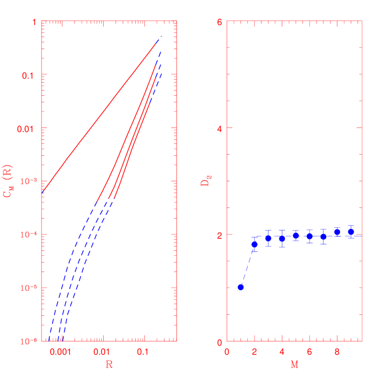
Figure 1: The results of the analysis for $30000$ points from the Rossler system. Left Panel: The $C_{M}(R)$ curves for $M=1,2,5$ and $9$ (from left to right). The solid lines indicate the scaling region which the scheme uses to compute $D_{2}(M)$. Right Panel: The $D_{2}(M)$ values (filled circles). The dashed line is the best fit curve, giving $D_{2}^{sat}=1.97\pm 0.17$.

Table 1:

System	Computed ${D_{2}^{sat}}^{\ast}$	${D_{2}^{sat}}^{\dagger}$
Rossler attractor
$a=b=0.2,c=0.78$	$1.97\pm 0.17$	$1.99\pm 0.08$
Lorenz attractor
$\sigma=10,r=28,b=8/3$	$2.03\pm 0.16$	$2.05\pm 0.1$
Ueda attractor
$k=0.05,A=7.5$	$2.59\pm 0.1$	$2.67\pm 0.13$
Henon map
$a=1.4,b=0.3$	$1.23\pm 0.1$	$1.22\pm 0.04$
Lozi map
$a=1.7,b=0.5$	$1.41\pm 0.1$	$1.38\pm 0.05$
Cat map	$2.00\pm 0.01$	$2.00\pm 0.06$

$\ast$ $D_{2}^{sat}$ values obtained by using the scheme prescribed in this work. For all data sets the number of points used are $30000$

$\dagger$ $D_{2}^{sat}$ taken from [27]

For a randomly generated data set (i.e. white noise), the $D_{2}(M)$ curve goes as $D_{2}(M)=M$ which is also shown in Figure 2. However,for colored random noise characterized by a power-law spectrum, the $D_{2}(M)$ values saturate with $M$. The prescribed scheme should also reproduce effectively $D_{2}^{sat}$ for such non-chaotic systems. This is demonstrated in Figure 3, where the $D_{2}(M)$ curves are plotted for colored noise corresponding to three different values of $\alpha$. In all three cases, the computed values agree with the theoretically expected values.

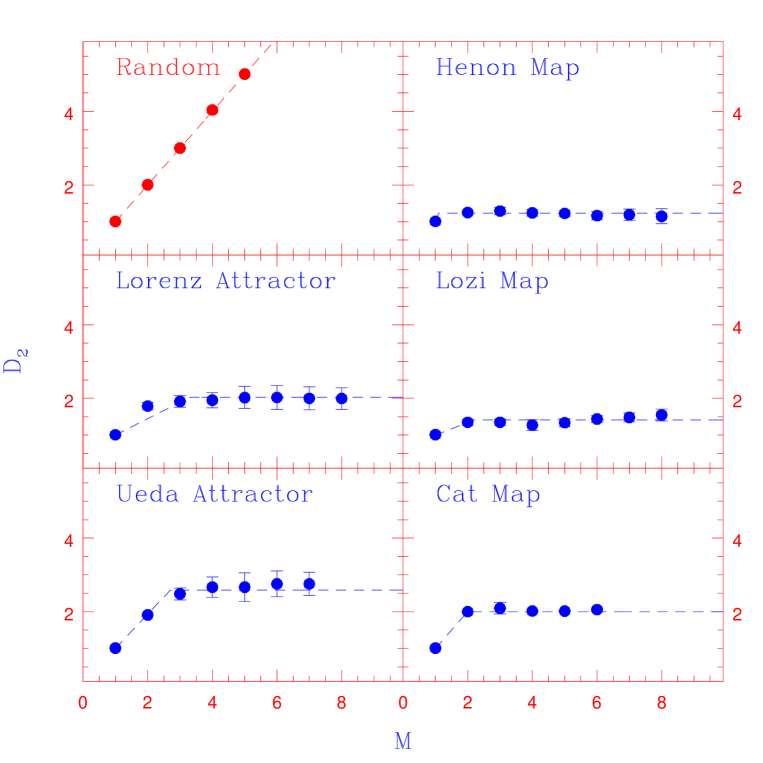
Figure 2: The $D_{2}(M)$ values (filled circles) for random data (white noise) and five standard low dimensional chaotic systems each having $30000$ points. The dashed lines represent the best fit curves giving $D_{2}^{sat}$ values tabulated in Table 1.

The results of the analysis are expected to depend on the number of points in the data stream. As examples, we study the dependence of the computed saturated dimension $D_{2}^{sat}$ on the number of data points available for the Rossler, Ueda and Henon systems. For the flows Rossler and Ueda, the results depend also on the total time $T$ to which the governing differential equations have been evolved. If $T$ is small, then the system would not have traced out its entire attractor region and hence incorrect value of $D_{2}(M)$ would be computed even if the number of points available is large. In Figure 4(a), the variation of $D_{2}^{sat}$ with N are plotted. Here the total time is held constant at $T=300$ and $1500$ for the Rossler and Ueda systems respectively. The data is then sampled at different time intervals $\delta T$, to obtain different values of the number of available points i.e. $N=T/\delta T$. Figure 4(b) shows the dependence of $D_{2}^{sat}$ on the total time $T$, when the number of data points is held constant at $N=10000$. As can be seen in the figure, for the Rossler system, the technique computes reasonable values of $D_{2}^{sat}$ even when $N\sim 1000$, provided the total time $T\geq 300$. However, these values depend on the system and the type of attractor, since for the Ueda system, reasonable values are obtained only when $N\geq 20000$ and the total time $T\geq 800$. This is because of the difference in the inherent Poincare times involved. For maps and colored noise, there is no inherent time-scale in the system and hence the only relevant parameter is the number of data points. The variation of $D_{2}^{sat}$ for the Henon map is also shown in Figure 4(a).

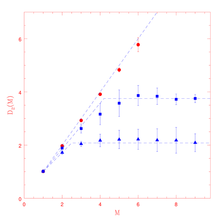
Figure 3: The $D_{2}(M)$ values for colored noise data, each having $30000$ points, corresponding to spectral index $\alpha=1$ (circles), $1.5$ (squares) and $2$ (triangles). The dashed lines are the best fit curves. For $\alpha=1$ the curve is consistent with white noise while for $\alpha=1.5$ and $2.0$, $D_{2}^{sat}=3.75\pm 0.25$ and $2.08\pm 0.16$ respectively. The theoretical value is $D_{2}^{sat}=2/(\alpha-1)$, which gives $\infty$, $4$ and $2$ for $\alpha=1.0$, $1.5$ and $2.0$ respectively

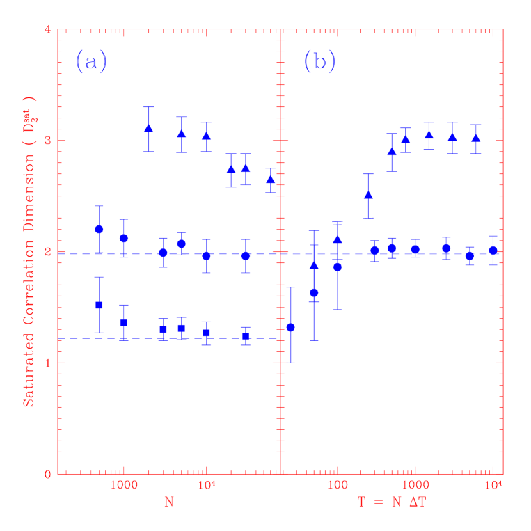
Figure 4: (a) The saturated correlation dimension $D_{2}^{sat}$ versus number of data points $N$ for Ueda (triangles), Rossler (circles) and Henon (squares) system. The total time evolved is $T=N\delta T=300$ and $1500$ for the Rossler and Ueda systems respectively. (b) The saturated correlation dimension $D_{2}^{sat}$ versus the total time $T$ for the Ueda (triangles) and Rossler (circles) system. The total number of points is fixed at $N=10000$. The dashed lines indicate the standard $D_{2}$ values.

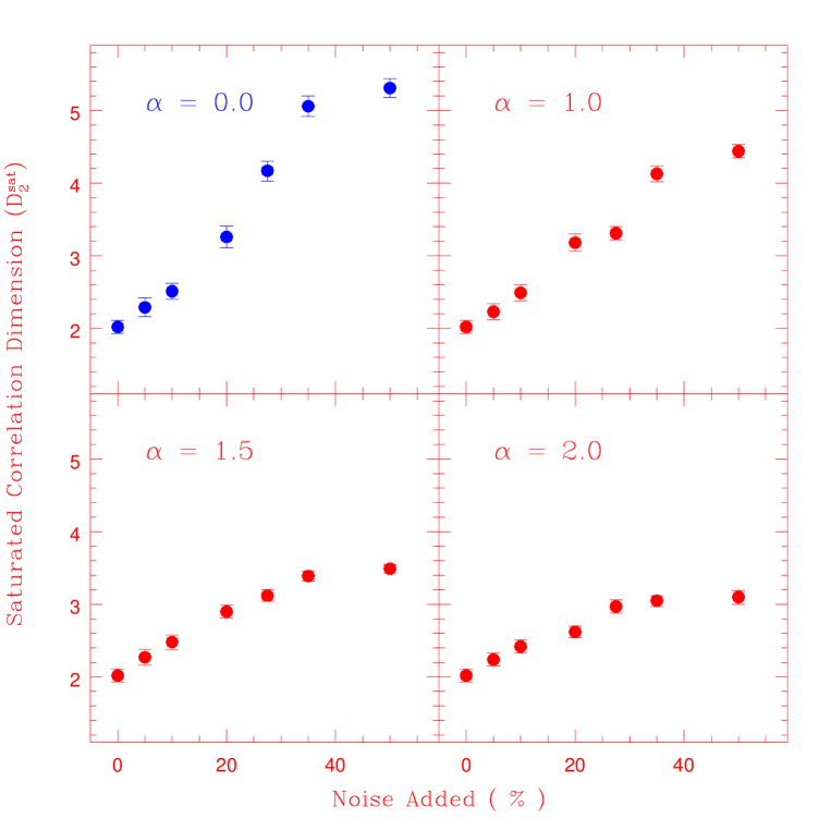
Figure 5: The saturated correlation dimension $D_{2}^{sat}$ for the Rossler system with different percentage of noise added. The four figures correspond to the addition of colored noise with different power spectrum index $\alpha$. For white noise $\alpha=0$ and red noise has $\alpha=2$. The number of points in the data stream is $10000$.

The addition of noise to the data from a chaotic system is expected to increase the value of $D_{2}(M)$. This is illustrated in Figure.5 where $D_{2}^{sat}$ has been plotted for the Rossler system with different percentages of white and colored noise added. Since colored noise has intrinsically low values of $D_{2}(M)$, the increase in $D_{2}^{sat}$ is less for addition of colored noise as compared to white noise. The addition of even 50% red noise ($\alpha=2.0$) increases $D_{2}^{sat}$ only up to $\sim 3$. This emphasizes the need for surrogate data analysis to differentiate between chaotic systems contaminated with noise, from purely stochastic ones.

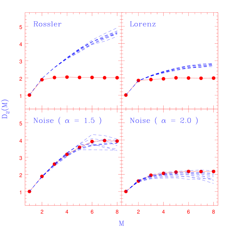
Figure 6: Correlation dimension $D_{2}$ versus $M$, for two chaotic systems ( Rossler and Lorenz) and for colored noise with $\alpha=1.5$ and $2.0$ ( filled circles connected by solid lines). The corresponding $D_{2}(M)$ for ten surrogates are shown by dashed lines. The error bars are omitted for clarity. The normalised mean sigma deviation, $nmsd$ (see text) between the real and surrogate data for the chaotic systems Rossler and Lorenz are $nmsd=36.1$ and $10.2$ respectively, while for the colored noise $nmsd=0.68$ and $2.00$ for $\alpha=1.5$ and $2.0$ respectively.

4 Surrogate Data Analysis

Surrogate data analysis is perhaps the first important analysis that needs to be undertaken on a time series data to detect the presence of non-trivial structures. The basic idea is to formulate a null hypothesis that the data has been created by a stationary linear stochastic process, and then to attempt to reject this hypothesis by comparing results for the data with appropriate realizations of surrogate data. Ideally, surrogate data sets should have the same power spectrum and distribution of values as the real data. The method to generate surrogate data, namely Amplitude Adjusted Fourier Transform (AAFT), was originally proposed by Theiler and co-workers [20]. But recently Schreiber and Schmitz [21, 22] have proposed an iterative scheme, known as IAAFT, which is similar but reported to be more consistent in representing the null hypothesis [35]. In this work, we apply this scheme to generate ten surrogate data sets for each analysis, using the TISEAN package [36,37].

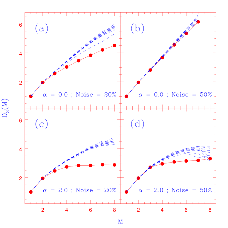
Figure 7: The effect of addition of white ($\alpha=0$) and red noise ($\alpha=2.0$) on surrogate analysis of data from the Rossler system. The $D_{2}(M)$ values for the data are represented by filled circles and connected by solid lines, while for the corresponding ten surrogates, the curves are represented by dashed lines. The upper panel (a) and (b) are for white noise contamination at 20% and 50% reprectively. The lower panel (c) and (d) are for red noise contamination at 20% and 50% reprectively.

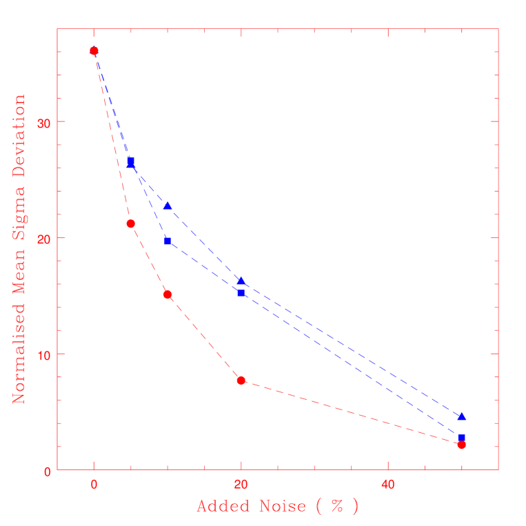
Figure 8: The normalised mean sigma deviation $nmsd$ between data from the Rossler system and ten surrogates versus the percentage of noise added to the data. Circles : white noise ($\alpha=0$); Squares: colored noise ($\alpha=1.5$); Triangles: colored noise ($\alpha=2.0$).

In Figure 6, the $D_{2}(M)$ values for data from two chaotic systems (Rossler and Lorenz) and two kinds of pure colored noise, are shown along with the corresponding surrogates. In all analysis of this section, $10000$ data points are used. As expected the results for the chaotic systems show clear deviation from their surrogates, while for pure colored noise, the results are similar to the surrogates and hence the null hypothesis cannot be rejected. The addition of noise to the chaotic system is found to decrease the difference between the $D_{2}(M)$ of the data and the surrogates. This is shown in Figure 7, where $D_{2}(M)$ for data and surrogates are compared for the Rossler system having different percentages of red colored and white noise added to the time series. Visual inspection of Figure 7 (upper panel), reveals that when white noise is added to the system, $D_{2}(M)$ for both the data and the surrogates increases. There is noticeable difference between the data and surrogates for a contamination level of 20%, but for a larger level of 50%, the data and the surrogates are no longer distinguishable. Red noise contamination is more interesting (Figure 7, lower panel), since for pure red noise (i. e. $\alpha=2.0$) the saturated correlation dimension $D_{2}^{sat}=2$, which is roughly the same as that for the Rossler system. Thus the $D_{2}(M)$ value for surrogates decreases as the percentage of contamination increases, while the $D_{2}(M)$ values for the data increase. Nevertheless, even for a noise added level of 50%, the data and the surrogates are still distinguishable, in contrast to the case when white noise was added to the system. This result has also been verified for other values of $\alpha$.

The above mentioned differences may appear highly qualitative and hence a quantification is attempted by defining a normalised mean sigma deviation, $nmsd$. For this the average of $D_{2}^{surr}(M)$, denoted here as $<D_{2}^{surr}(M)>$, is estimated using a number of realizations of the surrogate data. Then

$$nmsd^{2}=\frac{1}{M_{max}-1}\sum_{M=2}^{M_{max}}\Big{(}\frac{D_{2}(M)-<D_{2}^{surr}(M)>}{\sigma^{surr}_{SD}(M)}\Big{)}^{2}$$ (6)

where $M_{max}$ is the maximum embedding dimension for which the analysis is undertaken and $\sigma^{surr}_{SD}(M)$ is the standard deviation of $D_{2}^{surr}(M)$. The normalised mean sigma deviation, $nmsd=36.1$ and $10.2$ for the Rossler and Lorenz systems respectively, while $nmsd=0.6$ and $2.0$ for the two cases of colored noise (Figure 6). Thus a conservative upper limit of $nmsd=3$ can be imposed, such that when $nmsd$ is greater than $3$, the data can be considered to be distinguishable from its surrogates. The variation of $nmsd$ for different percentages of white and colored noise added to the Rossler system is shown in Figure 8. Note that for the same percentage contamination, $nmsd$ is larger for colored noise than for white noise.

5 Experimental Data Analysis

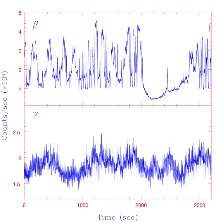
Figure 9: The light curves from two temporal states, $\beta$ and $\gamma$ of the black hole system GRS1915+105, see text for details.

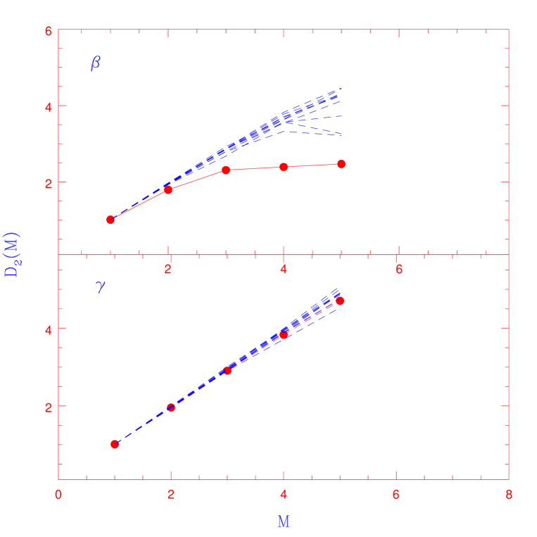
Figure 10: The $D_{2}(M)$ values for the data (filled circles connected by line) and the corresponding values for surrogates (dashed lines) for the states shown in Figure 9

Finally, we consider two data streams each obtained from different real world experiments, one set from an astrophysical X-ray object and the other, EEG data of the human brain. For both these cases, the continuous data stream has $N<5000$ points and is expected to have noise contamination of unknown type and percentage. The X-ray data is taken from GRS 1915+105, which is a highly variable black hole system. Its temporal behavior has been classified into 12 different states and it shows signatures of low dimensional chaotic behavior in some of these states [38]. Here we choose representative data sets from two different spectral classes, namely, the $\beta$ state and the $\gamma$ state, both consisting of 3200 data points. The data has been extracted with a resolution of one second to avoid the effect of Poisson noise. The X-ray light curves are shown in Figure 9, while Figure 10 shows the $D_{2}(M)$ curves for the data and the surrogates in both cases, obtained by applying our scheme. Here the $nmsd$ is found to be 7.02 and 0.89 for $\beta$ and $\gamma$ respectively, indicating that the null hypothesis can be rejected for the $\beta$ state.

There are indications of nonlinear signature in the dynamical properties of the human brain’s electrical activity, particularly during an epileptic seizure. Hence we choose two EEG data sets of the human brain, one during seizure period and the other for healthy state; both consist of 4098 data points. The data has been studied earlier and further details regarding its analysis can be found in Andrzejak et. al [39]. The EEG time series for both cases are shown in Figure 11, and the results of our analysis are shown in Figure 12. The curves are clearly different for the data and the surrogates for the seizure signal with $nmsd=20.1$, while the healthy signal behaves as noise with $nmsd=0.64$, consistent with the earlier analysis in [39].

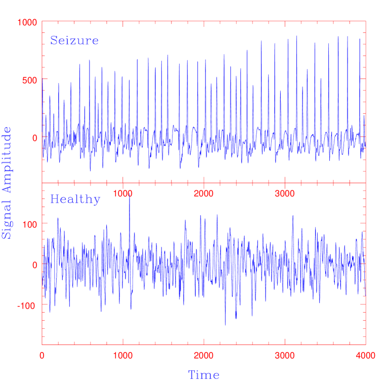
Figure 11: The EEG time series for a seizure period and the healthy state

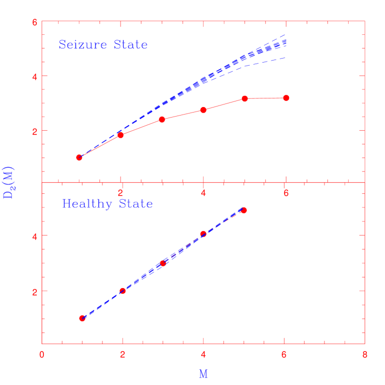
Figure 12: The $D_{2}(M)$ values for the data(filled circles) and the corresponding surrogates for the two EEG time series shown in Figure 11

6 Discussion

In this paper we have implemented a modification of the conventional GP algorithm and calculated the correlation dimension in a non-subjective manner. The method is most suitable for surrogate data analysis where it is imperative that the same conditions are maintained in the algorithm for the data and the surrogates. Moreover, it can be applied to any arbitrary time series with a few thousand data points and provides an error estimate on the value of $D_{2}^{sat}$ obtained.

The scheme is tested for standard low dimensional chaotic systems and for pure colored noise, and it is found that the computed $D_{2}(M)$ are close to the standard values in all cases. As expected, the addition of noise to the data from chaotic systems increases the correlation dimension $D_{2}(M)$. The scheme can differentiate between the results from noise contaminated data and corresponding surrogates, when the percentage of noise addition is low. The level of noise contamination up to which this differentiation can be made depends on the type of noise. The effect of contamination by red noise (which intrinsically has a low saturated correlation dimension) on surrogate data analysis is less compared to the addition of white noise, i. e., for the same percentage of noise addition, data with colored noise is more distinguishable from corresponding surrogates, than data with white noise. This implies that in those practical situations where experimental data have colored (or an unknown type of) noise combined with the real signal, the present scheme can be used effectively. As examples of application, data sets from two scientific experiments are analyzed and the nature of their variability ascertained.

It is also important at this stage to highlight a few possible limitations of this scheme while applying it to specific data sets. The scheme assumes that the actual scaling of $C(R)$ with $R$ is independent of $R$ and hence the limit of $R\rightarrow 0$ is not taken. This is particularly important for those systems where the scaling is significantly different for small and large $R$ values [24]. The method of computing the time delay $\tau$ in this scheme need not be optimal for some specific data sets. Nevertheless, under certain real life conditions, like when the number of data sets are many and/or when a change in the state of a system needs to be evaluated quickly and/or when qualitative differences between time series needs to be estimated, the present scheme is recommended as a useful tool to compute the correlation dimension (and compare with surrogates) without non-algorithmic interventions.

KPH and GA acknowledge the hospitality and facilities in IUCAA. The authors thank the Department of Epileptology, University of Bonn, for making the human brain EEG data available on their website.

References

- [1] P. Grassberger and I. Proccacia, Measuring the Strangeness of Strange Attractors, Physica D9(1983)189.
- [2] P.Grassberger and I.Proccacia, Characterisation of Strange Attractors, Phys.Rev.Lett 50(1983)346.
- [3] T. Schreiber, Inter Disciplinary Applications of Time Series Analysis, Physics Reports 308(1999)1.
- [4] H. D. L. Aberbanel, Analysis of Observed Chaotic Data, (Springer, New York,1996).
- [5] J.C.Sprott, Chaos and Time Series Analysis, (Oxford Univ.Press,New York,2003).
- [6] T. Serre, Z. Kollath and J. R. Buchler, Search for Low Dimensional Nonlinear Behavior in Irregular Variable Stars, Astronomy and Astrophys. 311(1996)833.
- [7] A. Raidl, Estimating the Fractal Dimension,K2 Entropy and Predictability of the Atmosphere, Czeh.J.Phys. 46(1996)293.
- [8] J. B. Ramsey and H. Yuen, Bias and Error Bars in Dimension Calculations and their Evaluation in some Simple Models, Phys.Letters A 134(1988)287.
- [9] J. P. Eckmann, E. Jarvenpaa, M. Jarvenpaa and I. Proccacia, Estimating the Correlation Dimension of the Visible Universe, astro-ph/0301034(2003).
- [10] C. Silva, I. R. Pimentel, A. Andrada, J. P. Fored and E. D. Soares, Correlation Dimension Maps of EEG from Epileptic Absences, Brain Topography 11(1999)201.
- [11] M.Ding,C.Grebogi,E.Ott,T.Sauer and J.A.Yorke, Plateu onset for Correlation Dimension:When does it occur?, Phys.Rev.Lett 70(1993)3872.
- [12] L.A.Smith, Intrinsic limits on Dimension Calculations, Phys.Lett A133(1988)283.
- [13] I.Dvorak and J.Klashka, Modification of the Grassberger-Proccacia Algorithm for estimating Correlation Exponent of Chaotic Systems with high Embedding Dimension, Phys.Lett A145(1990)225.
- [14] M.Casdagli,S.Eubank,J.D.Farmer and J.Gibson, State Space Reconstruction in the presence of Noise, Physica D51(1991)52.
- [15] T.Schreiber, Determination of Noise Level of Chaotic Time Series, Phys.Rev. E48(1993)R13.
- [16] C.Diks, Estimating Invariants of Noisy Attractors, Phys.Rev. E53(1996)4263.
- [17] A. R. Osborne and A. Provenzale, Finite Correlation Dimension for Stochastic Systems with Power-Law Spectra, Physica D 35(1989)357.
- [18] J.Theiler, Some Comments on the Correlation Dimension of noise, Phys.Lett. A155(1991)480.
- [19] S.Redaelli,D.Plewczynski and W.M.Macek, Influence of Colored Noise on Chaotic Systems, Phys.Rev. E 66(2002)035202(R).
- [20] J.Theiler,S.Eubank,A.Longtin,B.Galdrikian and J.D.Farmer, Testing for Nonlinearity in Time Series:The Method of Surrogate Data, Physica D 58(1992)77.
- [21] T.Schreiber and A.Schmitz, Improved Surrogate Data for Nonlinearity Tests, Phys.Rev.Lett. 77(1996)635.
- [22] H.Kantz and T.Schreiber, Nonlinear Time Series Analysis, (Cambridge University Press,Cambridge,1997).
- [23] M.B.Kennel and S.Isabelle, Method to Distinguish Possible Chaos from Colored Noise and to Determine Embedding Parameters, Phys.Rev. A 46(1992)3111.
- [24] K.Judd, An Improved Estimator of Dimension and some Comments on Providing Confidence Intervals, Physica D 56(1992)216.
- [25] M.Small and K.Judd, Detecting Nonlinearity in Experimental Data, Int.J.Bif. Chaos 8(1998)1231.
- [26] K.Judd, Estimating Dimension from Small Samples, Physica D 71(1994)421.
- [27] J. C. Sprott and G. Rowlands, Improved Correlation Dimension Calculation, Int.J.Bif.Chaos 11 (2001) 1865.
- [28] P. Grassberger, Finite Sample Corrections to Entropy and Dimension Estimates, Phys.Letters A 128(1988)369.
- [29] J. B. Ramsey, C. L. Sayers and P. Rothman, The Statistical Properties of Dimension Calculations using Small Data Sets-Economic Applications, Int.Eco.Rev. 31(1990)991.
- [30] D.Yu,M.Small,R.G.Harrison and C.Diks, Efficient Implementation of Gaussian Kernal Algorithm in estimating Invariants and Noise Level from Noisy Time Series Data, Phy.Rev. E61(2000)3750.
- [31] J. Theiler, Efficient Algorithm for Estimating the Correlation Dimension from a Set of Discrete Points, Phys.Rev.A 36(1987)4456.
- [32] G. Nolte, A. Ziehe and K. R. Muller, Noise Robust Estimates of Correlation and K2 Entropy, Phys.Rev.E 64(2001)016112(1-10).
- [33] T. Sander, G. Wubbeler, A. Lueschow, G. Curio and L. Trahms, Nonlinear Time Series Analysis for Human Alpha Rhythm, IEEE Trans.Biomed.Engg. 49(2002)345.
- [34] A.Guerrero and L.A.Smith, Towards Coherent Estimation of Correlation Dimension, Phys.Lett. A318(2003)373.
- [35] D.Kugiumtzis, Test Your Surrogate Data Before You Test for Nonlinearity, Phys.Rev.E 60(1999)2808.
- [36] R.Hegger,H.Kantz and T.Schreiber, Practical Implementation of Nonlinear Time Series Methods:The TISEAN Package, CHAOS 9(1999)413.
- [37] T.Schreiber and A.Schmitz, Surrogate Time Series, Physica D142(2000)346.
- [38] R. Misra, K. P. Harikrishnan, B. Mukhopadhyay, G. Ambika and A. K. Kembhavi, Chaotic Behavior of the Black Hole System GRS1915+105, Astrophys.J. 609(2004)313.
- [39] R.G.Andrzejak,K.Lehnertz,F.Mormann,C.Rieke,P.David and C.E.Elger, Indications of Nonlinear Deterministic and Finite Dimensional Structures in Time Series of Brain Electrical Activity, Phys.Rev.E 64(2001)061907.