Translationally invariant nonlinear Schrödinger lattices

Abstract

Persistence of stationary and traveling single-humped localized solutions in the spatial discretizations of the nonlinear Schrödinger (NLS) equation is addressed. The discrete NLS equation with the most general cubic polynomial function is considered. Constraints on the nonlinear function are found from the condition that the second-order difference equation for stationary solutions can be reduced to the first-order difference map. The discrete NLS equation with such an exceptional nonlinear function is shown to have a conserved momentum but admits no standard Hamiltonian structure. It is proved that the reduction to the first-order difference map gives a sufficient condition for existence of translationally invariant single-humped stationary solutions and a necessary condition for existence of single-humped traveling solutions. Other constraints on the nonlinear function are found from the condition that the differential advance-delay equation for traveling solutions admits a reduction to an integrable normal form given by a third-order differential equation. This reduction also gives a necessary condition for existence of single-humped traveling solutions. The nonlinear function which admits both reductions defines a two-parameter family of discrete NLS equations which generalizes the integrable Ablowitz–Ladik lattice.

1 Introduction

We address spatial discretizations of the nonlinear Schrödinger (NLS) equation in one dimension,

$$iu_{t}+u_{xx}+2|u|^{2}u=0,\qquad x\in\mathbb{R},\quad t\in\mathbb{R}$$ (1.1)

which has a family of traveling wave solutions

$$u=\sqrt{\omega}\;{\rm sech}(\sqrt{\omega}(x-2ct-s))\;e^{ic(x-ct)+i\omega t+i\theta},$$ (1.2)

where $\omega\in\mathbb{R}_{+}$ and $(c,s,\theta)\in\mathbb{R}^{3}$ are free parameters of the solution family. The discrete counterpart of the NLS equation takes the form:

$$i\dot{u}_{n}+\frac{u_{n+1}-2u_{n}+u_{n-1}}{h^{2}}+f(u_{n-1},u_{n},u_{n+1})=0,\qquad n\in\mathbb{Z},\quad t\in\mathbb{R},$$ (1.3)

where $h^{2}>0$ is parameter, and $f:\mathbb{C}^{3}\mapsto\mathbb{C}$ is a non-analytic function with the properties:

• (symmetry) $f(v,u,w)=f(w,u,v)$

• (continuity) $f(u,u,u)=2|u|^{2}u$

• (gauge covariance) $f(e^{i\alpha}v,e^{i\alpha}u,e^{i\alpha}w)=e^{i\alpha}f(v,u,w)$ $\forall\alpha\in\mathbb{R}$

• (reversibility) $\overline{f(v,u,w)}=f(\bar{v},\bar{u},\bar{w})$

We refer to the model (1.3) as the discrete NLS equation or simply the NLS lattice. The discrete NLS equation (1.3) is a symplectic semi-discretization of the continuous NLS equation (1.1), where the second partial derivative is replaced with the second-order central difference on the grid $x=nh$, $n\in\mathbb{Z}$ and the nonlinearity incorporates the effects of on-site and adjacent-site couplings [OWW04]. From another point of view, the discrete model (1.3) is derived in various branches of physics, most recently, in the context of Bose–Einstein condensates in periodic optical lattices [KRB01].

The symmetry property P1 is required to ensure that the semi-discretization is symplectic. The continuity property P2 is needed if the discrete NLS equation (1.3) is to be matched to the continuous NLS equation (1.1) in the limit $h\to 0$. The gauge covariance and reversibility properties P3–P4 originate from applications of the discrete and continuous NLS equations to the modelling of the envelope of modulated nonlinear dispersive waves in a non-dissipative system [KRB01]. We enforce two additional properties on the nonlinear function $f$:

• $f(v,u,w)$ is independent on $h$

• $f(v,u,w)$ is a homogeneous cubic polynomial in $(v,u,w)$

Neither analysis nor applications require properties P5–P6. However, we use them to limit the search of all possible exceptional NLS lattices to a finite-dimensional parameter space. Indeed, we find immediately that all properties P1–P6 are satisfied if and only if the nonlinear function $f(u_{n-1},u_{n},u_{n-1})$ is represented by the ten-parameter family of cubic polynomials,

$$f = \alpha_{1}|u_{n}|^{2}u_{n}+\alpha_{2}|u_{n}|^{2}(u_{n+1}+u_{n-1})+\alpha_{3}u_{n}^{2}(\bar{u}_{n+1}+\bar{u}_{n-1})+\alpha_{4}(|u_{n+1}|^{2}+|u_{n-1}|^{2})u_{n}$$ (1.4)

$$+\alpha_{5}(\bar{u}_{n+1}u_{n-1}+u_{n+1}\bar{u}_{n-1})u_{n}+\alpha_{6}(u_{n+1}^{2}+u_{n-1}^{2})\bar{u}_{n}+\alpha_{7}u_{n+1}u_{n-1}\bar{u}_{n}$$

$$+\alpha_{8}(|u_{n+1}|^{2}u_{n+1}+|u_{n-1}|^{2}u_{n-1})+\alpha_{9}(u_{n+1}^{2}\bar{u}_{n-1}+\bar{u}_{n+1}u_{n-1}^{2})$$

$$+\alpha_{10}(|u_{n+1}|^{2}u_{n-1}+|u_{n-1}|^{2}u_{n+1}),$$

where the real-valued parameters $(\alpha_{1},...,\alpha_{10})$ satisfy the continuity constraint:

$$\alpha_{1}+2\alpha_{2}+2\alpha_{3}+2\alpha_{4}+2\alpha_{5}+2\alpha_{6}+\alpha_{7}+2\alpha_{8}+2\alpha_{9}+2\alpha_{10}=2.$$ (1.5)

This family generalizes the cubic on-site lattice when

$${\rm(dNLS)}\qquad f=2|u_{n}|^{2}u_{n}$$ (1.6)

and the integrable Ablowitz–Ladik (AL) lattice

$${\rm(AL)}\qquad f=|u_{n}|^{2}(u_{n+1}+u_{n-1}).$$ (1.7)

A more general nonlinear function of the form (1.4) was derived in the context of modeling of the Fermi-Pasta-Ulam (FPU) problem (see Eqs. (11)-(12) in [CKKS93]) with

$$\alpha_{1}=\alpha_{2}=\alpha_{4}=\frac{1}{4},\qquad\alpha_{3}=\alpha_{6}=\alpha_{8}=\frac{1}{8},\qquad\alpha_{5}=\alpha_{7}=\alpha_{9}=\alpha_{10}=0.$$ (1.8)

We shall consider persistence of traveling wave solutions (1.2) in the discrete NLS equation (1.3) for sufficiently small $h$ depending on the nonlinear function (1.4). Since both the translational and Gallileo invariances are broken, existence of a stationary solution for some $\omega\in I_{1}\subset\mathbb{R}$,

$$u_{n}(t)=\phi(hn)e^{i\omega t},\qquad\phi:\mathbb{Z}\mapsto\mathbb{C},$$ (1.9)

does not guarantee existence of a traveling solution for some $(\omega,c)\in I_{2}\subset\mathbb{R}^{2}$,

$$u_{n}(t)=\phi(hn-2ct)e^{i\omega t},\qquad\phi:\mathbb{R}\mapsto\mathbb{C},$$ (1.10)

where $\omega$ is frequency and $c$ is velocity of traveling solutions. In both cases (1.9) and (1.10), we are only interested in existence of single-humped localized solutions $\phi(z)$, which correspond to the ${\rm sech}$-solutions (1.2) in the limit $h\to 0$. In what follows, stationary and traveling solutions stand for single-humped localized solutions unless the opposite is explicitly specified. Direct substitutions of (1.9) and (1.10) to the discrete NLS equation (1.3) show that the sequence $\{\phi_{n}\}_{n\in\mathbb{Z}}$ with $\phi_{n}=\phi(hn)$ satisfies the second-order difference equation,

$$\frac{\phi_{n+1}-2\phi_{n}+\phi_{n-1}}{h^{2}}-\omega\phi_{n}+f(\phi_{n-1},\phi_{n},\phi_{n+1})=0,\quad n\in\mathbb{Z},$$ (1.11)

while the function $\phi(z)$ with $z=hn-2ct$ satisfies the differential advance-delay equation,

$$2ic\phi^{\prime}(z)=\frac{\phi(z+h)-2\phi(z)+\phi(z-h)}{h^{2}}-\omega\phi(z)+f(\phi(z-h),\phi(z),\phi(z+h)),\quad z\in\mathbb{R}.$$ (1.12)

Existence of stationary solutions of the second-order difference equation (1.11) can be established for a large class of nonlinearities (1.4) by using the variational method [P05]. Two single-humped solutions exist in a general case: one solution is symmetric about a selected lattice node (say $n=0$) and the other solution is symmetric about a midpoint between two adjacent nodes.

There are two obstacles for the stationary solution (1.9) to persist as the traveling solution (1.10). First, the solution of the stationary problem (1.11) corresponds generally to a piecewise continuous solution $\phi(z)$ of the traveling problem (1.12) on $z\in\mathbb{R}$ [AEHV05]. Jump discontinuities of $\phi(z)$ may occur in between two adjacent nodes, e.g. between $z_{n}=hn$ and $z_{n+1}=(n+1)h$. Second, even if there exists a continuous solution $\phi(z)$ of the traveling problem (1.12) with $c=0$, this solution may not persist as a continuously differentiable solution $\phi(z)$ of the problem (1.12) with $c\neq 0$. The stationary solution of the second-order difference equation (1.11) is said to be translationally invariant if the function $\phi_{n}=\phi(nh)$ on $n\in\mathbb{Z}$ can be extended to a one-parameter family of continuous solutions $\phi(z-s)$ on $z\in\mathbb{R}$ of the advance-delay equation (1.12) with $c=0$, where $s\in\mathbb{R}$ is an arbitrary translation parameter.

The persistence problem for traveling waves in discrete lattices was recently considered in a number of publications. Kevrekidis [K03] suggested a method to define an exceptional nonlinear function $f(u_{n-1},u_{n},u_{n+1})$ from the condition that the discrete NLS equation (1.3) preserves the momentum invariant,

$$M=i\sum_{n\in\mathbb{Z}}\left(\bar{u}_{n+1}u_{n}-u_{n+1}\bar{u}_{n}\right).$$ (1.13)

No characterization of the nonlinear functions (1.4) that preserve the momentum conservation (1.13) was made in [K03] except for the integrable AL lattice (1.7). In addition, it was not shown in [K03] that the preservation of momentum (1.13) guarantees the existence of a continuous function $\phi(z)$ in the solution (1.10) with $c=0$.

Oster, Johansson, and Eriksson [OJE03] addressed the most general Hamiltonian discrete NLS equation in the form,

$$i\dot{u}_{n}=\frac{\partial H}{\partial\bar{u}_{n}},\qquad H=\sum_{n\in\mathbb{Z}}\left(\frac{|u_{n+1}-u_{n}|^{2}}{h^{2}}-F(u_{n},u_{n+1})\right),$$ (1.14)

where $F:\mathbb{C}^{2}\mapsto\mathbb{R}$ is a symmetric potential function of quartic polynomials which satisfies the gauge invariance property: $F(e^{i\alpha}u,e^{i\alpha}w)=F(u,w)$ $\forall\alpha\in\mathbb{R}$. The dNLS lattice (1.6) and the FPU lattice (1.8) are particular examples of the Hamiltonian discrete NLS equation (1.14). It was found in [OJE03] that there exists a configuration in parameters of quartic polynomials $F(u_{n},u_{n+1})$ which provides a reduced Peierls–Nabarro potential and enhanced mobility of localized modes. No analysis of the localized modes with enhanced mobility was developed in [OJE03].

Ablowitz and Musslimani [AM03] outlines problems in the numerical approximations for traveling wave solutions (1.10) with $c\neq 0$ in the context of earlier contradictory publications (see also review in [PR05]). An asymptotic method was developed in [AM03] to show that if the solution exists for $c=0$ it can be continued to non-zero values of $c$ as perturbation series expansions in powers of $c$.

Pelinovsky and Rothos [PR05] computed the normal form for bifurcations of traveling solutions (1.10) near the special value of the parameter $c=1/h$. The normal form is represented by the third-order ODE related to the third-order derivative NLS equation [PR05]. Existence of embedded solitons in the third-order derivative NLS equation was considered in the past (see [YA03, PY05] and reference therein) and the previous results suggested that the dNLS lattice (1.6) did not support bifurcation of single-humped traveling solutions in a sharp contrast to the case of the AL lattice (1.7). (Double-humped traveling solutions in the normal form reduction were predicted for the dNLS lattice (1.6) in [PR05] and numerical approximations of the double-humped traveling solutions in the differential advance-delay equation (1.12) were obtained in [C06].)

We shall review the results and conjectures of the previous works [AM03, K03, OJE03, PR05] in the context of the cubic nonlinear function (1.4). Our results are based on the recent works [BOP05] and [DKY05], where similar ideas are developed for monotonic kinks of the discrete $\phi^{4}$ theory. See also [OPB05, IP06] for other relevant results on monotonic kinks in discrete Klein–Gordon lattices.

In Section 2, the class of exceptional nonlinear functions in the general family of cubic polynomials (1.4) is identified from the condition that the second-order difference equation (1.11) admits a reduction to the first-order difference equation. It is shown that the discrete NLS equation (1.3) with an exceptional nonlinearity preserves the momentum conservation (1.13) but admits no Hamiltonian in the form (1.14).

In Section 3, it is proved that the first-order difference equation admits a one-parameter family of stationary solutions (1.9) for any $\omega>0$ and sufficiently small $h$, and these stationary solutions are translationally invariant. Unlike the case of monotonic kinks in [BOP05], the proof of existence of a translationally invariant single-humped localized solution is based on a construction of two sequences which depend continuously on the initial value. One sequence is monotonically decreasing to zero and the other sequence is monotonically increasing until the turning point and it decreases monotonically beyond the turning point. The main outcome of this analysis is a clear evidence that the reduction to the first-order difference equation gives a sufficient condition for existence of translationally invariant stationary solutions and a necessary condition for existence of traveling solutions near $c=0$ for $\omega>0$.

Section 4 tests the exceptional nonlinear functions by the reduction of the differential advance-delay equation (1.12) to the normal form near the special values of parameters $\omega=(\pi-2)/h^{2}$ and $c=1/h$. Reductions of the normal form to integrable Hirota [H73] and Sasa-Satsuma [SS91] equations and existence of single-humped solutions in the integrable normal form give a necessary condition for existence of traveling solutions in the differential advance-delay equation (1.12) near the special values of parameters $(\omega,c)$.

Section 5 presents the explicit form of the two-parameter exceptional nonlinear function (1.4) that passes through both tests and may contain families of traveling solutions. This function generalizes the AL lattice (1.7) which is known to admit exact traveling solutions between the two limits $c=0$ and $c=1/h$. Numerical test of persistence of traveling solutions in the differential advance-delay equation (1.12) is outlined as an open problem.

2 Reductions to the first-order difference equation

We shall consider the stationary solution (1.9) of the discrete NLS equation (1.3), which satisfies the second-order difference equation (1.11). We obtain the constraints on the function $f(\phi_{n-1},\phi_{n},\phi_{n+1})$ in the family of cubic polynomials (1.4) from the condition that the second-order difference equation (1.11) admits a conserved quantity

$$E=\frac{1}{h^{2}}|\phi_{n+1}-\phi_{n}|^{2}-\frac{1}{2}\omega\left(\phi_{n}\bar{\phi}_{n+1}+\bar{\phi}_{n}\phi_{n+1}\right)+g(\phi_{n},\phi_{n+1}),$$ (2.1)

where $g:\mathbb{C}^{2}\mapsto\mathbb{R}$ is a non-analytic function and $E\in\mathbb{R}$ is constant in $n\in\mathbb{Z}$. Due to properties P1–P6 for the function $f(\phi_{n-1},\phi_{n},\phi_{n+1})$, the nonlinear function $g(\phi_{n},\phi_{n+1})$ satisfies the properties:

• (symmetry) $g(u,w)=g(w,u)$

• (continuity) $g(u,u)=|u|^{4}$ and $\frac{\partial g}{\partial\bar{u}}(u,u)=\frac{\partial g}{\partial\bar{w}}(u,u)=|u|^{2}u$

• (gauge variance) $g(e^{i\alpha}u,e^{i\alpha}w)=g(u,w)$ $\forall\alpha\in\mathbb{R}$

• (reversibility) $\overline{g(u,w)}=g(\bar{u},\bar{w})$

• $g(u,w)$ is independent on $h$

• $g(u,w)$ is a homogeneous quartic polynomial in $(u,w)$

The most general polynomial $g(\phi_{n},\phi_{n+1})$ that satisfies properties S1–S6 takes the form:

$$g = \gamma_{1}(|\phi_{n}|^{2}+|\phi_{n+1}|^{2})(\bar{\phi}_{n+1}\phi_{n}+\phi_{n+1}\bar{\phi}_{n})+\gamma_{2}|\phi_{n}|^{2}|\phi_{n+1}|^{2}$$ (2.2)

$$+\gamma_{3}(\phi_{n}^{2}\bar{\phi}_{n+1}^{2}+\bar{\phi}_{n}^{2}\phi_{n+1}^{2})+\gamma_{4}(|\phi_{n}|^{4}+|\phi_{n+1}|^{4}),$$

where the real-valued parameters $(\gamma_{1},\gamma_{2},\gamma_{3},\gamma_{4})$ satisfy the continuity constraint:

$$4\gamma_{1}+\gamma_{2}+2\gamma_{3}+2\gamma_{4}=1.$$ (2.3)

In the limit $h\to 0$, the second-order difference equation (1.11) reduces to the second-order ODE:

$$\phi^{\prime\prime}-\omega\phi+2|\phi|^{2}\phi=0,$$ (2.4)

while the first-order difference equation (2.1) transforms to the first integral of (2.4)

$$E=|\phi^{\prime}|^{2}-\omega|\phi|^{2}+|\phi|^{4}.$$ (2.5)

The first-order ODE (2.5) with $E=0$ admits a unique localized solution $\phi(z)=\sqrt{\omega}\;{\rm sech}(\sqrt{\omega}(z-s))$ with $s\in\mathbb{R}$ and $\omega>0$, which agrees with the exact solution (1.2) for $z=x$ and $c=0$. Therefore, the first-order difference equation (2.1) is a symplectic discretization of the first-order ODE (2.5). This precise methodology was used in [DKY05] to construct translationally invariant monotonic kinks in the discrete $\phi^{4}$ equation. (A more general approach is reported in [BOP05].) We first specify on the correspondence between the difference equations (1.11) and (2.1) and then prove three elementary results on existence of the reduction (2.1) with the nonlinear function (2.2) and its relation to conservation of $M$ in (1.13) and $H$ in (1.14).

Lemma 2.1

Let the function $g(\phi_{n},\phi_{n+1})$ with properties S1–S6 be related to the function $f(\phi_{n-1},\phi_{n},\phi_{n+1})$ with properties P1–P6 by

$$g(\phi_{n},\phi_{n+1})-g(\phi_{n-1},\phi_{n})=\frac{1}{2}\left[(\bar{\phi}_{n+1}-\bar{\phi}_{n-1})f(\phi_{n-1},\phi_{n},\phi_{n+1})+(\phi_{n+1}-\phi_{n-1})\overline{f(\phi_{n-1},\phi_{n},\phi_{n+1})}\right].$$

If the sequence $\{\phi_{n}\}_{n\in\mathbb{Z}}$ is any solution of the second-order difference equation (1.11), it satisfies the first-order difference equation (2.1). If the sequence $\{\phi_{n}\}_{n\in\mathbb{Z}}$ is a non-constant real-valued solution of the first-order difference equation (2.1), it also satisfies the second-order difference equation (1.11).

• Proof. By subtracting the first-order difference equation (2.1) with $n\equiv n$ from that with $n\equiv n-1$, we have

  $$\frac{1}{2}(\bar{\phi}_{n+1}-\bar{\phi}_{n-1})\left(\frac{\phi_{n+1}-2\phi_{n}+\phi_{n-1}}{h^{2}}-\omega\phi_{n}\right)$$

  $$+\frac{1}{2}(\phi_{n+1}-\phi_{n-1})\left(\frac{\bar{\phi}_{n+1}-2\bar{\phi}_{n}+\bar{\phi}_{n-1}}{h^{2}}-\omega\bar{\phi}_{n}\right)+g(\phi_{n},\phi_{n+1})-g(\phi_{n-1},\phi_{n})=0.$$ (2.6)

  The first statement follows immediately from the relation between $f(\phi_{n-1},\phi_{n},\phi_{n+1})$ and $g(\phi_{n},\phi_{n+1})$. Let us now assume that the first-order equation (2.1) is satisfied and functions $f(\phi_{n-1},\phi_{n},\phi_{n+1})$ and $g(\phi_{n},\phi_{n+1})$ are related as above. Then, the non-constant sequence $\{\phi_{n}\}_{n\in\mathbb{Z}}$ satisfies the second-order equation,

  $$\frac{\phi_{n+1}-2\phi_{n}+\phi_{n-1}}{h^{2}}-\omega\phi_{n}+f(\phi_{n-1},\phi_{n},\phi_{n+1})=i(\phi_{n+1}-\phi_{n-1})h(\phi_{n-1},\phi_{n},\phi_{n+1}),\quad n\in\mathbb{Z},$$

  where $h:\mathbb{C}^{3}\mapsto\mathbb{R}$ is arbitrary function. If the non-constant sequence is also real-valued, then $h\equiv 0$.  

Remark 2.2

The one-to-one correspondence between the second-order and first-order difference equations (1.11) and (2.1) exists only for non-constant real-valued solutions. Complex-valued solutions of the first-order equation (2.1) can give solutions of the second-order equation with an additional function $h(\phi_{n-1},\phi_{n},\phi_{n+1})$. This property can be used for a full time-space discretization of the NLS equation (1.1), when the derivative term $\phi^{\prime}(z)$ in the differential advance-delay equation (1.12) is replaced by the difference term $(\phi_{n+1}-\phi_{n-1})/(2h)$ such that the function $h(\phi_{n-1},\phi_{n},\phi_{n+1})=c/h$ is constant. We will not consider full time-space discretizations of the NLS equation (1.1) in this paper.

Lemma 2.3

The reduction of the second-order difference equation (1.11) to the first-order difference equation (2.1) exists provided that the nonlinear function (1.4) satisfies the constraints:

$$\alpha_{4}=\alpha_{1}-\alpha_{6},\qquad\alpha_{5}=\alpha_{6},\qquad\alpha_{7}=\alpha_{1}-2\alpha_{6},\qquad\alpha_{10}=\alpha_{8}-\alpha_{9},$$ (2.7)

such that $(\alpha_{1},\alpha_{2},\alpha_{3},\alpha_{6},\alpha_{8},\alpha_{9})\in\mathbb{R}^{6}$ are free parameters.

• Proof. By using symbolic computations with Wolfram’s Mathematica we find from (1.4), (2.2) and (2.6) that $\alpha_{1}=2\gamma_{1}$, $\alpha_{2}=\gamma_{2}$, $\alpha_{3}=2\gamma_{3}$, and $\alpha_{8}=\gamma_{4}$ under the constraints (2.7).  

Corollary 2.4

When $\phi_{n}\in\mathbb{R}$, the first-order difference equation (2.1) is characterized by the symmetric quartic polynomial function

$$g=\beta_{1}\phi_{n}^{2}\phi_{n+1}^{2}+\beta_{2}(\phi_{n}^{2}+\phi_{n+1}^{2})\phi_{n}\phi_{n+1}+\beta_{3}(\phi_{n}^{4}+\phi_{n+1}^{4}),$$ (2.8)

where $\beta_{1}=\gamma_{2}+2\gamma_{3}=\alpha_{2}+\alpha_{3}$, $\beta_{2}=2\gamma_{1}=\alpha_{1}$, and $\beta_{3}=\gamma_{4}=\alpha_{8}$ under the continuity constraint

$$\beta_{1}+2\beta_{2}+2\beta_{3}=1.$$ (2.9)

Remark 2.5

Corollary 2.9 recovers the result of [BOP05], where real-valued nonlinear functions of the difference equation (1.11) are considered in the context of kink solutions of the discrete $\phi^{4}$ model.

Lemma 2.6

The discrete NLS equation (1.3) conserves the momentum invariant (1.13) provided that the constraints (2.7) are met.

• Proof. Computing time-derivative of (1.13) and using the stroboscopical summation in $n$, we convert the result to the following irreducible remainder:

  $$\dot{M} = (\alpha_{1}-\alpha_{4}-\alpha_{6})\sum_{n\in\mathbb{Z}}(|u_{n+1}|^{2}-|u_{n}|^{2})(u_{n+1}\bar{u}_{n}+\bar{u}_{n+1}u_{n}))$$

  $$+ (\alpha_{4}-\alpha_{5}-\alpha_{7})\sum_{n\in\mathbb{Z}}(|u_{n+1}|^{2}(u_{n}\bar{u}_{n-1}+\bar{u}_{n}u_{n-1})-|u_{n-1}|^{2}(u_{n}\bar{u}_{n+1}+\bar{u}_{n}u_{n+1}))$$

  $$+ (\alpha_{5}-\alpha_{6})\sum_{n\in\mathbb{Z}}(u_{n+1}u_{n}\bar{u}_{n-1}^{2}+\bar{u}_{n+1}\bar{u}_{n}u_{n-1}^{2}-u_{n+1}^{2}\bar{u}_{n}\bar{u}_{n-1}-\bar{u}_{n+1}^{2}u_{n}u_{n-1})$$

  $$+ (\alpha_{8}-\alpha_{9}-\alpha_{10})\sum_{n\in\mathbb{Z}}(|u_{n+1}|^{2}-|u_{n-1}|^{2})(u_{n+1}\bar{u}_{n-1}+\bar{u}_{n+1}u_{n-1}).$$

  The constraints (2.7) give the most general solution of the system of homogeneous linear equations, which follows from the momentum conservation $\dot{M}=0$.  

Corollary 2.7

There exists a one-to-one correspondence between the set of nonlinear functions (1.4) that conserves the momentum (1.13) and the set of nonlinear functions that supports the reduction to the first-order difference equation (2.1).

Remark 2.8

Corollary 2.7 proves the conjecture of [K03] for the case of a discrete NLS equation (1.3) with the cubic polynomial function (1.4). A similar result for a discrete Klein–Gordon equation was obtained in the most general case in [K03, Appendix] by explicit computations.

Lemma 2.9

The discrete NLS equation (1.3) has the Hamiltonian structure (1.14) provided that

$$\alpha_{2}=2\alpha_{3}=2\alpha_{8},\qquad\alpha_{5}=\alpha_{7}=\alpha_{9}=\alpha_{10}=0,$$ (2.10)

such that $(\alpha_{1},\alpha_{2},\alpha_{4},\alpha_{6})\in\mathbb{R}^{4}$ are free parameters.

• Proof. The most general symmetric real-valued gauge-invariant function $F(u_{n},u_{n+1})$ of the quartic polynomials in the Hamiltonian (1.14) takes the form:

  $$F = \delta_{1}(|u_{n}|^{2}+|u_{n+1}|^{2})(u_{n}\bar{u}_{n+1}+\bar{u}_{n}u_{n+1})+\delta_{2}|u_{n}|^{2}|u_{n+1}|^{2}$$

  $$+\delta_{3}(u_{n}^{2}\bar{u}_{n+1}^{2}+\bar{u}_{n}^{2}u_{n+1}^{2})+\delta_{4}(|u_{n}|^{4}+|u_{n+1}|^{4}).$$

  Due to the symplectic structure (1.14), the potential function $F(u_{n},u_{n+1})$ produces the nonlinear function $f(u_{n-1},u_{n},u_{n+1})$ in the form,

  $$f = \delta_{1}\left[|u_{n+1}|^{2}u_{n+1}+|u_{n-1}|^{2}u_{n-1}+2|u_{n}|^{2}(u_{n+1}+u_{n-1})+u_{n}^{2}(\bar{u}_{n+1}+\bar{u}_{n-1})\right]$$

  $$+\delta_{2}(|u_{n+1}|^{2}+|u_{n-1}|^{2})u_{n}+2\delta_{3}(u_{n+1}^{2}+u_{n-1}^{2})\bar{u}_{n}+4\delta_{4}|u_{n}|^{2}u_{n}.$$

  Therefore, $\alpha_{2}=2\delta_{1}$, $\alpha_{4}=\delta_{2}$, $\alpha_{6}=2\delta_{3}$ and $\alpha_{1}=4\delta_{4}$ under the constraints (2.10).  

Corollary 2.10

None of the discrete NLS equations with the Hamiltonian structure (1.14) is momentum-preserving, including the dNLS lattice (1.6) and the FPU lattice (1.8).

Remark 2.11

Corollary 2.10 agrees with the conclusion of [DKY05] obtained for the discrete $\phi^{4}$ model.

Remark 2.12

The three-parameter discrete NLS equation with the Hamiltonian structure (1.14) was derived in [OJE03] for modeling of arrays of optical waveguides. The model of [OJE03] corresponds to the reduction of the symmetric potential function $F(u_{n},u_{n+1})$ with $\delta_{2}=4\delta_{3}$. Although it is claimed in [OJE03] from results of numerical simulations that traveling solutions may have enhanced mobility in this model, no momentum-preservation is supported and the second-order difference equation (1.11) provides no reduction to the first-order difference equation (2.1).

3 Existence of translationally invariant stationary solutions

We shall consider existence of continuous solutions of the advance-delay equation (1.12) with $c=0$ from existence of the translationally invariant solutions of the second-order difference equation (1.11). We show that there exist translationally invariant stationary solutions if the second-order difference equation (1.11) is reduced to the first-order difference equation (2.1). Thus, the existence of the reduction to the first-order difference equation (2.1) gives the sufficient condition for existence of translationally invariant stationary solutions. For simplicity, the analysis is developed for real-valued solutions of the first-order difference equation (2.1). By Lemma 2.1, such non-constant solutions correspond to real-valued solutions of the second-order difference equation (1.11). The initial-value problem for the first-order difference equation (2.1) with $E=0$ in the space of real-valued localized solutions takes the implicit form,

$$\left\{\begin{array}[]{l}(\phi_{n+1}-\phi_{n})^{2}=h^{2}\omega\phi_{n}\phi_{n+1}-h^{2}g(\phi_{n},\phi_{n+1}),\qquad n\in\mathbb{Z},\\ \phi_{0}=\varphi,\end{array}\right.$$ (3.1)

where $\varphi\in\mathbb{R}$ is the initial data, iterations in both positive and negative directions of $n\in\mathbb{Z}$ are considered, and $g:\mathbb{R}^{2}\mapsto\mathbb{R}$ is given by (2.8). Let $x=\phi_{n}$ and $y=\phi_{n+1}$ and rewrite $g(\phi_{n},\phi_{n+1})$ as

$$g(x,y)=\beta_{1}x^{2}y^{2}+\beta_{2}xy(x^{2}+y^{2})+\beta_{3}(x^{4}+y^{4}).$$

Due to the continuity constraint (2.9), we have $g(x,x)=x^{4}$ and $\partial_{x}g(x,x)=\partial_{y}g(x,x)=2x^{3}$. We first establish the sufficient condition that the second-order difference equation (1.11) has only real-valued solutions and then develop analysis of the initial-value problem (3.1) in $n\in\mathbb{Z}$. Our main result is Proposition 3.13 which guarantees existence of a particular single-humped localized sequence $\{\phi_{n}\}_{n\in\mathbb{Z}}$ to the initial-value problem (3.1) with $\omega>0$ and sufficiently small $h$. The sequence corresponds to the translationally invariant solution of the second-order equation (1.11) which converges as $h\to 0$ to the solution $\phi_{s}(z)=\sqrt{\omega}\;{\rm sech}(\sqrt{\omega}z)$ at the points $z=hn$ with $n\in\mathbb{Z}$.

Lemma 3.1

The second-order difference equation (1.11) with sufficiently small $h$ admits a conserved quantity

$$J=\bar{\phi}_{n}\phi_{n+1}-\phi_{n}\bar{\phi}_{n+1}$$ (3.2)

for bounded sequences $\{\phi_{n}\}_{n\in\mathbb{Z}}$ if

$$\alpha_{7}=2\alpha_{6},\qquad\alpha_{10}=\alpha_{8}+\alpha_{9}.$$ (3.3)

• Proof. The nonlinear function (1.4) satisfies the relation

  $$\bar{\phi}_{n}f(\phi_{n-1},\phi_{n},\phi_{n+1})-\phi_{n}\overline{f(\phi_{n-1},\phi_{n},\phi_{n+1})}=\left(\bar{\phi}_{n}\phi_{n+1}-\phi_{n}\bar{\phi}_{n+1}+\bar{\phi}_{n}\phi_{n-1}-\phi_{n}\bar{\phi}_{n-1}\right)Q_{n}+R_{n}$$

  where

  $$Q_{n}=(\alpha_{2}-\alpha_{3})|\phi_{n}|^{2}+\alpha_{8}(|\phi_{n-1}|^{2}+|\phi_{n+1}|^{2})+\alpha_{9}(\bar{\phi}_{n-1}\phi_{n+1}+\phi_{n-1}\bar{\phi}_{n+1})$$

  $$+\alpha_{6}(\bar{\phi}_{n}\phi_{n+1}+\phi_{n}\bar{\phi}_{n+1}+\bar{\phi}_{n}\phi_{n-1}+\phi_{n}\bar{\phi}_{n-1})$$

  and

  $$R_{n}=(\alpha_{7}-2\alpha_{6})(\bar{\phi}_{n}^{2}\phi_{n-1}\phi_{n+1}-\phi_{n}^{2}\bar{\phi}_{n-1}\bar{\phi}_{n+1})$$

  $$+(\alpha_{10}-\alpha_{8}-\alpha_{9})\left[(\bar{\phi}_{n}\phi_{n-1}-\phi_{n}\bar{\phi}_{n-1})|\phi_{n+1}|^{2}+(\bar{\phi}_{n}\phi_{n+1}-\phi_{n}\bar{\phi}_{n+1})|\phi_{n-1}|^{2}\right].$$

  If $\alpha_{7}=2\alpha_{6}$ and $\alpha_{10}=\alpha_{8}+\alpha_{9}$, then $R_{n}\equiv 0$. If the sequence $\{\phi_{n}\}_{n\in\mathbb{Z}}$ is bounded, then $1+h^{2}Q_{n}>0$ and $J$ is constant for all $n\in\mathbb{Z}$ provided that $h$ is sufficiently small.  

Corollary 3.2

Under the constraints (3.3), real-valued solutions of the second-order difference equation (1.11) with $J=0$ are the only localized bounded solutions $\{\phi_{n}\}_{n\in\mathbb{Z}}$ with $\phi_{0}\in\mathbb{R}$.

Remark 3.3

While it is not clear if localized complex-valued solutions of the second-order difference equation (1.11) may exist when $\alpha_{7}\neq 2\alpha_{6}$ and $\alpha_{10}\neq\alpha_{8}+\alpha_{9}$, we observe that the reduction to the first-order difference equation (2.1) has six free parameters (see Lemma 2.3) but the nonlinear function in the form (2.2) has only four parameters. Therefore, two parameters can be used to satisfy the constraints (3.3). Combining the constraints (2.7) and (3.3), we obtain the most general parameterization of the nonlinear function (1.4) that admits the conserved quantities (2.1) and (3.2):

$$\alpha_{1}=4\alpha_{6},\quad\alpha_{4}=3\alpha_{6},\quad\alpha_{5}=\alpha_{6},\quad\alpha_{7}=2\alpha_{6},\quad\alpha_{9}=0,\quad\alpha_{10}=\alpha_{8},$$ (3.4)

where $(\alpha_{2},\alpha_{3},\alpha_{6},\alpha_{8})\in\mathbb{R}^{4}$ are free parameters. By Lemma 2.1 and Corollary 3.2, all localized non-constant solutions of the second-order difference equation (1.11) under the constraints (3.4) are real-valued and the sequence $\{\phi_{n}\}_{n\in\mathbb{Z}}$ is equivalently found from the initial-value problem (3.1).

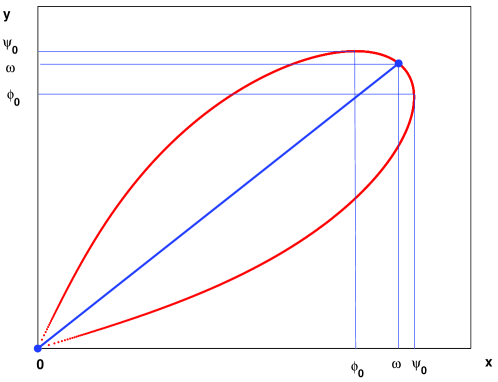
Figure 1: Solutions of the quartic equation (3.5) with $\beta_{1}=\beta_{2}=0$ and $\beta_{3}=0.5$.

Lemma 3.4

Let $Q(x,y)=\omega xy-g(x,y)$ and $\omega>0$ is parameter. There exists $h_{0}>0$ and $L>\sqrt{\omega}$ such that the algebraic (quartic) equation

$$(y-x)^{2}=h^{2}Q(x,y)$$ (3.5)

defines a convex, simply-connected, closed curve inside the domain $0\leq x\leq L$ and $0\leq y\leq L$ for $0<h<h_{0}$. The curve is symmetric about the diagonal $y=x$ and has two intersections with the diagonal at $y=x=0$ and $y=x=\sqrt{\omega}$.

• Proof. The statement of lemma is illustrated on Figure 1. Symmetry of the curve about the diagonal $y=x$ follows from the fact that $g(x,y)=g(y,x)$. Intersections with the diagonal $y=x$ follows from the continuity constraint that gives $Q(x,x)=x^{2}(\omega-x^{2})$. To prove convexity, we consider the behavior of the curve for sufficiently small $h$ in two domains: in the interval $0\leq x\leq x_{0}$ and in a small neighborhood of the point $y=x=\sqrt{\omega}$ with the radius $r_{0}h^{2}$, where $x_{0}=\sqrt{\omega}-r_{0}h^{2}$ and $r_{0}>\frac{\sqrt{\omega^{3}}}{8}$ is $h$-independent. Let $y=x+z$ and consider two branches of the algebraic equation (3.5) in the implicit form

  $$F_{\pm}(x,z,h)=z\mp h\sqrt{Q(x,x+z)}=0.$$ (3.6)

  such that for $x\geq 0$

  $$F_{\pm}(x,0,h)=\mp hx\sqrt{\omega-x^{2}},\qquad\partial_{z}F_{\pm}(x,0,h)=1\mp\frac{h(\omega-2x^{2})}{2\sqrt{\omega-x^{2}}}.$$

  It is clear that $F_{\pm}(x,0,0)=0$ and $\partial_{z}F_{\pm}(x,0,0)=1$, while $F_{\pm}(x,0,h)$ is continuously differentiable in $x$ and $h$ and $\partial_{z}F_{\pm}(x,0,h)$ is uniformly bounded in $x$ and $h$ on any compact subset of $x\in[0,x_{0}]$, where $x_{0}=\sqrt{\omega}-r_{0}h^{2}$ and $r_{0}>\frac{\sqrt{\omega^{3}}}{8}$ is $h$-independent. By the Implicit Function Theorem, there exists $h_{0}>0$, such that the implicit equations (3.6) define unique roots $z=\pm hS_{\pm}(x,h)$ in the domain $0\leq x\leq x_{0}$ and $0<h<h_{0}$, where $hS_{\pm}(x,h)$ are positive, continuously differentiable functions in $x$ and $h$. Therefore, the algebraic equation (3.5) defines two branches of the curve located above and below the diagonal $y=x$. When $h_{0}$ is sufficiently small, the two branches are strictly increasing in the interval $0\leq x\leq x_{0}$. In the limit $h_{0}\to 0$, the two branches converge to the diagonal $y=x$ on $0\leq x\leq\sqrt{\omega}$. Derivatives of the algebraic equation (3.5) in $x$ are defined for any branch of the curve by

  $$y^{\prime}\left[2(y-x)-h^{2}(\omega x-\partial_{y}g(x,y))\right] = 2(y-x)+h^{2}(\omega y-\partial_{x}g(x,y)),$$ (3.7)

  $$y^{\prime\prime}\left[2(y-x)-h^{2}(\omega x-\partial_{y}g(x,y))\right] = -2(y^{\prime}-1)^{2}+h^{2}(2\omega y^{\prime}-\tilde{g}),$$ (3.8)

  where $\tilde{g}=\partial^{2}_{xx}g(x,y)-2y^{\prime}\partial^{2}_{xy}g(x,y)-(y^{\prime})^{2}\partial^{2}_{yy}g(x,y)$. It follows from the first derivative (3.7) that $y^{\prime}=-1$ at the point $y=x=\sqrt{\omega}$ for any $h>0$, such that there exists a small neighborhood of the point $y=x=\sqrt{\omega}$ where the upper branch of the curve is strictly decreasing. Let $B_{h}^{+}$ be the upper semi-disk centered at $y=x=\sqrt{\omega}$ with a radius $r_{0}h^{2}$, where $r_{0}>\frac{\sqrt{\omega^{3}}}{8}$ is $h$-independent. Then, there exists a $h$-independent constant $C>0$ such that

  $$2(y-x)-h^{2}(\omega x-\partial_{y}g(x,y))\geq Ch^{2},\qquad(x,y)\in B_{h}^{+}.$$

  It follows from the second derivative (3.8) for sufficiently small $h$ that $y^{\prime\prime}\leq-C_{1}/h^{2}$ in $(x,y)\in B_{h}^{+}$ with $C_{1}>0$. Therefore, the curve is convex in $B_{h}^{+}$. By using the rescaled variables in $B_{h}^{+}$:

  $$x=\sqrt{\omega}-Xh^{2},\qquad y=\sqrt{\omega}+Yh^{2},$$

  we find that the curvature of the curve in new variables is bounded by $Y^{\prime\prime}(X)\leq-C_{1}$ and therefore, the first derivative $Y^{\prime}(X)$ and so $y^{\prime}(x)$ may only change by a finite number in $(x,y)\in B_{h}$. Therefore, there exists $0<C_{2}<\infty$ such that $y^{\prime}(x)=C_{2}$ at a point $x$, where $x\leq x_{0}=\sqrt{\omega}-r_{0}h^{2}$. By the first part of the proof, the upper branch of the curve is monotonically increasing for $0\leq x\leq x_{0}$. By the second part of the proof, it has a single maximum for $x_{0}\leq x\leq\sqrt{\omega}$. Thus, the curve defined by the quartic equation (3.5) is convex for $y\geq x\geq 0$ (and for $0\leq y\leq x$ by symmetry).  

Corollary 3.5

Let $\psi_{0}$ be a maximal value of $y$ and $\varphi_{0}$ be the corresponding value of $x$ on the upper branch of the curve defined by the quartic equation (3.5). Then, $\varphi_{0}<\sqrt{\omega}<\psi_{0}$ and

$$\varphi_{0}=\sqrt{\omega}-\frac{3}{8}\sqrt{\omega^{3}}h^{2}+{\rm O}(h^{4}),\qquad\psi_{0}=\sqrt{\omega}+\frac{1}{8}\sqrt{\omega^{3}}h^{2}+{\rm O}(h^{4}).$$ (3.9)

Lemma 3.6

The initial-value problem (3.1) with $\omega>0$ and $0<h<h_{0}$ admits a unique monotonically decreasing sequence $\{\phi_{n}\}_{n=0}^{\infty}$ for any $0<\varphi<\sqrt{\omega}$ that converges to zero from above as $n\to\infty$. The sequence $\{\phi_{n}\}_{n=0}^{\infty}$ is continuous with respect to $h$ and $\varphi$.

• Proof. By Lemma 3.4 (see Figure 1), there exists a unique lower branch of the curve in (3.5) below the diagonal $y=x$ for $0<x<\sqrt{\omega}$ and the monotonically decreasing sequence $\{\phi_{n}\}_{n=0}^{\infty}$ with $0<\varphi<\sqrt{\omega}$ satisfies the initial-value problem:

  $$\left\{\begin{array}[]{l}\phi_{n+1}=\phi_{n}-hS_{-}(\phi_{n},h),\qquad n\in\mathbb{N}\\ \phi_{0}=\varphi\end{array}\right.$$ (3.10)

  where $hS_{-}(\phi,h)>0$ is continuously differentiable with respect to $\phi$ and $h$. We shall prove that the monotonically decreasing sequence $\{\phi_{n}\}_{n=0}^{\infty}$ converges to zero from above. Since $Q(x,y)$ is a quartic polynomial, there exists a constant $C>0$ that depends on $\omega$ and is independent of $h$, such that

  $$(\phi_{n+1}-\phi_{n})^{2}\leq Ch^{2}\phi_{n}^{2}$$ (3.11)

  for all $\phi_{n+1}<\phi_{n}$. If $h$ is sufficiently small, such that $Ch^{2}<1$, then $0<\phi_{n+1}<\phi_{n}$, and the sequence $\{\phi_{n}\}_{n=0}^{\infty}$ is bounded from below by $\phi=0$. By the Weierstrass Theorem, the monotonically decreasing and bounded from below sequence $\{\phi_{n}\}_{n=0}^{\infty}$ converges as $n\to\infty$ to the fixed point $\phi=0$. Continuity of the sequence $\{\phi_{n}\}_{n=0}^{\infty}$ in $h$ and $\varphi$ follows from smoothness of $hS_{-}(\phi,h)$ in $h$ and $\varphi$.  

Lemma 3.7

There exists $N\geq 1$, such that the initial-value problem (3.1) with $\omega>0$ and $0<h<h_{0}$ admits a unique monotonically increasing sequence $\{\phi_{n}\}_{n=-\infty}^{N}$ for any $0<\varphi<\sqrt{\omega}$ that converges to zero from above as $n\to-\infty$. The sequence $\{\phi_{n}\}_{n=-\infty}^{N}$ is continuous with respect to $h$ and $\varphi$.

• Proof. By Lemma 3.4 (see Figure 1), there exists a unique upper branch of the curve in (3.5) above the diagonal $y=x$ for $0<x<\sqrt{\omega}$ and the monotonically increasing sequence $\{\phi_{n}\}_{n=-\infty}^{0}$ with $0<\varphi<\sqrt{\omega}$ satisfies the initial-value problem:

  $$\left\{\begin{array}[]{l}\phi_{n+1}=\phi_{n}+hS_{+}(\phi_{n},h),\qquad(-n)\in\mathbb{N}\\ \phi_{0}=\varphi\end{array}\right.$$ (3.12)

  where $hS_{+}(\phi,h)>0$ is continuously differentiable with respect to $\phi$ and $h$. Existence of $N\geq 1$ follows from the same equation (3.12) for $0\leq n\leq N-1$. The proof that the monotonically increasing sequence $\{\phi_{n}\}_{n=-\infty}^{N}$ converges to zero from above as $n\to-\infty$ is similar to the proof of Lemma 3.6. Continuity of the sequence $\{\phi_{n}\}_{n=-\infty}^{N}$ in $h$ and $\varphi$ follows from smoothness of $hS_{+}(\phi,h)$ in $h$ and $\varphi$.  

Lemma 3.8

The initial-value problem (3.1) with $\omega>0$ and $0<h<h_{0}$ admits a unique 2-periodic orbit $\{\phi_{n}\}_{n\in\mathbb{Z}}$ with $\phi_{n+1}\neq\phi_{n}$ and $\phi_{n+2}=\phi_{n}$ for any $\varphi_{0}<\varphi<\psi_{0}$.

• Proof. By Lemma 3.4 (see Figure 1), the curve in (3.5) is symmetric about $y=x$ and has two branches in $x$ below $y=x$ for $\sqrt{\omega}<x<\psi_{0}$. Therefore, any initial data on the branch between $(\varphi_{0},\psi_{0})$ and $(\psi_{0},\varphi_{0})$ leads to a unique 2-periodic orbit.  

Corollary 3.9

The initial-value problem (3.1) with $\omega>0$ and $0<h<h_{0}$ admits the following particular sequences:

• For any given $0<\varphi\leq\psi_{0}$, there exists a symmetric single-humped sequence $\{\phi_{n}\}_{n\in\mathbb{Z}}$ with maximum at $n=0$, such that $\phi_{n}=\phi_{-n}$ (see Figure 2(a)). The single-humped sequence is unique for $\varphi=\psi_{0}$ (see Figure 2(b)). Let $S_{\rm on}$ denote the countable infinite set of values of $\{\phi_{n}\}_{n\in\mathbb{Z}}$ for the single-humped solution with $\varphi=\psi_{0}$.

• For any given $\sqrt{\omega}<\varphi<\psi_{0}$, there exists a symmetric double-humped sequence $\{\phi_{n}\}_{n\in\mathbb{Z}}$ with local minimum at $n=1$ and maxima at $n=0$ and $n=2$, such that $\phi_{n}=\phi_{-n+2}$ and $\varphi_{0}<\phi_{1}<\sqrt{\omega}$ (see Figure 3(a)). The double-humped sequence becomes a unique $2$-site top single-humped sequence for $\varphi=\sqrt{\omega}$ (see Figure 3(b)). Let $S_{\rm off}$ denote the countable infinite set of values of $\{\phi_{n}\}_{n\in\mathbb{Z}}$ for the $2$-site top single-humped solution with $\varphi=\sqrt{\omega}$.

• For any $\varphi\in(0,\psi_{0})\backslash\{S_{\rm on},S_{\rm off}\}$, there exists a unique non-symmetric single-humped sequence $\{\phi_{n}\}_{n\in\mathbb{Z}}$ with $\phi_{k}\neq\phi_{m}$ for all $k\neq m$.

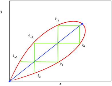
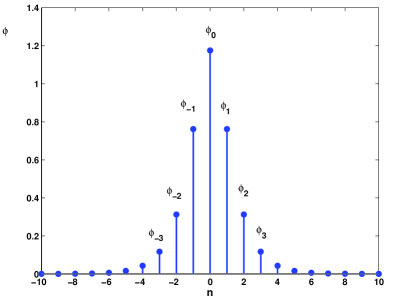
Figure 2: Left: a construction of the symmetric single-humped sequence from the solution of the quartic equation (3.5). Right: an example of the symmetric single-humped solution of the difference equation (3.1) for $\varphi=\psi_{0}$.

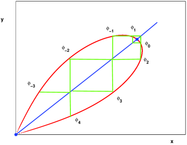
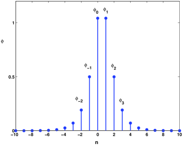
Figure 3: Left: a construction of the symmetric double-humped sequence from the solution of the quartic equation (3.5). Right: an example of the 2-site top single-humped solution of the difference equation (3.1) for $\varphi=\sqrt{\omega}$.

Proposition 3.10

The second-order difference equation (1.11) admits a translationally invariant single-humped sequence $\{\phi_{n}\}_{n\in\mathbb{Z}}$ for any $0<\phi_{0}\leq\psi_{0}$ with $\phi_{n}=\phi(nh-s)$, where $n\in\mathbb{Z}$, $s\in\mathbb{R}$, and $\phi(z)$ is a continuous function. In the limit $h\to 0$, the function $\phi(z)$ converges pointwise to the function $\phi_{s}(z)=\sqrt{\omega}\;{\rm sech}(\sqrt{\omega}z)$, i.e. there exists $C>0$ and $s\in\mathbb{R}$ such that

$$\max_{n\in\mathbb{Z}}|\phi_{n}-\phi_{s}(nh-s)|\leq Ch^{2}.$$ (3.13)

• Proof. By the geometric construction of Corollary 3.9, there exists a single-humped sequence $\{\phi_{n}\}_{n\in\mathbb{Z}}$ for any $0<\phi_{0}\leq\psi_{0}$, which consists of the unique symmetric sequence for $\phi_{0}\in S_{\rm on}$, the unique $2$-site top sequence for $\phi_{0}\in S_{\rm off}$ and the unique non-symmetric sequence for $\phi_{0}\in(0,\psi_{0})\backslash\{S_{\rm on},S_{\rm off}\}$. By Lemmas 3.6 and 3.7, the single-humped sequence is continuous in $h$ and $\phi_{0}$ such that it is translationally invariant. By Lemma 2.1, the real-valued non-constant sequence satisfies identically the second-order equation (1.11). It remains to show the pointwise convergence of the sequence $\{\phi_{n}\}_{n\in\mathbb{Z}}$ to the sequence $\{\phi_{s}(nh-s)\}_{n\in\mathbb{Z}}$ as $h\to 0$, where $\phi_{s}(z)=\sqrt{\omega}\;{\rm sech}(\sqrt{\omega}z)$. By the translational invariance of the sequence, we can place the maximum at $n=0$, such that $\phi_{0}=\psi_{0}$, which is equivalent to the choice $s=0$. Then, the bound (3.13) with $s=0$ coincides with the bound for the convergence of the symmetric single-humped solution with $\{\phi_{n}\}_{n\in\mathbb{Z}}=S_{\rm on}$ of the second-order difference equation (1.11) to the solution $\phi_{s}(hn)=\sqrt{\omega}\;{\rm sech}(\sqrt{\omega}hn)$ of the second-order ODE (2.4). The standard proof of the error bound (3.13) is performed with a formal power series in $h^{2}$ which involves hyperbolic functions for exponentially decaying solutions (see Appendix B in [BGKM91]). The formal series is different from the rigorous convergent asymptotic solution of the difference map (1.11) along the stable and unstable manifolds by the exponentially small in $h$ terms (see [T00] for application of this technique to the second-order difference equation with a quadratic nonlinearity). We note that a similar result (but with a different technique based on analysis of Fourier transforms) was proved in [FP99] for the discrete Fermi–Pasta–Ulam problem.  

Example 3.11

Let us consider the explicit example of the AL lattice (1.7), when $\beta_{1}=1$ and $\beta_{2}=\beta_{3}=0$. In this case, the second-order difference equation (1.11) admits the exact solution for translationally invariant single-humped solutions:

$$\phi_{n}=\psi_{0}\;{\rm sech}(\kappa hn-s),$$ (3.14)

where $(s,\kappa)\in\mathbb{R}^{2}$ are arbitrary and $(\psi_{0},\omega)$ are defined by

$$\psi_{0}=\frac{\sinh(\kappa h)}{h},\qquad\omega=\frac{4}{h^{2}}\sinh^{2}\left(\frac{\kappa h}{2}\right).$$ (3.15)

The set $S_{\rm on}$ for the symmetric single-humped solution is defined by values of $\{\phi_{n}\}_{n\in\mathbb{Z}}$ for $s=0$ (see Figure 2(b)) and the set $S_{\rm off}$ for the 2-site top single-humped solution is defined for $s=\frac{\kappa h}{2}$. We find that

$$\psi_{0}=\sqrt{\omega}\cosh\left(\frac{\kappa h}{2}\right)=\sqrt{\omega+\frac{\omega^{2}h^{2}}{4}},$$ (3.16)

in agreement with the asymptotic formula (3.9). The algebraic equation (3.5) can be reduced to the explicit roots for the one-step maps $hS_{\pm}(\phi,h)$ in the form:

$$S_{\pm}(\phi,h)=\frac{\phi(\sqrt{4(\omega-\phi^{2})+h^{2}\omega^{2}}\pm h(\omega-2\phi^{2}))}{2(1+h^{2}\phi^{2})},$$

which satisfy all properties derived in Lemma 3.4. In particular $S_{+}(\phi,h)>0$ for $0<\phi<\sqrt{\omega}$ and $S_{-}(\phi,h)>0$ has one root for $0<\phi<\sqrt{\omega}$ and two roots for $\sqrt{\omega}<\phi<\psi_{0}$, where $\psi_{0}$ is given by (3.16). In the limit $h\to 0$, the expression (3.14) with (3.15) converges to the solution (1.2) with $\omega=\kappa^{2}$ and $c=0$.

Remark 3.12

For real-valued non-constant solutions, the second-order difference equation (1.11) can be reduced to another first-order difference equation:

$$\frac{1}{h}(\phi_{n+1}-\phi_{n})=\tilde{g}(\phi_{n},\phi_{n+1}),$$ (3.17)

where $\tilde{g}(\phi_{n},\phi_{n+1})$ is a symmetric quadratic polynomial. The form (3.17) was used in [BOP05] in a search of another family of exceptional discretizations which admits translationally invariant monotonic kinks in the discrete $\phi^{4}$ equation. By the Implicit Function Theorem, the first-order difference equation (2.1) has only one branch of solutions on the plane $(\phi_{n},\phi_{n+1})$. As a result, one can not construct two (decreasing and increasing) sequences $\{\phi_{n}\}_{n=0}^{\infty}$ in the first-order difference equation (3.17) for translationally invariant single-humped solutions. Therefore, other exceptional discretizations of [BOP05] are irrelevant for localized solutions of the discrete NLS equation (1.3).

4 Existence of traveling solutions near $\omega=(\pi-2)/h^{2}$ and $c=1/h$

We shall consider existence of continuously differentiable solutions of the differential advance-delay equation (1.12) with $c\neq 0$. A convenient parametrization of the solution is represented by the transformation of variables

$$\phi(z)=\frac{1}{h}\Phi(Z)e^{i\beta Z},\qquad Z=\frac{z}{h},$$ (4.1)

and parameters

$$\omega=\frac{2}{h}\beta c+\frac{2}{h^{2}}\left(\cos\beta\;\cosh\kappa-1\right),\qquad c=\frac{1}{h\kappa}\sin\beta\;\sinh\kappa,$$ (4.2)

such that the parameter $h$ is scaled out the new equation for $\Phi(Z)$:

$$2i\sin\beta\frac{\sinh\kappa}{\kappa}\Phi^{\prime}(Z)+2\cos\beta\cosh\kappa\Phi(Z)$$

$$=\Phi(Z+1)e^{i\beta}+\Phi(Z-1)e^{-i\beta}+f\left(\Phi(Z-1)e^{-i\beta},\Phi(Z),\Phi(Z+1)e^{i\beta}\right),\quad Z\in\mathbb{R}.$$

If the single-humped localized solutions to the differential advance-delay equation exist, then the function $\Phi(Z)$ decays in $Z$ with the real-valued rate $\kappa$, i.e. $\Phi(Z)\sim e^{-\kappa|Z|}$. (Near the bifurcation line $\kappa=0$, the function $\Phi(Z)$ may also contain decaying exponential terms with oscillatory tails due to presence of complex eigenvalues but these terms decay faster than the tail $\Phi(Z)\sim e^{-\kappa|Z|}$.) The boundary on possible existence of traveling solutions corresponds to the line $\kappa=0$, such that the traveling solutions may only exist in the exterior domain to the curve

$$\omega=\frac{2}{h}\beta c-\frac{4}{h^{2}}\sin^{2}\frac{\beta}{2},\qquad c=\frac{1}{h}\sin\beta,\qquad\beta\in[0,2\pi].$$ (4.3)

The boundary on existence of traveling solutions is shown on Figure 4 for $c\geq 0$. We apply the technique of the normal form reduction from [PR05] when parameters $(\omega,c)$ are close to the special values $\omega=(\pi-2)/h^{2}$ and $c=1/h$, which correspond to $\beta=\pi/2$. By using a modified transformation of variables and parameters

$$\phi(z)=\frac{\epsilon}{h}\Phi(\zeta)\;e^{\frac{i\pi z}{2h}},\qquad\zeta=\frac{\epsilon z}{h},\qquad c=\frac{1+\epsilon^{2}V}{h},\qquad\omega=\frac{\pi-2+\epsilon^{2}\pi V+\epsilon^{3}\Omega}{h^{2}},$$

we rewrite the differential advance-delay equation (1.12) in the equivalent form,

$$i\left(\Phi(\zeta+\epsilon)-\Phi(\zeta-\epsilon)-2\epsilon\Phi^{\prime}(\zeta)\right)=\epsilon^{3}\left(2iV\Phi^{\prime}(\zeta)+\Omega\Phi(\zeta)\right)-\epsilon^{2}f(-i\Phi(\zeta-\epsilon),\Phi(\zeta),i\Phi(\zeta+\epsilon)),$$

where $(\Omega,V)\in\mathbb{R}^{2}$ are rescaled parameters $(\omega,c)\in I_{2}\subset\mathbb{R}^{2}$ and properties P3 and P6 of the function $f(v,u,w)$ are used. The small parameter $\epsilon>0$ defines deviation of parameters $(\omega,c)$ from the values $\omega=(\pi-2)/h^{2}$ and $c=1/h$ as well as the amplitude and localization of the solution $\phi(z)$. By using the formal Taylor series expansions of the shift operators $\Phi(\zeta\pm\epsilon)$ in powers of $\epsilon$, the differential advance-delay equation for $\Phi(\zeta)$ is converted to a third-order ODE which is related to the third-order derivative NLS equation [PR05]. The formal reduction can be proved with the rigorous technique of the center manifold and normal forms (see analysis in [IP06] for kinks in the discrete $\phi^{4}$ equation).

The formal reduction of the linear and nonlinear parts of the differential advance-delay equation for $\Phi(\zeta)$ leads to the expansions,

$$\Phi(\zeta+\epsilon)-\Phi(\zeta-\epsilon)-2\epsilon\Phi^{\prime}(\zeta)=\frac{\epsilon^{3}}{3}\Phi^{\prime\prime\prime}(\zeta)+{\rm O}(\epsilon^{5}),$$

and

$$f(-i\Phi(\zeta-\epsilon),\Phi(\zeta),i\Phi(\zeta+\epsilon))=\left(\alpha_{1}+2\alpha_{4}-2\alpha_{5}-2\alpha_{6}+\alpha_{7}\right)|\Phi|^{2}\Phi$$

$$+2i\epsilon\left(\alpha_{2}+2\alpha_{8}-2\alpha_{9}\right)|\Phi|^{2}\Phi^{\prime}(\zeta)-2i\epsilon\left(\alpha_{3}-\alpha_{8}-\alpha_{9}+\alpha_{10}\right)\Phi^{2}\bar{\Phi}^{\prime}(\zeta)+{\rm O}(\epsilon^{2}).$$

By rescaling the amplitude of $\Phi(\zeta)$ one can bring the term $|\Phi|^{2}\Phi$ to the order of $\epsilon^{3}$. However, the third-order ODE

$$\frac{i}{3}\Phi^{\prime\prime\prime}-2iV\Phi^{\prime}-\Omega\Phi=|\Phi|^{2}\Phi,$$

has no single-humped localized solutions for any $(\Omega,V)\in\mathbb{R}^{2}$ (see references in [YA03, PR05]). Therefore, the necessary condition for existence of single-humped traveling solutions is the constraint on parameters of the cubic polynomial function (1.4):

$$\alpha_{1}+2\alpha_{4}-2\alpha_{5}-2\alpha_{6}+\alpha_{7}=0.$$ (4.4)

When other constraints (2.7) and (3.3) are taken into account, the new constraint produces $\alpha_{6}=0$ in the representation (3.4). Under the constraints (2.7), (3.3), and (4.4) and the normalization (1.5), no rescaling of the amplitude of $\Phi(\zeta)$ is needed and the truncated normal form for traveling solutions becomes

$$\frac{i}{3}\Phi^{\prime\prime\prime}-2iV\Phi^{\prime}-\Omega\Phi+2i|\Phi|^{2}\Phi^{\prime}+i\gamma\Phi(|\Phi|^{2})^{\prime}=0,$$ (4.5)

where $\gamma=-2\alpha_{3}=2(\alpha_{2}+2\alpha_{8}-1)$ is a real parameter. Existence of single-humped localized solutions in the third-order ODE (4.5) is related to existence of embedded solitons in the third-order derivative NLS equation (see recent survey in [PY05]). We shall represent the basic facts about existence of single-humped localized solutions of the third-order ODE (4.5). By using the transformation of variables and parameters

$$\Phi=\lambda\Psi(Z)e^{-ikz},\qquad Z=\lambda\zeta,\qquad\Omega=\frac{2}{3}k\left(\lambda^{2}+k^{2}\right),\qquad V=\frac{1}{6}\left(\lambda^{2}-3k^{2}\right),$$

we rewrite the ODE (4.5) in the form,

$$\frac{i\lambda}{3}\left(\Psi^{\prime\prime\prime}-\Psi^{\prime}+6|\Psi|^{2}\Psi^{\prime}+3\gamma\Psi(|\Psi|^{2})^{\prime}\right)+k\left(\Psi^{\prime\prime}-\Psi+2|\Psi|^{2}\Psi\right)=0,$$ (4.6)

where the real-valued parameters $(\lambda,k)$ are arbitrary. The value $\lambda=0$ defines the bifurcation cutoff in the family of localized solutions of the ODE (4.6), which is equivalent to the curve $V=V_{\rm thr}(\Omega)$ in the parameter plane $(\Omega,V)$, where

$$V_{\rm thr}(\Omega)=-\frac{(3\Omega)^{2/3}}{2^{5/3}}.$$ (4.7)

Localized solutions may only exist above the threshold $V>V_{\rm thr}(\Omega)$ for any $\Omega\in\mathbb{R}$. The asymptotic approximation of the threshold (4.7) is shown on Figure 4 by dotted curve. The threshold (4.7) is an asymptotic approximation of the exact curve (4.3).

• When $\gamma=0$, the third-order ODE (4.6) is related to the integrable Hirota equation [H73], which admits the exact single-humped localized solution $\Psi={\rm sech}(Z)$. The single-humped solution exists everywhere on the two-parameter plane $(\Omega,V)$ above the threshold (4.7).

• When $\gamma=1$, the third-order ODE (4.6) is related to the integrable Sasa-Satsuma equation [SS91], which also admits the exact localized solutions everywhere on the two-parameter plane $(\Omega,V)$ above the threshold (4.7). (The exact solution and its properties are given in Sections 4-5 of [SS91].) The localized solution has a single-humped profile for $V_{\rm thr}(\Omega)<V<V_{\rm humps}(\Omega)$ and a double-humped profile for $V>V_{\rm humps}(\Omega)$ and $\Omega\neq 0$, where

  $$V_{\rm humps}(\Omega)=-\frac{(3\Omega)^{2/3}}{32^{4/3}}.$$ (4.8)

  The threshold (4.8) in the ODE (4.6) corresponds to the condition $\lambda^{2}=k^{2}$. It is shown on Figure 4 by dashed-dotted curve. When $\Omega\to 0$ and $V>0$, the distance between two humps diverge and the ODE (4.6) has again the single-humped solution for $\Omega=0$ and $V>0$ with $\Psi=\frac{1}{\sqrt{2}}{\rm sech}(Z)$. This solution corresponds to $k=0$ in the ODE (4.6).

• When $\gamma\in\mathbb{R}$, the third-order ODE (4.5) has the exact single-humped localized solution for $\Omega=0$ and $V>0$ with $\Psi=\frac{1}{\sqrt{1+\gamma}}{\rm sech}(Z)$. The exact solution matches the member of the family of exact solutions in the two integrable cases $\gamma=0$ and $\gamma=1$. It is shown in [PY05] by numerical analysis of the kernel of the linearization operator (see Sections 3-4 in [PY05]) that the family of single-humped localized solutions for $\gamma\in\mathbb{R}\backslash\{0,1\}$ is isolated from other families of localized solutions, i.e. the one-parameter family with $\Omega=0$ and $V>0$ can not be continued in the two-parameter plane $(\Omega,V)$ as a single-humped localized solution.

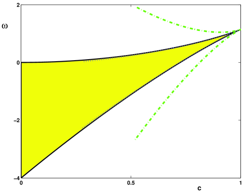
Figure 4: The boundary (4.3) of the domain of existence for traveling solutions of the differential advance-delay equation (1.12) and asymptotic approximations for the threshold on existence (4.7) (dotted curve) and the threshold on two-humped solutions (4.8) (dashed-dotted curve).

Results of the third-order ODE (4.5) give only necessary condition on existence of traveling single-humped solution in the differential advance-delay equation (1.12) near the special values $\omega=(\pi-2)/h^{2}$ and $c=1/h$, i.e. if the smooth solution $\phi(z)$ to the differential advance-delay equation (1.12) exists, then it matches the analytical solutions of the third-order ODE (4.5). Persistence proof of true localized solutions is a delicate problem of rigorous analysis, which is left open even for traveling kinks of the discrete $\phi^{4}$ equation [IP06]. (For comparison, persistence of solutions with exponentially small non-localized oscillatory tails was rigorously proved near the normal form equation in [IP06].)

When the discrete NLS equation (1.3) is the integrable AL lattice (1.7), the exact traveling solutions exist in the form $\Phi(Z)=\sinh\kappa\;{\rm sech}(\kappa Z)$ for any $\kappa>0$ and $\beta\in[0,2\pi]$. These solutions match the exact solutions for the Hirota equation for $V>V_{\rm thr}(\Omega)$ and $\Omega\in\mathbb{R}$ in the form $\Psi(\zeta)={\rm sech}(\zeta)$ with the correspondence $\kappa=\epsilon\lambda$. Additionally, when the discrete NLS equation (1.3) has the nonlinear function

$$f=(1-\alpha)|u_{n}|^{2}(u_{n+1}+u_{n-1})+\alpha u_{n}^{2}(\bar{u}_{n+1}+\bar{u}_{n-1}),\qquad\alpha\neq 0,$$

the exact traveling solution exists for $\kappa>0$ and $\beta=\frac{\pi}{2}$ in the form

$$\Phi(Z)=\frac{1}{\sqrt{1-2\alpha}}\sinh\kappa\;{\rm sech}(\kappa Z).$$

This solution matches the exact solution of the third-order ODE (4.5) for $\Omega=0$ and $V>0$ in the form $\Psi(\zeta)=\frac{1}{\sqrt{1+\gamma}}{\rm sech}(Z)$ (where $\gamma=-2\alpha_{3}$ and $\alpha=\alpha_{3}$). We do not know if there are any other examples of the discrete NLS equation (1.3) with the nonlinear function (1.4) which admit families of single-humped traveling solutions which match the analytical solutions of the third-order ODE (4.5). See [BGH04] for symbolic tests of explicit $\tanh$ and ${\rm sech}$ solutions of differential advance-delay equations.

5 Conclusion

We have considered stationary and traveling solutions of the discrete NLS equation (1.3) with the ten-parameter cubic nonlinearity (1.4) under the normalization constraint (1.5). We have proved in Lemma 2.3 that four constraints (2.7) are sufficient for reduction of the second-order difference equation (1.11) to the first-order difference equation (2.1). The main result (Proposition 3.13) says that this reduction gives a sufficient condition for existence of translationally invariant stationary solutions that converge to the stationary solutions (1.2) with $c=0$ in the continuum limit $h\to 0$.

Furthermore, we have proved in Lemma 3.3 that two additional constraints (3.3) are sufficient for uniqueness of real-valued stationary localized solutions in the first-order difference equation (2.1). We have finally found in Section 4 that one more constraint gives the necessary condition for existence of traveling solutions in the differential advance-delay equation (1.12) near the special values $\omega=(\pi-2)/h^{2}$ and $c=1/h$. Combining all constraints (2.7), (3.3), and (4.4) and the normalization constraint (1.5), we have a two-parameter family of the discrete NLS equation with the nonlinear function

$$f=(1-\alpha-2\beta)|u_{n}|^{2}(u_{n+1}+u_{n-1})+\alpha u_{n}^{2}(\bar{u}_{n+1}+\bar{u}_{n-1})+\beta(|u_{n+1}|^{2}+|u_{n-1}|^{2})(u_{n+1}+u_{n-1}),$$ (5.1)

where $(\alpha,\beta)$ are two real-valued parameters. When $\alpha=\beta=0$, the model (5.1) is the AL lattice (1.7) with the two-parameter family of traveling solutions in the domain (4.3). When $\alpha=0$, the model (5.1) is related to the integrable Hirota equation (4.5) with $\gamma=0$. When $\alpha=-\frac{1}{2}$, the model (5.1) is related to the integrable Sasa-Satsuma equation (4.5) with $\gamma=1$. When $\beta=0$, the model (5.1) admits one-parameter family of exact traveling solutions on the line $\omega=(\pi ch-2)/h^{2}$ and $c>1/h$.

Although the discrete NLS equation (1.3) with the nonlinear function (5.1) has translationally invariant stationary solutions (1.9), the existence of traveling solutions (1.10) for any $c\neq 0$ is an open problem, which is left beyond the scopes of the present manuscript. Persistence of traveling solutions for small values of $c$ can not be proved since infinitely many resonances with infinitely many Stokes constants appear in the limit $c\to 0$ [OPB05]. (It was shown in [OPB05] with numerical computations of the leading Stokes constant that none of three particular discrete $\phi^{4}$ lattices exhibit families of traveling solutions bifurcating from the family of translationally invariant stationary solutions.) Although existence of translationally invariant stationary solutions gives only the necessary condition for persistence of traveling solutions, the integrable AL lattice represents at least one example of the discrete NLS equation (1.7) where persistence of traveling solutions can in principle occur.

Similarly, persistence of traveling solutions near the integrable normal form (4.5) can not be proved since oscillatory tails are generic near the values $\omega=(\pi-2)/h^{2}$ and $c=1/h$ [IP06]. While the AL lattice (5.1) with $\alpha=\beta=0$ has exact traveling solutions between the two limiting cases $c=0$ and $c=1/h$, it is not clear if the translationally invariant NLS lattice (5.1) with $\alpha,\beta\neq 0$ exhibits any families of traveling solutions on the plane $(\omega,c)$. If such solutions exist for sufficiently small values of $h$, these solutions converge to the family (1.2) in the continuum limit $h\to 0$. This problem can be considered by means of numerical solutions of the differential advance-delay equation (1.12) similarly to the numerical works [AEHV05, C06].

Acknowledgement. This work was initiated by discussions with I. Barashenkov, P. Kevrekidis and A. Tovbis. The work was partly supported by the France–Canada SSHN Advanced Level Fellowship and by the PREA grant.

References

- [AEHV05] K.A. Abell, C.E. Elmer, A.R. Humphries, and E.S.V. Vleck, ”Computation of mixed type functional differential boundary value problems”, SIAM J. Applied Dynamical Systems 4, 755–781 (2005)
- [AM03] M.J. Ablowitz and Z.H. Musslimani, ”Disrcete spatial solitons in a diffraction–managed nonlinear waveguide array: a unified approach”, Physica D 184, 276–303 (2003)
- [BOP05] I.V. Barashenkov, O.F. Oxtoby, and D.E. Pelinovsky, ”Translationally invariant discrete kinks from one-dimensional maps”, Physical Review E 72, 035602(R) (2005)
- [BGH04] D. Baldwin, U. Goktas, and W. Hereman, ”Symbolic computation of hyperbolic tangent solutions for nonlinear differential-difference equations”, Computer Physics Communications 162, 203-217 (2004).
- [BGKM91] C. Baesens, J. Guckenheimer, S. Kim, and R.S. MacKay, ”Three coupled oscillators: Mode-locking, global bifurcations and toroidal chaos”, Physica D 49, 387–475 (1991)
- [C06] A. Champneys, personal communication (2006).
- [CKKS93] C. Claude, Y.S. Kivshar, O. Kluth, and K.H. Spatschek, ”Moving localized modes in nonlinear lattices”, Phys. Rev. B 47, 14228–14232 (1993).
- [DKY05] S.V. Dmitriev, P.G. Kevrekidis, and N. Yoshikawa, ”Discrete Klein–Gordon models with static kinks free of the Peierls–Nabarro potential”, J. Phys. A.: Math. Gen. 38, 7617–7627 (2005).
- [FP99] G. Friesecke and R.L. Pego, ”Solitary waves on FPU lattices: I. Qualitative properties, renormalization and continuum limit”, Nonlinearity 12, 1601–1627 (1999)
- [H73] R. Hirota, ”Exact envelope-soliton solutions of a nonlinear wave equation”, J. Math. Phys. 14, 805–809 (1973).
- [IP06] G. Iooss and D. Pelinovsky, ”Normal form for travelling kinks in discrete Klein–Gordon lattices”, Physica D, accepted for publication (2006)
- [K03] P.G. Kevrekidis, “On a class of discretizations of Hamiltonian nonlinear partial differential equations”, Physica D 183, 68–86 (2003).
- [KRB01] P.G. Kevrekidis, K.O. Rasmussen, and A.R. Bishop, “The discrete nonlinear Schrödinger equation: a survey of recent results”, Int. J. Mod. Phys. 15, 2833–2900 (2001).
- [OPB05] O.F. Oxtoby, D.E. Pelinovsky, and I.V. Barashenkov, ”Travelling kinks in discrete models”, Nonlinearity 19, 217–235 (2006)
- [OWW04] M. Oliver, M. West, and C. Wulff, ”Approximate momentum conservation for spatial semidiscretizations of semilinear wave equations”, Numer. Math. 97, 493–535 (2004)
- [OJE03] M. Oster, M. Johansson, and A. Eriksson, ”Enhanced mobility of strongly localized modes in waveguide arrays by inversion of stability”, Phys. Rev. E 67, 056606 (2003)
- [P05] A. Pankov, Travelling Waves and Periodic Oscillations in Fermi–Pasta–Ulam Lattices (Imperial College Press, London, 2005)
- [PR05] D.E. Pelinovsky and V.M. Rothos, ”Bifurcations of traveling wave solutions in the discrete NLS equations”, Physica D 202, 16–36 (2005).
- [PY05] D. Pelinovsky and J. Yang, ”Stability analysis of embedded solitons in the generalized third-order NLS equation”, Chaos 15, 037115 (2005).
- [SS91] N. Sasa and J. Satsuma, “New type of soliton solutions for a higher-order nonlinear Schrödinger equation.” J. Phys. Soc. Japan 60, 409-417 (1991).
- [T00] A. Tovbis, ”On approximation of stable and unstable manifolds and the Stokes phenomenon”, Contemp. Math. 255, 199–228 (2000)
- [YA03] J. Yang and T.R. Akylas, ”Continuous families of embedded solitons in the third-order nonlinear Schrödinger equation”, Stud. Appl. Math. 111, 359–375 (2003).