Harmonic vs. subharmonic patterns in a spatially forced oscillating chemical reaction

Abstract

The effects of a spatially periodic forcing on an oscillating chemical reaction as described by the Lengyel-Epstein model are investigated. We find a surprising competition between two oscillating patterns, where one is harmonic and the other subharmonic with respect to the spatially periodic forcing. The occurrence of a subharmonic pattern is remarkable as well as its preference up to rather large values of the modulation amplitude. For small modulation amplitudes we derive from the model system a generic equation for the envelope of the oscillating reaction that includes an additional forcing contribution, compared to the amplitude equations known from previous studies in other systems. The analysis of this amplitude equation allows the derivation of analytical expressions even for the forcing corrections to the threshold and to the oscillation frequency, which are in a wide range of parameters in good agreement with the numerical analysis of the complete reaction equations. In the nonlinear regime beyond threshold, the subharmonic solutions exist in a finite range of the control parameter that has been determined by solving the reaction equations numerically for various sets of parameters.

I Introduction

Studying the response of pattern-forming systems with respect to an external stimulus provides a powerful method to investigate the inherently nonlinear mechanism of self-organization in various systems under nonequilibrium conditions. Thermal convection Kelly:78.1 and electroconvection in nematic liquid crystals Lowe:83.1 ; Lowe:85.1 ; Lowe:86.1 are two systems, where the effects of spatially periodic forcing have been investigated rather early. Further on, the effects of forcing on stationary bifurcations have been studied extensively in many different systems Coullet:86.2 ; Coullet:87.1 ; Zimmermann:93.3 ; Zimmermann:96.1 ; Zimmermann:96.2 ; Zimmermann:96.3 ; Zimmermann:1998.1 ; Epstein:2001.2 ; Zimmermann:2004.1 , and this branch of nonlinear science has also evolved to forcing studies on oscillatory media and traveling waves Riecke:88.1 ; Walgraef:88.1 ; Rehberg:88.1 ; Coullet:89.1 ; Coullet:92.3 ; Coullet:92.4 ; Coullet:92.5 ; Walgraef:96.1 ; Meron:1998.1 ; Swinney:97.1 ; Swinney:2000.1 .

Recently, the response behavior of patterns with respect to a combination of spatial and temporal forcing has attracted a great deal of attention because of the development of flexible forcing techniques using illumination, as for instance in photosensitive chemical reactions Swinney:97.1 ; Swinney:2000.1 ; Zimmermann:2002.2 ; Epstein:2003.1 ; Sagues:2003.1 ; Sagues:2004.1 or in electroconvection in nematic liquid crystals Henriot:2003.1 ; Schuler:2004.1 . For the photosensitive chlorine dioxide-iodine-malonic acid (CDIMA) reaction, as described by the so-called Lengyel-Epstein model Lengyel:1991.1 ; Lengyel:1993.1 , one finds in a large parameter range Turing patterns. In particular, their response with respect to a forcing of a traveling wave type, which is spatially resonant or near-resonant with respect to the characteristic wavelength of the Turing pattern, exhibits a number of new phenomena and has therefore attracted considerable attention recently Sagues:2004.1 ; Sagues:2003.1 .

The Lengyel-Epstein model also exhibits a spatially homogeneous and supercritical Hopf bifurcation Lengyel:1991.1 ; Epstein:1999.1 ; Epstein:1999.3 similar to the one found in other chemical reactions. In the present work, we investigate the response of the Hopf bifurcation of this model with respect to a spatially periodic but time-independent illuminating forcing, which enters the Lengyel-Epstein model additively. Beyond the instability of the homogeneous chemical reaction, we find a surprising competition between a temporally oscillating and spatially modulated reaction that is harmonic with respect to the spatially periodic forcing and another one which is subharmonic. Besides its occurrence close to the threshold of the Hopf bifurcation, also the preference of the subharmonic pattern up to large forcing amplitudes is remarkable as well.

From a technical point of view, our analysis is related to a previous study of a complex Ginzburg-Landau equation corresponding to a spatially periodic modulation of a temporally resonant forcing of a chemical reaction Zimmermann:2002.2 . While the forcing in the previous studies entered the model equation multiplicatively, the forcing enters the Lengyel-Epstein model additively. Close to the threshold of the Hopf bifurcation, we also reduced the Lengyel-Epstein model to a universal equation for the amplitude of the oscillations by using a multiple scale perturbation technique CrossHo . We find that the forcing contribution occurs also multiplicatively in the resulting amplitude equation, but the forcing contribution to the complex amplitude equation has a different form, compared to previous studies. Nevertheless, as a result of the analysis of this amplitude equation, we also obtain a competition between harmonic and subharmonic structures that agree in the limit of small modulation amplitudes very well with the results of the full numerical analysis of the Lengyel-Epstein model.

This work is organized as follows. In Sec. II we present the Lengyel-Epstein model for a spatially modulated illumination and in Sec. III we determine its stationary basic states and study their stability against small perturbations for a uniform and spatially modulated illumination. Some results of numerical simulations of the full nonlinear model equations are presented in Sec. IV. Close to threshold, in the so-called weakly nonlinear regime, the dynamical behavior of the Lengyel-Epstein model can be described in terms of an amplitude equation as discussed in Sec. V. The effect of the modulation on the threshold of this amplitude equation is investigated in Sec. V.1 by using two different approaches given by a perturbation calculation and by a fully numerical solution of the general linear problem. The results are discussed in detail in Sec. V.2, where we also make a comparison with the thresholds obtained from a direct solution of the Lengyel-Epstein model. The work is finished with a summary and some concluding remarks in Sec. VI. A detailed derivation of the amplitude equation from the Lengyel-Epstein model is given in the Appendix.

II The Lengyel-Epstein model

The starting point of our investigations on the effects of a spatially periodic modulated control parameter on a chemical reaction is the Lengyel-Epstein model Lengyel:1991.1 ; Lengyel:1993.1 . This model describes two different instabilities of a spatially homogeneous chemical reaction, being either a Turing instability to a stationary and spatially periodic pattern or a Hopf bifurcation to a spatially homogeneous but temporally oscillating reaction. Here we will focus on the Hopf bifurcation, which is preferred for similar diffusivities of the reacting substances, and on the effects of a spatial modulated illumination in one spatial dimension. For this purpose, the model for the two dimensionless concentrations $u(x,t)$ and $v(x,t)$ is extended by a term describing a spatially varying illumination $\phi(x)$, similar as in Ref. Epstein:1999.1 :

$$\partial_{t}u = a-cu-4\frac{uv}{1+u^{2}}-\phi+\partial_{x}^{2}u\,,$$ (1a)

$$\partial_{t}v = \sigma\left(cu-\frac{uv}{1+u^{2}}+\phi+d\partial_{x}^{2}v\right).$$ (1b)

The constants $a,c,\sigma$ and $d$ denote dimensionless parameters of the reaction diffusion model and the effect of an external illumination is introduced through the field $\phi(x)$,

$$\phi(x)=\phi_{0}+M(x)\,.$$ (2)

which can be identified as the control parameter of the system that is composed of a spatially homogeneous contribution $\phi_{0}$ and a spatially varying part $M(x)$. $M(x)$ breaks the translational symmetry of the system, and we assume for reasons of simplicity a spatially periodic modulation as described by

$$M(x)=2G\cos{(2kx)},$$ (3)

with the modulation amplitude $2G$ and the modulation wave number $2k$.

With the two vectors

$${\mathbf{u}}:=\begin{pmatrix}u\\ v\end{pmatrix},\qquad{\mathbf{V}}:=\begin{pmatrix}a-\phi\\ \sigma\phi\end{pmatrix}\,,$$ (4)

the matrix

$${\mathcal{L}} := \begin{pmatrix}\partial_{t}+c-\partial_{x}^{2}&0\\ -\sigma c&\partial_{t}-\sigma d\partial_{x}^{2}\end{pmatrix},$$

and the nonlinear vector

$${\mathbf{N}} := \frac{uv}{1+u^{2}}\begin{pmatrix}-4\\ -\sigma\end{pmatrix},$$ (6)

a compact formulation of the two basic equations (1) becomes possible,

$${\mathcal{L}}\mathbf{u}=\mathbf{N}(\mathbf{u})+{\mathbf{V}}\,,$$ (7)

which is especially useful for the amplitude expansion as outlined in the Appendix.

III Basic states and their stability

The stationary basic state of the Lengyel-Epstein model is determined for a uniform illumination in Sec. III.1 and for a spatially periodic illumination in Sec. III.2. In both cases we also investigate its stability with respect to a bifurcation to an oscillating chemical reaction.

III.1 The spatially homogeneous case $M(x)=0$

In the case of a homogeneous illumination, i.e. for $G=0$, the stationary solution of the Eqs. (1) is given by

$$u_{0} =\frac{a-5\phi_{0}}{5c}\,, v_{0} =\frac{a\left(1+u_{0}^{2}\right)}{5u_{0}}\,.$$ (8)

It becomes unstable with respect to small oscillating perturbations for an illumination strength $\phi_{0}$ below a critical value $\phi_{0c}$, which is determined by a linear stability analysis.

For this analysis we start with a superposition of the stationary, homogeneous basic state $\mathbf{u}_{0}$ and an infinitesimal perturbation $\mathbf{u}_{1}(x,t)$,

$$\mathbf{u}=\mathbf{u}_{0}+\mathbf{u}_{1}=\begin{pmatrix}u_{0}\\ v_{0}\end{pmatrix}+\begin{pmatrix}u_{1}(x,t)\\ v_{1}(x,t)\end{pmatrix}\,,$$ (9)

as a solution of Eq. (7), which is then linearized with respect to $u_{1}$ and $v_{1}$. The resulting two coupled differential equations

$${\mathcal{L}}\mathbf{u}_{1}={\mathcal{M}}_{0}\mathbf{u}_{1}$$ (10)

have the constant coefficient matrix

$${\mathcal{M}}_{0}=\begin{pmatrix}-4C_{1}&-4C_{2}\\ -\sigma C_{1}&-\sigma C_{2}\end{pmatrix}$$ (11)

with the matrix elements

$$C_{1} =\frac{v_{0}\left(1-u_{0}^{2}\right)}{\left(1+u_{0}^{2}\right)^{2}}\,, C_{2} =\frac{u_{0}}{1+u_{0}^{2}}\,\,.$$ (12)

Equation (10) may be further reduced by a mode ansatz of the form

$$\mathbf{u}_{1}=A\begin{pmatrix}1\\ E_{0}\end{pmatrix}\,\,e^{\lambda t+iqx}+{\rm c.c.}\,,$$ (13)

where c.c. denotes the complex conjugate and $E_{0}$ describes the ratio between the amplitudes of the two perturbations $u_{1}$ and $v_{1}$. The resulting two coupled linear equations have only solutions for a non-vanishing amplitude $A\not=0$, if the solubility condition

$${\rm det}\begin{pmatrix}\lambda+c+q^{2}+4C_{1}&4C_{2}\\ -\sigma c+\sigma C_{1}&\lambda+\sigma d\,q^{2}+\sigma C_{2}\end{pmatrix}=0\,$$ (14)

is fulfilled. This condition determines the two eigenvalues $\lambda(q)$ as functions of the wave number $q$

$$\lambda_{\pm} = \pm\frac{1}{2}\sqrt{\left[q^{2}(\sigma d+1)+4C_{1}+c+\sigma C_{2}\right]^{2}-4h(q^{2})}$$ (15)

$$-\frac{1}{2}\left[q^{2}(\sigma d+1)+4C_{1}+c+\sigma C_{2}\right]\,,$$

with

$$h(q^{2})=\sigma dq^{4}+q^{2}\left[\sigma d(c+4C_{1})+\sigma C_{2}\right]+5\sigma cC_{2}\,.$$

For a positive growth rate ${\rm Re}(\lambda)$ and a finite imaginary part ${\rm Im}(\lambda)\not=0$, the basic state $\mathbf{u}_{0}$ becomes unstable with respect to a Hopf bifurcation. The neutral curve of the wave-number dependent illumination strength $\phi_{0}(q)$, which separates the stable from the unstable parameter range, is determined by the neutral stability condition ${\rm Re}[\lambda(q)]=0$. It is shown together with the corresponding Hopf frequency $\omega_{0}(q)$ for different values of the parameters $c$ in Fig. 1. Since a strong illumination of the chemical reaction suppresses the instability, the homogeneous basic state $\mathbf{u}_{0}$ is unstable for a given value of $c$ within the area enclosed by the respective line in part (a) of Fig. 1. The maximum of each neutral curve $\phi_{0}(q)$ is given at $q=0$ that determines the critical illumination strength $\phi_{0c}$, below which the chemical reaction becomes oscillatory. In this case the eigenvalues in Eq. (15) may be further simplified to

$$\lambda_{\pm} = -\frac{1}{2}\left[4C_{1}+c+\sigma C_{2}\right]$$ (16)

$$\pm\frac{1}{2}\sqrt{\left[4C_{1}+c+\sigma C_{2}\right]^{2}-20\sigma cC_{2}}\,.$$

Since the parameters $c,C_{2}$ and $\sigma$ are all positive, also the product $\sigma cC_{2}$ is always positive and, therefore, the eigenvalues given by Eq. (16) are either real with the same sign or complex conjugate. The latter case occurs if the condition

$$\left[c+\frac{4v_{0}(1-u_{0}^{2})}{(1+u_{0}^{2})^{2}}+\frac{\sigma u_{0}}{1+u_{0}^{2}}\right]^{2}-\frac{20\sigma cu_{0}}{1+u_{0}^{2}}<0$$ (17)

is fulfilled and the stability of the ground state ${\mathbf{u}}_{0}$ is then determined by $\mbox{Re}(\lambda_{\pm})=\tau(a,c,\sigma,\phi_{0})=-(4C_{1}+c+\sigma C_{2})/2$. The neutral stability condition $\tau(a,c,\sigma,\phi_{0})=0$ for the Hopf bifurcation is then in its explicit form given by

$$0 = 125\phi_{0c}^{3}+25(a-5\sigma)\phi_{0c}^{2}+25(5c^{2}-a^{2}+2\sigma a)\phi_{0c}$$ (18)

$$+a(3a^{2}-5\sigma a-125c^{2})\,,$$

from which the critical illumination $\phi_{0c}(a,c,\sigma)$ may be determined. The Hopf frequency at this critical value is described by the expression

$$\omega_{c}=\pm\sqrt{5\sigma cC_{2}}=\pm\sqrt{\frac{\sigma(a-5\phi_{0c})}{1+\left(\frac{a-5\phi_{0c}}{5c}\right)^{2}}}\,\,.$$ (19)

Figure 1: The neutral curves $\phi_{0}(q)$ in part (a) correspond starting from the top to increasing values of $c=0.55,0.65,0.75,0,85,0.95$. In part (b) the curves for the Hopf frequency $\omega_{0}(q)$ along $\phi_{0}(q)$ correspond starting from the bottom to increasing values of $c$. The remaining parameters are $a=12,\sigma=5,d=0.8$.

Both, the critical illumination $\phi_{0c}$ and the Hopf frequency $\omega_{c}$, are plotted in Fig. 2 as functions of the parameter $c$ and for three different values of $a$. With increasing values of $c$, the critical illumination decreases continuously up to the point $\phi_{0c}=0$. For $c>c(\phi_{0c}=0)$ the stationary and homogeneous chemical reaction described by $\mathbf{u}_{0}$ is always stable with respect to small perturbations. At small values of $c$, the Hopf bifurcation disappears and the basic state becomes unstable with respect to a Turing instability.

Figure 2: In part (a) the threshold of the Hopf bifurcation, $\phi_{0c}=\phi_{0}(q=0)$, and in part (b) the critical frequency $\omega_{c}=\omega_{0}(q=0)$ are shown as a function of the parameter $c$ and for three different values of $a$. At small values of $c$, the Hopf bifurcation disappears and the homogeneous state ${\bf{u}}_{0}$ becomes unstable with respect to a Turing instability. The data are determined for $\sigma=5$, $d=1$.

III.2 Basic state in the presence of $M(x)$

In order to determine in case of a spatially periodic illumination $\phi(x)=\phi_{0}+M(x)$ the stationary basic state $\hat{{\bf{u}}}_{0}=(\hat{u}_{0},\hat{v}_{0})$ of Eq. (7), we use its time-independent part in the following form

$$0 =a-5cu-5\phi(x)+\partial_{x}^{2}u-4d\partial_{x}^{2}v,$$ (20a)

$$0 =a(1+u^{2})-5uv+(1+u^{2})\left(\partial_{x}^{2}u+d\partial_{x}^{2}v\right).$$ (20b)

These inhomogeneously forced differential equations may be solved by the following Fourier ansatz for the two fields $\hat{u}_{0}(x)$ and $\hat{v}_{0}(x)$:

$$\hat{u}_{0} =\sum_{l=-M}^{M}U_{l}\,e^{il2kx}, \hat{v}_{0} =\sum_{l=-M}^{M}V_{l}\,e^{il2kx}$$ (21)

with an appropriate number $M$ and the Fourier amplitudes $U_{l}$ and $V_{l}$ of the expansion. The magnitude of these amplitudes for $l\not=0$ is essentially determined by the forcing amplitude $G$. Since $\hat{u}_{0}$ and $\hat{v}_{0}$ are real functions, we assume real amplitudes with $U_{l}=U_{-l}$ and $V_{l}=V_{-l}$, respectively. Substituting the ansatz (21) into Eqs. (20) and, after projecting the equations onto $\int dx\,\exp{(-ij2kx)}$ in order to eliminate the $x$-dependence, we obtain a set of coupled algebraic equations for the determination of the unknown Fourier amplitudes:

$$0 = \left(a-5\phi_{0}\right)\delta_{j,0}-5cU_{j}-5G\left(\delta_{j,1}+\delta_{j,-1}\right)$$ (22a)

$$-(2jk)^{2}U_{j}+4d(2jk)^{2}V_{j}\,,$$

$$0 = a\delta_{j,0}+a\sum_{l}U_{l}U_{j-l}-5\sum_{l}U_{l}V_{j-l}-(2jk)^{2}U_{j}$$ (22b)

$$-d(2jk)^{2}V_{j}-\sum_{l}\sum_{m}U_{l}U_{m}U_{j-l-m}(2mk)^{2}$$

$$-d\sum_{l}\sum_{m}U_{l}U_{j-l-m}V_{m}(2mk)^{2}$$

with $j=-M\ldots M$. All sums in Eq. (22b) run from $-M$ to $M$ and the system of nonlinear equations in the amplitudes $U_{j}$ and $V_{j}$ can be solved by standard numerical methods. The basic spatially dependent solutions are then evaluated via Eq. (21). One should note that according to Eq. (22a), the Fourier amplitude $U_{0}=(a-5\phi_{0})/(5c)$ corresponding to the spatially homogeneous contribution to $\hat{u}_{0}(x)$ is not changed by the forcing, cf. Eq. (8).

Figure 3: The basic solutions $\hat{u}_{0}$ (solid line) and $\hat{v}_{0}$ (dotted line) of the Lengyel-Epstein model for a spatially modulated illumination rate $\phi(x)=\phi_{0}+2G\cos{(2kx)}$ with wave number $k=0.2$ are shown in part (a) for $G=0.04$ and in part (b) for $G=0.4$. Parameters are $a=12,c=0.55,d=0.8,\phi_{0}=1.5$.

For a given set of parameters, the two solutions $\hat{u}_{0}$ and $\hat{v}_{0}$ as given by Eq. (21) are plotted in Fig. 3(a) for the modulation amplitude $G=0.04$ and in part (b) for $G=0.4$ while the modulation wave number is given by $k=0.2$. The field $\hat{u}_{0}(x)$ is pictured as a solid line and $\hat{v}_{0}(x)$ as a dotted line. The spatial profile of the solutions shown in part (a) is dominated by the wave number of the forcing $M(x)\propto\cos{(2kx)}$. For increasing forcing amplitudes $G$, the weights of the higher harmonic amplitudes in the expansions given in Eq. (21) are amplified and the basic state $\hat{\mathbf{u}}_{0}$ becomes fairly anharmonic as illustrated in part (b). Note the different scales in part (a) and (b).

III.3 Threshold of the Hopf bifurcation in the presence of $M(x)$

The spatially periodic basic state of the Lengyel-Epstein model as described by $\hat{\mathbf{u}}_{0}=(\hat{u}_{0}(x),\hat{v}_{0}(x))$ becomes unstable against infinitesimal perturbations $\mathbf{w}=(w_{1},w_{2})$ below a critical illumination rate $\phi_{0}<\phi_{0c}(G,k)$. In order to determine this critical value, the basic state is separated from the small perturbation by the ansatz

$$\mathbf{u}=\hat{\mathbf{u}}_{0}+\mathbf{w}\,.$$ (23)

After linearizing the basic equation (7) with respect to $\mathbf{w}$, one obtains the following equation of motion

$${\mathcal{L}}\mathbf{w}=\hat{{\mathcal{M}}}_{0}\mathbf{w},$$ (24)

with the coefficient matrix

$$\hat{{\mathcal{M}}}_{0}=\begin{pmatrix}-4\hat{C}_{1}&-4\hat{C}_{2}\\ -\sigma\hat{C}_{1}&-\sigma\hat{C}_{2}\end{pmatrix}$$ (25)

and the abbreviations

$$\hat{C}_{1}(x) =\frac{\hat{v}_{0}(1-\hat{u}_{0}^{2})}{(1+\hat{u}_{0}^{2})^{2}}\,, \hat{C}_{2}(x) =\frac{\hat{u}_{0}}{1+\hat{u}_{0}^{2}}\,.$$ (26)

Equation (24) has formally the same form as for the homogeneous case given by Eq. (10). Since Eq. (24) has spatially varying coefficients with a periodicity given by the forcing wave number, $2k$, the following Floquet-type ansatz for the small perturbations may be chosen with a complex parameter $\lambda$:

$$\mathbf{w}=e^{\lambda t}\sum_{l=-N}^{N}\begin{pmatrix}F_{l}\\ H_{l}\end{pmatrix}e^{ilkx}+{\rm c.c.}\,\quad.$$ (27)

Substituting the ansatz (27) into Eq. (24) and using additionally the Fourier representation of $\hat{C}_{1}(x)$ and $\hat{C}_{2}(x)$,

$$\hat{C}_{1} =\sum_{l=-M}^{M}C_{l}^{(1)}e^{2ilkx}\,, \hat{C}_{2} =\sum_{l=-M}^{M}C_{l}^{(2)}e^{2ilkx}\,,$$ (28)

all terms can be sorted with respect to the linearly independent exponential functions. To transfer the linear equation (24) into an eigenvalue problem for the constant coefficients $F_{l}$ and $H_{l}$, one has to eliminate the remaining dependence on $x$ by projecting the equations onto $\int dx\,e^{-ijkx}$. One finally ends up with the following system of equations:

$$\lambda F_{j} = -cF_{j}-4\sum_{l=-M}^{M}C_{l}^{(1)}F_{j-2l}-4\sum_{l=-M}^{M}C_{l}^{(2)}H_{j-2l}$$ (29a)

$$-(jk)^{2}F_{j}\,,$$

$$\lambda H_{j} = \sigma\left[-\sum_{l=-M}^{M}C_{l}^{(2)}H_{j-2l}-d(jk)^{2}H_{j}+cF_{j}\right.$$ (29b)

$$\left.-\sum_{l=-M}^{M}C_{l}^{(1)}F_{j-2l}\right]$$

with $j=-N\ldots N$. These equations can be written in a more compact form as two coupled sets of equations

$$\lambda\mathbf{F} = {\mathcal{A}_{1}}\mathbf{F}+{\mathcal{I}_{1}}\mathbf{H}\,,$$ (30a)

$$\lambda\mathbf{H} = {\mathcal{A}_{2}}\mathbf{H}+{\mathcal{I}_{2}}\mathbf{F}\,,$$ (30b)

where ${\mathcal{A}_{i}}$ and ${\mathcal{I}_{i}}$ $(i=1,2)$ denote matrices of the dimension $(2N+1)\times(2N+1)$ and $\mathbf{F}$ and $\mathbf{H}$ include the $(2N+1)$ Fourier amplitudes of $w_{1}$ and $w_{2}$, respectively. Additionally, Eqs. (30) can be formally rewritten as an eigenvalue problem

$${\mathcal{C}}\mathbf{\Psi}=\lambda\mathbf{\Psi}$$ (31)

with

$$\mathbf{\Psi}:=\begin{pmatrix}\mathbf{F}\\ \mathbf{H}\end{pmatrix}\,\quad{\rm and}\quad{\mathcal{C}}:=\begin{pmatrix}{\mathcal{A}_{1}}&{\mathcal{I}_{1}}\\ {\mathcal{I}_{2}}&{\mathcal{A}_{2}}\end{pmatrix}\,.$$ (32)

The matrix ${\mathcal{C}}$ has the dimension $(4N+2)\times(4N+2)$. From Eqs. (29) one recognizes that the even and odd indices $j$ are actually decoupled giving rise to two independent thresholds. These are the harmonic threshold $\phi_{0c}^{h}$ corresponding to harmonic perturbations $w_{i}^{h}(x+\pi/k)=w_{i}^{h}(x)$ ($i=1,2$) with respect to the forcing $M(x)$ and the subharmonic threshold $\phi_{0c}^{sh}$ corresponding to subharmonic perturbations $w_{i}^{sh}(x+\pi/k)=-w_{i}^{sh}(x)$. The larger one of these two thresholds determines whether spatially harmonic or subharmonic patterns emerge from the basic state $\hat{\mathbf{u}}_{0}$ via a Hopf bifurcation.

Technically we solve the threshold problem as follows: (i) We keep besides the illumination $\phi_{0}$ all the other parameters $a,c,d,\sigma,G,k$ fixed and determine the basic states $\hat{u}_{0}$ and $\hat{v}_{0}$ by solving Eqs. (22).
(ii) Since the functions $\hat{C}_{1}(x)$ and $\hat{C}_{2}(x)$ depend according to Eq. (26) nonlinearly on the basic state $\hat{\mathbf{u}}_{0}$, they are numerically evaluated on a discrete lattice and the Fourier amplitudes $C_{l}^{(1)}$ and $C_{l}^{(2)}$, as required in Eq. (31), are obtained by a numerical Fourier transformation.
(iii) The eigenvalue spectrum of the matrix $\mathcal{C}$ determines whether the basic state $\hat{\mathbf{u}}_{0}$ is stable, i.e. if ${\rm Re}(\lambda)<0$ for all eigenvalues, or unstable, i.e. if ${\rm Re}(\lambda)>0$ at least for one eigenvalue $\bar{\lambda}$. Here $\bar{\lambda}$ denotes the eigenvalue with the largest growth rate. The illumination $\phi_{0}$ is varied until the neutral stability condition ${\rm Re}(\bar{\lambda})=0$ is satisfied and this specific value of $\phi_{0}$ determines the critical illumination $\phi_{0c}$, while ${\rm Im}(\bar{\lambda})=\pm\omega_{c}$ gives the Hopf frequency at threshold.

Some results for the harmonic and subharmonic threshold as well as for the corresponding Hopf frequency are presented in Fig. 4 as functions of the amplitude $G$ and in Fig. 5 as functions of the wave number $k$. Here, $\phi_{0c}^{h},~{}\omega_{c}^{h}$ are pictured as solid lines and $\phi_{0c}^{sh},~{}\omega_{c}^{sh}$ as dashed lines. The harmonic solutions have according to Fig. 4(a) the higher threshold for small forcing amplitudes $G$ and from the basic state, a Hopf bifurcation occurs which is spatially harmonic with respect to the external modulation. However, the harmonic threshold drops below the subharmonic one for all values $G>0.077$ and the bifurcation from the basic state is changed to a spatially subharmonic pattern.

Figure 4: In part (a) the threshold $\phi_{0c}^{h}$ of the harmonic instability (solid line) and the threshold $\phi_{0c}^{sh}$ of the subharmonic one (dashed line) are shown as functions of the forcing amplitude $G$. Spatially subharmonic patterns are preferred in a wide range of $G$ with $\phi_{0c}^{sh}>\phi_{0c}^{h}$. The dotted line indicates the lower end of the existence region of subharmonic patterns. The inset (b) displays the behavior of the thresholds for small values of $G$ in order to enlarge the crossing region of the two curves $\phi_{0c}^{h}(G)$ and $\phi_{0c}^{sh}(G)$. The two crosses in the inset mark the points at which some results of numerical simulations of Eqs. (1) will be presented (see Fig. 6). The Hopf frequency along the two threshold curves is shown in part (c). Parameters are $a=12,~{}c=0.55,~{}\sigma=5,~{}d=0.8,~{}k=0.2$.

The upper envelope of both threshold curves is the instability border below which the basic state $\hat{\mathbf{u}}_{0}$ becomes unstable against small oscillating perturbations. Subharmonic patterns are expected to occur in numerical simulations with random initial solutions within the area enclosed by the subharmonic threshold and by the dotted line in part (a) of the figure. Part (b) displays the two thresholds in the range of small values of $G$ in order to magnify the neighborhood of the intersection between $\phi_{0c}^{h}(G)$ and $\phi_{0c}^{sh}(G)$. The two crosses in part (b) indicate the parameter values of $\phi_{0}$ and $G$, for which some nonlinear solutions of the Lengyel-Epstein model (1) will be presented in Fig. 6. The Hopf frequency along the two thresholds in part (a) is depicted in part (c).

Figure 5: The thresholds for the harmonic instability $\phi_{0c}^{h}$ (solid line) and the subharmonic one $\phi_{0c}^{sh}$ (dashed line) are shown as functions of the forcing wave number $k$ for a modulation strength $G=0.3$. In a small range of $k$ the subharmonic solution is preferred beyond the instability, $\phi_{0c}^{sh}>\phi_{0c}^{h}$. In the limit $k\to\infty$ the harmonic threshold converges to $\phi_{0c}(G=0)=1.47$. In the opposite limit, i.e. $k\to 0$, both thresholds coincide and the critical illumination is given by $\phi_{0c}(G=0)+2G$. The Hopf frequency is shown in part (b). The remaining parameters are the same as used in Fig. 4.

As can be seen from Fig. 5(a), the thresholds for the harmonic and subharmonic solution differ only slightly for small forcing wave numbers $k$ and in the limiting case $k\to 0$, where the critical illumination is given by $\phi_{0c}=\phi_{0c}(G=0)+2G$, both thresholds coincide. On the other hand, for large forcing wave numbers where the modulation wavelength becomes smaller than the diffusion length, the system averages over the fast spatial oscillations $\sim 1/k$, and the threshold approaches its unmodulated value $\phi_{0c}(G=0)$ from below. The harmonic threshold $\phi_{0c}^{h}(k)$ has a pronounced minimum at $k\approx 0.4$. Here the bifurcation is almost suppressed, i.e. only a very weak illumination forces an instability of the stationary state $\hat{\mathbf{u}}_{0}$. For long-wavelength modulations $k\ll 1$, the critical illumination is given by $\phi_{0c}>\phi_{0c}(G=0)$ and, therefore, the Hopf bifurcation already occurs in a range of the illumination $\phi_{0}$, where it does not appear without modulation. Again, in the $k$-range where the harmonic threshold drops below the subharmonic one, the stationary basic state becomes unstable against spatially subharmonic perturbations. The corresponding Hopf frequency is displayed in part (b).

IV Nonlinear solutions

The determination of the time evolution of the nonlinear solutions of Eqs. (1) for spatially periodic boundary conditions is performed by a pseudospectral method. From a numerical point of view, it has been proven useful to separate the stationary basic state $\hat{\mathbf{u}}_{0}$ from the oscillatory contribution $\mathbf{w}$ in order to simulate the equations of motion. After inserting the ansatz (23) in the Lengyel-Epstein model (1), one obtains the following governing equations for the two fields $w_{1}$ and $w_{2}$:

$$\partial_{t}w_{1} = -cw_{1}+\partial_{x}^{2}w_{1}$$ (33a)

$$-4\left[\frac{(\hat{u}_{0}+w_{1})(\hat{v}_{0}+w_{2})}{1+(\hat{u}_{0}+w_{1})^{2}}-\frac{\hat{u}_{0}\hat{v}_{0}}{1+\hat{u}_{0}^{2}}\right],$$

$$\partial_{t}w_{2} = \sigma(cw_{1}+d\partial_{x}^{2}w_{2})$$ (33b)

$$-\sigma\left[\frac{(\hat{u}_{0}+w_{1})(\hat{v}_{0}+w_{2})}{1+(\hat{u}_{0}+w_{1})^{2}}-\frac{\hat{u}_{0}\hat{v}_{0}}{1+\hat{u}_{0}^{2}}\right].$$

The effect of the modulation $M(x)$ enters these equations via the basic states $\hat{u}_{0}$ and $\hat{v}_{0}$. A great deal of simulations with random initial conditions were performed in order to verify the onset of the Hopf bifurcation numerically. The results are in excellent agreement with the threshold curves for $\phi_{0c}^{h}(G)$ and $\phi_{0c}^{sh}(G)$, respectively, in Fig. 4(a).

Two types of nonlinear solutions obtained by numerical simulations are presented in Fig. 6, where the left column shows the time evolution of a spatially harmonic solution for the field $w_{2}^{h}$ (top) as well as for the superposition $v=\hat{v}_{0}+w_{2}^{h}$ (bottom) occurring at $\phi_{0}=1.42$ and $G=0.025$. The same fields are shown in the right column, i.e. $w_{2}^{sh}$ (top) and $v=\hat{v}_{0}+w_{2}^{sh}$ (bottom), in the case of subharmonic solutions occurring at $G=0.15$. The parameters for these simulations in the $\phi_{0}-G$ plane are marked by the crosses in Fig. 4(b).

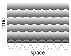
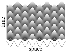
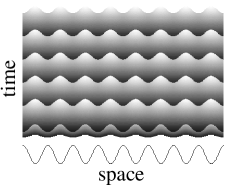
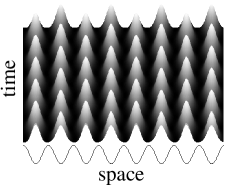
Figure 6: The left column shows harmonic solutions for the fields $w_{2}^{h}$ (top) and $v=\hat{v}_{0}+w_{2}^{h}$ (bottom) and the right column subharmonic solutions for the same fields, i.e. $w_{2}^{sh}$ (top) and $v=\hat{v}_{0}+w_{2}^{sh}$ (bottom). Solid lines indicate the spatial modulation $M(x)$. The illumination is given by $\phi_{0}=1.42$ and the forcing amplitude by $G=0.025$ in part (a) and by $G=0.15$ in part (b). Further parameters are $a=12,c=0.55,\sigma=5,d=0.8,k=0.2$. The parameter values in the $\phi_{0}-G$ plane are marked by crosses in Fig. 4(b).

The solution $w_{2}^{h}(x,t)$ describes spatially modulated oscillations whose spatial profile becomes more pronounced when the basic solution $\hat{v}_{0}$ is included. The time evolution of the field $w_{2}^{sh}$ resembles that of a standing wave with twice the wavelength of the forcing and, indeed, it is well described by a superposition of three standing waves $w_{2}^{sh}(x,t)=\sum_{j=1}^{3}B_{j}\sin{(\omega_{c}^{sh}t+\varphi_{j})}\sin{[(2j-1)kx]}$ with real amplitudes $B_{j}$ and phases $\varphi_{j}$. On the bottom right the full solution $v=\hat{v}_{0}+w_{2}^{sh}$ of the Lengyel-Epstein model is shown. Note, the basic solutions $\hat{v}_{0},~{}\hat{u}_{0}$ have the same periodicity as the spatial modulation. The nonlinear solutions for the other fields $w_{1}$ and $u=\hat{u}_{0}+w_{1}$ look very much like the ones shown in Fig. 6 and they are therefore not presented here. Starting the simulations with spatially subharmonic states and decreasing the illumination $\phi_{0}$ continuously, the subharmonic pattern is stable against small perturbations up to the dotted line in Fig. 4(a). On exceeding this border line, the subharmonic solution becomes unstable and spatially harmonic patterns emerge.

Close to the threshold of the Hopf bifurcation, where the amplitude of the oscillations is small, the dynamics of the Lengyel-Epstein model may be described by a so-called amplitude equation as discussed in the next section.

V Amplitude equation

Below the critical value $\phi_{0c}$ of the control parameter $\phi_{0}$, the basic state $\mathbf{u}_{0}=(u_{0},v_{0})$ of the Lengyel-Epstein model (1) becomes linearly unstable against small oscillatory perturbations $\mathbf{u}_{1}$ as described in Sec. III.1. The magnitude of $\mathbf{u}_{1}$ beyond threshold is restricted by nonlinear terms in $\mathbf{u}_{1}$ which are of cubic order for a supercritical bifurcation. In this case one may derive a universal amplitude equation for the slowly varying amplitude $A(x,t)$ in order to describe the dynamics close to the threshold CrossHo . The technique for this derivation is a multiple scale analysis where the full solution $\mathbf{u}_{1}$ is decomposed into a fast varying oscillation $\propto\exp{(i\omega_{c}t)}$ with the frequency $\omega_{c}$ and a spatially and temporally slowly varying amplitude $A(x,t)$: $\mathbf{u}_{1}=A(x,t)\mathbf{u}_{e}\exp{(i\omega_{c}t)}+{\rm c.c.}$.

The usage of amplitude equations is a well established method to characterize the universal properties of a pattern at small amplitudes close to its threshold. A particularly well-known amplitude equation is found for a spatially homogeneous Hopf bifurcation, which has been investigated very intensively over the recent decades and a recent review of this subject is given by Ref. Aranson:02.1 .

For the derivation of the amplitude equation one introduces as an expansion parameter the small distance to the threshold $\varepsilon=\frac{\phi_{0c}-\phi_{0}}{\phi_{0c}}$ and the expansion holds in the range $A\propto\varepsilon^{1/2}$. Here we assume additionally that the modulation $M(x)$ is also of the order $\varepsilon$. For this case we generalize the amplitude equation for an oscillatory bifurcation by including the spatial modulation $M(x)$:

$$\tau_{0}\partial_{t}A = \varepsilon\left(1+ic_{1}\right)A+\xi_{0}^{2}\left(1+ib\right)\partial_{x}^{2}A$$

$$+s_{1}\left(1+is_{2}\right)MA-g\left(1+ic_{2}\right)\mid A\mid^{2}A\,.$$

An explicit derivation of this equation from the basic Eqs. (1) is given in the Appendix and a special case of it is given in Ref. Zimmermann:96.2 . All coefficients in Eq. (V) describe physical quantities, such as the relaxation time $\tau_{0}$, the linear and nonlinear frequency shift $c_{1}$ and $c_{2}$, respectively, the coherence length $\xi_{0}$ and the linear frequency dispersion $\xi_{0}^{2}b$. For $g>0$ the bifurcation is supercritical and otherwise subcritical. The analytical expressions for all these coefficients in terms of the parameters of the basic equations (1) are rather lengthy and, instead of giving their analytical forms, we have plotted them in Fig. 7 as functions of the parameter $c$ and for three different values of $a$.

It is worthwhile mentioning that apart from the coefficients $s_{1}$ and $s_{2}$, all the other linear coefficients can be calculated from the dispersion relation $\lambda(\phi_{0},q^{2},\ldots)={\rm Re}(\lambda)\pm i{\rm Im}(\lambda)$ of the Lengyel-Epstein model given in Eq. (15) by the following expressions CrossHo ; Zimmermann:93.1

$$\tau_{0} =\frac{1}{\phi_{0c}\partial{\rm Re}(\lambda)/\partial\phi_{0}}~{}, c_{1} =\phi_{0c}\tau_{0}\,\frac{\partial\omega}{\partial\phi_{0}}\,,$$ (35a)

$$\xi_{0}^{2} =\frac{1}{2\phi_{0c}}\frac{\partial^{2}\phi_{0}}{\partial q^{2}}~{}, b =-\frac{\tau_{0}}{2\xi_{0}^{2}}\frac{\partial^{2}\omega}{\partial q^{2}}~{}.$$ (35b)

Here $\omega={\rm Im}(\lambda)$ and the derivatives are evaluated at the critical values $\phi_{0c},q_{c},\omega_{c}$. For a vanishing modulation these coefficients describe the linear properties of the Lengyel-Epstein model near threshold. It is however indispensable to carry out the perturbation expansion in order to determine the linear coefficients $s_{1}$ and $s_{2}$ as well as the nonlinear coefficients $g$ and $c_{2}$ as functions of the parameters of the basic equations.

The term $i\varepsilon c_{1}A$ in Eq. (V) can be removed by the transformation $\widetilde{A}=e^{-i\varepsilon c_{1}t}A$. For convenience we can scale out the coefficients $\tau_{0},\xi_{0},s_{1},g$ by a suitable choice of time, space and amplitude scales

$$t^{\prime} =t/\tau_{0}\,, x^{\prime} =x/\xi_{0}\,,$$

$$A^{\prime} =g^{1/2}A\,, G^{\prime} =s_{1}G\,,$$ (36)

and one obtains the following rescaled amplitude equation:

$$\partial_{t}A = \varepsilon A+\left(1+ib\right)\partial_{x}^{2}A+\left(1+is_{2}\right)MA$$ (37)

$$-\left(1+ic_{2}\right)\mid A\mid^{2}A\,,$$

where we have kept for simplicity the same symbols for the scaled quantities. The amplitude equation is invariant under an arbitrary phase transformation as $A\rightarrow A\exp{(i\psi)}$.

Figure 7: The coefficients of the amplitude equation (V) are plotted as functions of the parameter $c$ of the Lengyel-Epstein model and for three different values $a$: $a=14$ (solid lines), $a=12$ (dashed lines) and $a=10$ (dotted lines). The critical illumination $\phi_{0c}$ and the Hopf frequency $\omega_{c}$ along these curves are shown in Fig. 2. Further parameters are $\sigma=5,d=1$.

V.1 Determination of the threshold

We investigate in this section how the spatial modulation $M(x)$ changes the bifurcation scenario from the basic state $A=0$ of Eq. (37) into a spatial pattern. In the absence of the modulation, i.e. $G=0$, the linear part of Eq. (37) is solved by $A=Fe^{\lambda t+iqx}$ and this ansatz leads in the neutrally stable case ${\rm Re}(\lambda)=0$ to an expression for the neutral curve $\varepsilon_{0}(q)$ and the frequency dispersion $\omega_{0}(q)={\rm Im}(\lambda)$,

$$\varepsilon_{0}(q) =q^{2}\,, \omega_{0}(q) =-bq^{2}\,\,.$$ (38)

Minimizing $\varepsilon_{0}(q)$ determines the threshold $\varepsilon_{c}=0$, the critical wave number $q_{c}=0$ and the frequency $\omega_{c}=0$. In the presence of $M(x)$ the bifurcation properties of Eq. (37) are changed, as illustrated in the following by a perturbation calculation for small modulation amplitudes.

V.1.1 Perturbation method for small amplitudes of $M(x)$

For small forcing amplitudes $G\ll 1$ we introduce a small expansion parameter $\eta\ll 1$ with $M(x)=\eta{\bar{M}}(x)$. Since the amplitude equation (37) is of first order with respect to time, the solution of its linear part has an exponential time dependence and for small values of the modulation amplitude, $G=\eta{\bar{G}}$, the linear solution may be expanded in powers of the modulation strength $\eta$

$$A=e^{\lambda t}\left(A_{0}+\eta A_{1}+\eta^{2}A_{2}+\cdots\right)\,.$$ (39)

Applying the neutral stability condition ${\rm Re}(\lambda)=0$, the perturbation in Eq. (39) does neither grow nor decay, which separates the parameter regime where the basic state $A=0$ is stable from the range where $A=0$ is unstable.

The threshold is shifted due to the modulation and therefore, the control parameter $\varepsilon_{c}$ and the frequency $\omega_{c}={\rm Im}(\lambda)$ are also expanded with respect to $\eta$

$$\varepsilon_{c} = \varepsilon_{c}^{({0})}+\eta\varepsilon_{c}^{({1})}+\eta^{2}\varepsilon_{c}^{({2})}+\cdots\,\,,$$ (40a)

$$\omega_{c} = \omega_{c}^{(0)}+\eta\omega_{c}^{(1)}+\eta^{2}\omega_{c}^{(2)}+\cdots\,\,.$$ (40b)

The expansions given in Eqs. (39) and (40) provide the following hierarchy of equations defining the neutral stability of the basic state $A=0$:

$$\eta^{0}:\,\,\,{\cal L}_{0}A_{0} =0\,,$$ (41a)

$$\eta^{1}:\,\,\,{\cal L}_{0}A_{1} =[\varepsilon_{c}^{({1})}+i\omega_{c}^{(1)}+(1+is_{2}){\bar{M}}]A_{0}\,,$$ (41b)

$$\eta^{2}:\,\,\,{\cal L}_{0}A_{2} =[\varepsilon_{c}^{({1})}+i\omega_{c}^{(1)}+(1+is_{2}){\bar{M}}]A_{1}$$

$$+[\varepsilon_{c}^{({2})}+i\omega_{c}^{(2)}]A_{0}\,,$$ (41c)

with the linear operator ${\cal L}_{0}=\partial_{t}-i\omega_{c}^{(0)}-\varepsilon_{c}^{({0})}-(1+ib)\partial_{x}^{2}$. These equations may be solved by a spatial dependence which is either harmonic

$$A_{0} =F_{0}\,,$$ (42a)

$$A_{1} =F_{2}e^{2ikx}+F_{-2}e^{-2ikx}\,,$$ (42b)

$$\cdots$$

or subharmonic

$$A_{0} =F_{1}e^{ikx}+F_{-1}e^{-ikx}\,,$$ (42c)

$$A_{1} =F_{3}e^{3ikx}+F_{-3}e^{-3ikx}\,,$$ (42d)

$$\cdots$$

with respect to $M(x)$. In order to distinguish between the harmonic and subharmonic results we introduce $\varepsilon_{h},\omega_{h}$ for the harmonic case and $\varepsilon_{sh},\omega_{sh}$ for the subharmonic one. From a solubility condition on the right hand side of Eqs. (41b) and (41) the corrections to $\varepsilon_{c}$ and $\omega_{c}$ may be calculated. The solution $A_{1}$ of Eq. (41b) is given for the harmonic ansatz by

$$A_{1}=\frac{G(1+is_{2})F_{0}}{4k^{2}(1+ib)}\left(e^{2ikx}+e^{-2ikx}\right),$$ (43)

and in the case of the subharmonic ansatz by

$$A_{1}=\frac{G(1+is_{2})}{8k^{2}(1+ib)}\left(F_{1}e^{3ikx}+F_{-1}e^{-3ikx}\right),$$ (44)

whereas the solution $A_{2}$ of Eq. (41) is not needed explicitly to determine the corrections $\varepsilon_{c}^{({2})}$ and $\omega_{c}^{(2)}$, respectively. The expansions of the threshold $\varepsilon_{c}$ and the frequency $\omega_{c}$ up to order $O(\eta^{2})$ are given for the harmonic case by

$$\varepsilon_{h} =-\eta^{2}\frac{{\bar{G}}^{2}(1-s_{2}^{2}+2bs_{2})}{2k^{2}(1+b^{2})}\,,$$ (45a)

$$\omega_{h} =\eta^{2}\frac{{\bar{G}}^{2}\left[b(1-s_{2}^{2})-2s_{2}\right]}{2k^{2}(1+b^{2})}\,,$$ (45b)

and for the subharmonic case by

$$\varepsilon_{sh} =k^{2}-\eta{\bar{G}}-\eta^{2}\frac{{\bar{G}}^{2}(1-s_{2}^{2}+2bs_{2})}{8k^{2}(1+b^{2})}\,,$$ (46a)

$$\omega_{sh} =bk^{2}-\eta s_{2}{\bar{G}}+\eta^{2}\frac{{\bar{G}}^{2}\left[b(1-s_{2}^{2})-2s_{2}\right]}{8k^{2}(1+b^{2})}\,.$$ (46b)

If one increases the control parameter in Eq. (37) from below, the lowest of the two thresholds $\varepsilon_{h}$ and $\varepsilon_{sh}$ determines whether the basic state $A=0$ is unstable against spatially harmonic solutions, i.e. if $\varepsilon_{h}<\varepsilon_{sh}$, or spatially subharmonic solutions, i.e. if $\varepsilon_{sh}<\varepsilon_{h}$. By replacing $k\to\xi_{0}k$ and ${\bar{G}}\to s_{1}{\bar{G}}$ in the expressions (45) and (46), the thresholds $\varepsilon_{h,sh}$ and the frequencies $\omega_{h,sh}$ for the amplitude equation (V) follow.

V.1.2 Numerical determination of the threshold

Because of the periodically varying coefficient $M(x)$ in Eq. (37), the general linear solution may be represented, similar as in Sec. III.3, by a Floquet-Bloch expansion

$$A(x,t)=e^{\lambda t+iqx}\sum_{j=-N}^{N}F_{j}e^{ij2kx}\quad\left({\rm with}\,\,0\leq q<2k\right),$$ (47)

up to an appropriate number $N$. Without spatial forcing all coefficients but $F_{0}$ vanish. The perturbation in Eq. (47) grows for a chosen parameter combination if ${\rm Re}(\lambda)>0$ and it decays if ${\rm Re}(\lambda)<0$. We are again primarily interested in the neutrally stable case ${\rm Re}(\lambda)=0$, separating the stable from the unstable regime. After inserting the ansatz for $A$ into the linear part of Eq. (37), the explicit $x$-dependence is removed by multiplying the equation with $\exp{(-il2kx)}$ ($l=-N,\ldots,N$) and integrating with respect to $x$. From this procedure the eigenvalue problem

$$\mathcal{A}\vec{F}=\rho\vec{F}\qquad\left[\vec{F}=(F_{-N},\ldots,F_{N})\right]$$ (48)

follows, where the matrix $\mathcal{A}$ is a band matrix of width $(2N+1)$ with the coefficients

$$\mathcal{A}_{l,l} = (1+ib)(q+2lk)^{2}\,,$$ (49a)

$$\mathcal{A}_{l,l-2} = -(1+is_{2})G\,,$$ (49b)

$$\mathcal{A}_{l,l+2} = \mathcal{A}_{l,l-2}\,.$$ (49c)

From a solvability condition for the homogeneous system of equations (48),

$${\rm det}(\mathcal{A}-\rho\mathcal{I})=f(G,k,q\ldots)=0\,,$$ (50)

$(\mathcal{I}$ is the unity matrix) the eigenvalues $\rho_{i}$ are determined as functions of the parameters and they can be sorted in ascending order with respect to their real parts ${\rm Re}(\rho_{i})$. Keeping all parameters besides $q$ fixed, the neutral curve $\varepsilon_{0}(q)$ and the frequency $\omega_{0}(q)$ can be determined from the eigenvalue with the lowest real part $\widehat{\rho}={\rm min}[{\rm Re}(\rho_{i})]$. Minimizing $\varepsilon_{0}(q)$ gives then the threshold $\varepsilon_{c}$, the critical wave number $q_{c}$ and the critical frequency $\omega_{c}=\omega_{0}(q=q_{c})$. In this way, we found that the minimum of the neutral curve is either given at $q_{c}=0$ determining the harmonic threshold $\varepsilon_{h}$, or at $q_{c}=k$ determining the subharmonic threshold $\varepsilon_{sh}$. The harmonic and subharmonic contributions of the ansatz in Eq. (47) with respect to $M(x)$ separate for the linear part of Eq. (37), and the two thresholds $\varepsilon_{h}$ and $\varepsilon_{sh}$ may be calculated independently.

In order to obtain the analogous eigenvalue equation with respect to the unscaled amplitude equation given in Eq. (V), one has to replace in Eqs. (49) the wave numbers $q$ and $k$ by $\xi_{0}q$ and $\xi_{0}k$, respectively, as well as the amplitude $G$ by $s_{1}G$.

V.2 Results

One interesting question is the location of the boarder separating the parameter range where the harmonic pattern is preferred at threshold from that range where the subharmonic pattern is favored, whereby the borderline is determined by the condition $\varepsilon_{h}=\varepsilon_{sh}$. In terms of our perturbational results as given in Sec. V.1.1 this condition leads to a second order polynomial in the modulation amplitude $G$ with its two solutions

$$G_{\pm} = \frac{4k^{2}(1+b^{2})}{3(1-s_{2}^{2}+2bs_{2})}\pm\frac{2k^{2}(1+b^{2})}{3(1-s_{2}^{2}+2bs_{2})}$$ (51)

$$\times\sqrt{4-6\frac{1-s_{2}^{2}+2bs_{2}}{1+b^{2}}}\,\,.$$

There is a finite range in $G$ where subharmonic solutions are preferred, namely if the following inequality

$$4\left(1+b^{2}\right)-6\left(1-s_{2}^{2}+2bs_{2}\right)>0\,$$ (52)

is fulfilled.

Figure 8: The two solutions $G_{+}$ (solid lines) and $G_{-}$ (dotted lines), as given by Eq. (51), are shown as a function of the coefficient $s_{2}$ and for the parameters $k=0.25,b=1.5$. The areas with pure harmonic and subharmonic solutions at threshold are marked by h and s, respectively.

The harmonic threshold is the lowest one for modulation amplitudes $G<G_{-}$ and $G>G_{+}$. In the finite range $G_{-}<G<G_{+}$ the subharmonic threshold $\varepsilon_{sh}$ drops below the harmonic one. The two amplitudes $G_{+}$ and $G_{-}$ according to the formula (51) are plotted in Fig. 8 as functions of the coefficient $s_{2}$. The ranges in which subharmonic or harmonic solutions are preferred are marked by s and h, respectively.

In the parameter range $s_{2}>b+\sqrt{1+b^{2}}$ and $s_{2}<b-\sqrt{1+b^{2}}$ the harmonic threshold has a positive curvature as a function of $G$, $\partial^{2}\varepsilon_{h}/\partial G^{2}>0$, which can be readily verified from Eq. (45a). Consequently, at small values of $G$ the threshold $\varepsilon_{h}$ is shifted upwards while the subharmonic threshold is dominated by the linear decrease $\varepsilon_{sh}\propto k^{2}-G$. These trends of the two thresholds apparently promote the appearance of subharmonic patterns.

Figure 9: The harmonic (solid lines) and subharmonic (dashed lines) threshold as well as the corresponding frequencies are plotted as functions of the forcing amplitude $G$ for two sets of parameters, in part (a) for $k=0.25,~{}b=5,~{}s_{2}=0.5$ and in part (b) for $k=0.25,~{}b=0.01,~{}s_{2}=3$. In order to generate the numerical results $N=32$ modes in the Floquet expansion (47) have been used. Subharmonic patterns occur in the $G$-range where $\varepsilon_{sh}<\varepsilon_{h}$. The second point of intersection between the harmonic and subharmonic branch is located at $G\simeq 1.53$ in part (a) and at $G\simeq 0.12$ in part (b). For comparison, the symbols in part (a) are obtained by the analytical expressions given in Eqs. (45) and (46).

For arbitrary values of the modulation amplitude $G$ and wave number $k$ the linear stability of the basic state $A=0$ of Eq. (37) has to be determined numerically by solving the eigenvalue problem (48). The harmonic threshold $\varepsilon_{h}$ and the subharmonic threshold $\varepsilon_{sh}$ are calculated separately and some results for them as well as for the corresponding critical frequencies $\omega_{h}$ and $\omega_{sh}$, respectively, are shown in Fig. 9 for two sets of parameters. The harmonic branches $\varepsilon_{h},\omega_{h}$ (solid lines) and subharmonic branches $\varepsilon_{sh},\omega_{sh}$ (dashed lines) have been calculated for $N=32$ Fourier modes, which has been proven to be a reasonable approximation. The symbols in part (a) indicate the results of the perturbation calculation as given in Eqs. (45) and (46), which are in good agreement with the numerical results for small forcing amplitudes $G$. The points of intersection between the branches $\varepsilon_{h}$ and $\varepsilon_{sh}$ are roughly given by $G_{-}\simeq 0.068$, $G_{+}\simeq 1.53$ in part (a) and by $G_{-}\simeq 0.028$, $G_{+}\simeq 0.12$ in part (b). For comparison, the perturbation calculation yields $G_{-}\simeq 0.068$, $G_{+}\simeq 0.68$ for the parameters in part (a) and $G_{-}\simeq-0.048$, $G_{+}\simeq 0.027$ for the ones in part (b). As mentioned above, the sign of the curvature $\partial^{2}\varepsilon_{h}/\partial G^{2}$ at small amplitudes $G$ may be changed by varying the coefficients $b$ and $s_{2}$, which can be recognized by comparing the course of $\varepsilon_{h}$ in part (a) given for $(b,s_{2})=(5,0.5)$ and in part (b) given for $(b,s_{2})=(0.01,3)$.

Harmonic solutions are preferred for large modulation wave numbers $k$, and in the limiting case $k\to\infty$, the harmonic threshold approaches $\varepsilon_{h}=0$ while the subharmonic threshold diverges in this limit, being in agreement with the expressions given in Eqs. (45a) and (46a). In the opposite limit, i.e. $k\to 0$, the thresholds $\varepsilon_{h}$ and $\varepsilon_{sh}$ tend to $\varepsilon_{h,sh}=-2G$, which has to be computed numerically. We remind the reader that the thresholds $\phi_{0c}^{h}(k)$ and $\phi_{0c}^{sh}(k)$, as obtained for the Lengyel-Epstein model, exhibit qualitatively the same behavior as a function of $k$, cf. Fig. 5(a).

In Fig. 10 the harmonic threshold $\varepsilon_{h}$ (solid line) and the subharmonic threshold $\varepsilon_{sh}$ (dashed line) are plotted as functions of the linear coefficient $s_{2}$ (top) and $b$ (bottom). For large values of the modulus $|s_{2}|$ the subharmonic threshold drops below the harmonic one and spatially subharmonic solutions appear at threshold of the Hopf bifurcation. Regions solely supporting harmonic or subharmonic patterns are found in the range s and h, respectively. The points of intersection between both thresholds are roughly given by $s_{2}\simeq\pm 2$. For comparison, $s_{2}\simeq\pm 1.84$ is obtained from the perturbation calculation. According to the bottom part of the figure, subharmonic solutions are preferred in a finite range of the parameter $b$ similar as the $G$-range in Fig. 9. Again, within the regions marked by s and h only subharmonic or harmonic patterns are found.

From the inequality given in Eq. (52) one may easily deduce the following limiting cases. For $b=0$ subharmonic solutions are favored in the range $s_{2}^{2}>1/3$ and for $s_{2}=0$ in the range $b^{2}>1/2$, while $b=s_{2}=0$ seems to lead to a contradiction. Therefore, one of the two linear coefficients $b$ and $s_{2}$ is necessary for the occurrence of spatially subharmonic patterns.

Figure 10: The dependence of the harmonic (solid line) and subharmonic (dashed line) threshold on the coefficient $s_{2}$ is shown in the top part for a set of parameters given by $G=0.04,~{}k=0.25,~{}b=0.01$. The bottom part shows both thresholds as function of the coefficient $b$ and for the parameters $G=0.05,~{}k=0.24,~{}s_{2}=3$. The range where harmonic solutions are preferred is marked by h and that of subharmonic ones by s.

V.2.1 Comparison with the Lengyel-Epstein model

In order to be able to compare directly the results for the harmonic and subharmonic thresholds with those obtained from the basic equations (1), we have to consider the linear part of the unscaled amplitude equation (V), which reflects the typical length scale, $\xi_{0}$, time scale, $\tau_{0}$, and amplitude scale, $s_{1}$, of the Lengyel-Epstein model. In this context one may raise the question under which conditions are the thresholds $\varepsilon_{h},\varepsilon_{sh}$ determined by the amplitude-equation approach, and the thresholds $\phi_{0c}^{h},\phi_{0c}^{sh}$ determined by the Lengyel-Epstein model, in (good) agreement? Such a comparison of the thresholds, e.g. as a function of the modulation amplitude $G$, gives also some insights into the validity range of the amplitude equation which is a priori unknown.

For this comparison, we have to replace in the eigenvalue problem in Eq. (48) the wave numbers $q$ and $k$ by $\xi_{0}q$ and $\xi_{0}k$ as well as the amplitude $G$ by $s_{1}G$. Furthermore, the values of the linear coefficients $\tau_{0},c_{1},\xi_{0},b,s_{1}$ and $s_{2}$ are determined by the parameters of the Lengyel-Epstein model as shown, for instance, in Fig. 7.

Figure 11 shows the harmonic threshold (triangles) and the subharmonic one (squares) as given for the Lengyel-Epstein model as well as the related thresholds obtained from the amplitude equation (lines). The latter ones are calculated with respect to the illumination rate by using the formula $\phi_{0c}=\phi_{0c}(G=0)(1-\varepsilon_{c})$. According to this figure, one finds a qualitatively similar behavior of the associated thresholds. For comparison, the relative error between the harmonic thresholds is roughly given by $5\%$ and between the subharmonic thresholds by $6\%$ calculated for $G=0.06$. These deviations become smaller for decreasing values of the wave numbers $k$ or by decreasing the modulation amplitude $G$. Moreover, the finite $G$-range in which the subharmonic solution has the higher threshold is also in good agreement with the range given by the amplitude approach.

Figure 11: Comparison between the harmonic (h) and subharmonic (s) thresholds, which have been calculated for the Lengyel-Epstein model (symbols) by solving the eigenvalue equation (31) and for the amplitude equation (lines) by solving the eigenvalue equation (48). For the latter one, we have replaced the wave numbers $q$ and $k$ by $\xi_{0}q$ and $\xi_{0}k$ as well as the amplitude $G$ by $s_{1}G$. The modulation wave number is $k=0.05$. The other parameters are given by $a=10,c=0.55,\sigma=5,d=1$ leading to the coefficients of the amplitude equation (V) as given in Fig. 7 (dotted line).

Another interesting comparison between both models is the change of the sign of the curvature of the harmonic threshold, which has been found for the amplitude equation, cf. Eq. (45a). This significant behavior of the threshold has also been observed for the Lengyel-Epstein model in a parameter regime determined by the amplitude equation. If the curvature of $\phi_{0c}^{h}(G)$ is positive the Hopf bifurcation also occurs for larger illuminations $\phi_{0}$, being in contrast to the situation shown in Fig. 4(a) or Fig. 11.

VI Summary and conclusions

We have investigated the effects of a spatially periodic modulated control parameter on an oscillating chemical reaction described by the Lengyel-Epstein model. This reaction exhibits a supercritical Hopf bifurcation and it provides due to its photosensitivity a simple approach to study the response of the reaction with respect to a spatially modulated illumination.

We find that in the range of intermediate values of the modulation amplitude $G$ the bifurcation to the oscillatory chemical reaction is subharmonic with respect to the external modulation whereas for small and large modulation amplitudes the bifurcation is harmonic. Beyond the bifurcation point the subharmonic solution is preferred in a finite range of the control parameter before a transition to the harmonic pattern takes place at larger values. The related results of the stability calculations of the basic state with respect to small perturbations are summarized in Figs. 4 and 5.

Close to the threshold of the Hopf bifurcation, an amplitude equation is presented which is an extension of the well-known complex Ginzburg-Landau equation for spatially homogeneous, oscillatory bifurcations. This equation is generic for oscillatory systems near threshold underlying a spatially varying control parameter and it may therefore also be found for other systems having the same symmetry properties as the considered Lengyel-Epstein model.

The stability limit of the basic state of the amplitude equation has been determined by a perturbation calculation and by solving the general linear problem numerically. Good agreement of the two approaches is found for small forcing amplitudes. It has been shown that intermediate forcing amplitudes lead also to subharmonic solutions, while weak and strong forcing amplitudes favor harmonic solutions. A rough estimation of the validity range of the amplitude equation has been given by comparing the harmonic and subharmonic thresholds with those obtained for the Lengyel-Epstein model itself. We have found that the amplitude equation describes the linear properties of the Lengyel-Epstein model to a great extent for long-wavelength modulations and small forcing amplitudes.

According to our results we expect in experiments on chemical reactions, which are described by the Lengyel-Epstein model, also a transition to subharmonic patterns induced by a spatially periodic illumination.

Instead of considering stationary forcing, the effect of spatiotemporal forcing on an oscillating chemical system may also be investigated. Here, the forcing has the form of a traveling wave similar as introduced recently to study the effects of spatiotemporal forcing on stationary Turing patterns Sagues:2004.1 ; Sagues:2003.1 as well as on oblique stripe patterns in anisotropic systems Schuler:2004.1 . This special type of forcing breaks a further symmetry of the system, the reflection symmetry, which may induce a more complex spatiotemporal behavior to which forthcoming work is devoted.

*

Appendix A Scheme for the derivation of the amplitude equation

For the derivation of the amplitude equation (V), a small reduced control parameter is introduced,

$$\varepsilon=\frac{\phi_{0c}-\phi_{0}}{\phi_{0c}}\,\,,$$ (53)

which is a measure for the distance from the threshold of the Hopf bifurcation. At threshold the linear solutions of the Lengyel-Epstein model may be written as

$$\mathbf{u}_{1}=A\mathbf{u}_{e}\,e^{i\omega_{c}t}+{\rm c.c.}\,,$$ (54)

where $A$ describes the common amplitude of the two fields $u_{1},v_{1}$ and the eigenvector $\mathbf{u}_{e}=(1,E_{0})^{T}$ describes their amplitude ratio, cf. Eq. (13).

For the perturbation expansion we introduce slow time and space variables CrossHo

$$X =\varepsilon^{1/2}x\,, T_{1} =\varepsilon^{1/2}t\,, T =\varepsilon t\,$$ (55)

and the solution $\mathbf{u}_{1}$ may be written as a product of a slowly varying amplitude and a fast oscillating exponential function

$$\mathbf{u}_{1}=A(X,T,T_{1})\mathbf{u}_{e}\,e^{i\omega_{c}t}+{\rm c.c.}\,.$$ (56)

According to the chain rule one may replace time and space derivatives by the following expressions

$$\partial_{t} \to\partial_{t}+\varepsilon^{1/2}\partial_{T_{1}}+\varepsilon\partial_{T}\,, \partial_{x} \to\partial_{x}+\varepsilon^{1/2}\partial_{X}\,.$$ (57)

Note that $\partial_{t}$ and $\partial_{x}$ on the right-hand side only act on the rapid dependences. We further assume small modulation amplitudes $M(x)=\varepsilon{\bar{M}}(x)$ with ${\bar{M}}(x)\propto O(1)$ and wave numbers $k=\varepsilon^{1/2}{\bar{k}}$ with ${\bar{k}}\propto O(1)$. An attribute of the $\pm$ symmetry of a supercritical oscillatory bifurcation is the power law for the oscillation amplitude $A\sim\sqrt{\varepsilon}$. Accordingly, the solutions of the basic equation (7) are expanded near threshold with respect to powers of $\varepsilon^{1/2}$,

$$\mathbf{u}=\mathbf{u}_{0}+\varepsilon^{1/2}\mathbf{u}_{1}+\varepsilon\mathbf{u}_{2}+\varepsilon^{3/2}\mathbf{u}_{3}+\cdots\,\,.$$ (58)

The components of $\mathbf{u}_{0}$ describe the stationary solutions as given in Eq. (8) and the components of $\mathbf{u}_{1}=A_{1}\mathbf{u}_{e}\exp{(i\omega_{c}t)}+{\rm c.c.}$ provide the linear oscillatory solutions at threshold as discussed in Sec. III.1. Note that the amplitude $A_{1}$ and the amplitude $A$ in Eq. (56) only differ by a factor of $\varepsilon^{1/2}$. The expansions for $\mathcal{L},\mathbf{N}$ and $\mathbf{V}$ in Eq. (7) are given by

$$\mathcal{L} = \mathcal{L}_{0}+\varepsilon^{1/2}\mathcal{L}_{1}+\varepsilon\mathcal{L}_{2}\,\,,$$ (59a)

$$\mathbf{N} = \mathbf{N}_{0}+\mathbf{L}+\varepsilon\mathbf{N}_{2}+\varepsilon^{3/2}\mathbf{N}_{3}+\cdots\,\,,$$ (59b)

$${\rm with}\quad\mathbf{L} = \varepsilon^{1/2}\mathcal{M}_{0}\mathbf{u}_{1}+\varepsilon\mathcal{M}_{0}\mathbf{u}_{2}+\varepsilon^{3/2}\mathcal{M}_{0}\mathbf{u}_{3}+\cdots\,\,,$$

$$\mathbf{V} = \mathbf{V}_{0}+\varepsilon\mathbf{V}_{2}\,\,,$$ (59c)

and with the explicit expressions of the linear operators ${\mathcal{L}}_{0},{\mathcal{L}}_{1}$ as well as ${\mathcal{L}}_{2}$:

$${\mathcal{L}}_{0} =\begin{pmatrix}\partial_{t}+c&0\\ -\sigma c&\partial_{t}\end{pmatrix},$$

$${\mathcal{L}}_{1} =\begin{pmatrix}\partial_{T_{1}}-2\partial_{x}\partial_{X}&0\\ 0&\partial_{T_{1}}-2\sigma d\partial_{x}\partial_{X}\end{pmatrix},$$

$${\mathcal{L}}_{2} =\begin{pmatrix}\partial_{T}-\partial_{X}^{2}&0\\ 0&\partial_{T}-\sigma d\partial_{X}^{2}\end{pmatrix}.$$ (60)

The nonlinear vectors in the expansions (59b) and (59c) are given by

$${\mathbf{N}}_{0} = \frac{u_{0}v_{0}}{1+u_{0}^{2}}\begin{pmatrix}-4\\ -\sigma\end{pmatrix},$$

$${\mathbf{N}}_{2} = -\begin{pmatrix}4\\ \sigma\end{pmatrix}\left(E_{1}u_{1}v_{1}+E_{2}u_{1}^{2}\right),$$

$${\mathbf{N}}_{3} = -\begin{pmatrix}4\\ \sigma\end{pmatrix}{\cal N}_{3}~{},\qquad{\rm with}$$

$${\cal N}_{3} = \left[R_{1}(u_{1}v_{2}+u_{2}v_{1})+R_{2}u_{1}u_{2}+R_{3}v_{1}u_{1}^{2}+R_{4}u_{1}^{3}\right]$$

and

$${\mathbf{V}}_{0}=\begin{pmatrix}a-\phi_{0c}\\ \sigma\phi_{0c}\end{pmatrix},\quad{\mathbf{V}}_{2}=\begin{pmatrix}\phi_{0c}-{\bar{M}}\\ -\sigma\phi_{0c}+\sigma{\bar{M}}\end{pmatrix},$$ (61)

where the abbreviations

$$E_{1} =\frac{1-u_{0}^{4}}{\left(1+u_{0}^{2}\right)^{3}}\,, E_{2} =\frac{v_{0}\left(u_{0}^{3}-3u_{0}\right)}{\left(1+u_{0}^{2}\right)^{3}}\,,$$

$$R_{1} =\frac{1+u_{0}^{2}-u_{0}^{4}-u_{0}^{6}}{\left(1+u_{0}^{2}\right)^{4}}\,, R_{2} =\frac{-2u_{0}v_{0}\left(3+2u_{0}^{2}-u_{0}^{4}\right)}{\left(1+u_{0}^{2}\right)^{4}}\,,$$ (62)

$$R_{3} =\frac{u_{0}^{5}-3u_{0}-2u_{0}^{3}}{\left(1+u_{0}^{2}\right)^{4}}\,, R_{4} =\frac{6u_{0}^{2}v_{0}-u_{0}^{4}v_{0}-v_{0}}{\left(1+u_{0}^{2}\right)^{4}}\,,$$

have been introduced. Inserting all expressions into Eq. (7) yields at successive orders of $\varepsilon^{1/2}$

$$\varepsilon^{0}:\,\,\,{\mathcal{L}}_{0}\mathbf{u}_{0} =\mathbf{N}_{0}+\mathbf{V}_{0}\,,$$ (63a)

$$\varepsilon^{1/2}:\,\,\,{\mathcal{L}}_{0}\mathbf{u}_{1} ={\mathcal{M}}_{0}\mathbf{u}_{1}\,,$$ (63b)

$$\varepsilon^{1}:\,\,\,{\mathcal{L}}_{0}\mathbf{u}_{2} ={\mathcal{M}}_{0}\mathbf{u}_{2}-{\mathcal{L}}_{1}\mathbf{u}_{1}+\mathbf{N}_{2}+\mathbf{V}_{2}\,,$$ (63c)

$$\varepsilon^{3/2}:\,\,\,{\mathcal{L}}_{0}\mathbf{u}_{3} ={\mathcal{M}}_{0}\mathbf{u}_{3}+\mathbf{N}_{3}-{\mathcal{L}}_{2}\mathbf{u}_{1}\,,$$ (63d)

$$\cdots\,\,.$$

Equation (63a) determines the basic state as given by Eq. (8) while Eq. (63b) reproduces the threshold condition (14) with the solution known already from Eq. (15). Since $\left({\mathcal{L}}_{0}-{\mathcal{M}}_{0}\right)\mathbf{u}_{1}=\mathbf{0}$ holds due to Eq. (63b), the contribution ${\mathcal{L}}_{1}\mathbf{u}_{1}$ on the right-hand side of Eq. (63c) has to vanish leading to the constraint $\partial_{T_{1}}A_{1}=0$. In order to solve the inhomogeneous equation (63c), we choose the following ansatz:

$$\mathbf{u}_{2}=\begin{pmatrix}u_{2}\\ v_{2}\end{pmatrix}=\begin{pmatrix}A_{0}\\ B_{0}\end{pmatrix}+\begin{pmatrix}A_{2}\\ B_{2}\end{pmatrix}e^{2i\omega_{c}t}+{\rm c.c.}\,\,.$$ (64)

For the four unknown amplitudes we obtain

$$A_{0} = \frac{\phi_{0c}-{\bar{M}}}{c},$$

$$B_{0} = -\frac{C_{1}\left(\phi_{0c}-{\bar{M}}\right)}{C_{2}\,c}-\frac{E_{1}\left(E_{0}+E_{0}^{\ast}\right)+2E_{2}}{C_{2}}\left|A_{1}\right|^{2},$$

$$A_{2} = \frac{-8i\omega_{c}\left(E_{1}E_{0}+E_{2}\right)}{5\sigma cC_{2}-4\omega_{c}^{2}+2i\omega_{c}\left(c+4C_{1}+\sigma C_{2}\right)}\,A_{1}^{2},$$

$$B_{2} = \frac{\sigma\left(5c+2i\omega_{c}\right)\left(E_{1}E_{0}+E_{2}\right)}{5\sigma cC_{2}-4\omega_{c}^{2}+2i\omega_{c}\left(c+4C_{1}+\sigma C_{2}\right)}\,A_{1}^{2}.$$ (65)

After inserting $\mathbf{u}_{1}$ and $\mathbf{u}_{2}$ into Eq. (63d), there is no need to solve this equation explicitly. Projecting instead the whole equation onto $\mathbf{u}_{1}^{\dagger}$, where $\mathbf{u}_{1}^{{\dagger}}$ is the solution to the adjoint equation of (63b), the inhomogeneity on the right-hand side of Eq. (63d) yields a solubility condition. By rescaling back to the original units of the space and time variables and also to the amplitudes $M=\varepsilon{\bar{M}}$ and $A=\varepsilon^{1/2}A_{1}$, this solvability condition provides the final form of the amplitude equation for $A$:

$$\tau_{0}\partial_{t}A = \varepsilon\left(1+ic_{1}\right)A+\xi_{0}^{2}\left(1+ib\right)\partial_{x}^{2}A$$

$$+s_{1}\left(1+is_{2}\right)MA-g\left(1+ic_{2}\right)\mid A\mid^{2}A\,\,.$$

All coefficients are given in terms of the parameters of the basic equations (1) and we have plotted them in Fig. 7 as functions of the parameter $c$ and for three different values of $a$.

References

- (1) R. E. Kelly and D. Pal, J. Fluid Mech. 86, 433 (1978).
- (2) M. Lowe, J. P. Gollub, and T. Lubensky, Phys. Rev. Lett. 51, 786 (1983).
- (3) M. Lowe and J. P. Gollub, Phys. Rev. A 31, 3893 (1985).
- (4) M. Lowe, B. S. Albert, and J. P. Gollub, J. Fluid Mech. 173, 253 (1986).
- (5) P. Coullet, Phys. Rev. Lett. 56, 724 (1986).
- (6) P. Coullet and D. Repaux, Europhys. Lett. 3, 573 (1987).
- (7) W. Zimmermann et al., Europhys. Lett. 24, 217 (1993).
- (8) A. Ogawa, W. Zimmermann, K. Kawasaki, and T. Kawakatsu, J. Phys. II (Paris) 6, 305 (1996).
- (9) W. Zimmermann and R. Schmitz, Phys. Rev. E 53, R1321 (1996).
- (10) R. Schmitz and W. Zimmermann, Phys. Rev. E 53, 5993 (1996).
- (11) W. Zimmermann, B. Painter, and R. Behringer, Eur. Phys. J. B 5, 757 (1998).
- (12) A. Sanz-Anchelergues, A. M. Zhabotinsky, I. R. Epstein, and A. P. Muñuzuri, Phys. Rev. E 63, 056124 (2001).
- (13) R. Peter et al., Phys. Rev. E 71, 46212 (2005).
- (14) H. Riecke, J. D. Crawford, and E. Knobloch, Phys. Rev. Lett. 61 1942 (1988).
- (15) D. Walgraef, Europhys. Lett. 7, 485 (1988).
- (16) I. Rehberg, S. Rasenat, J. Fineberg, M. de la Torre Juárez, and V. Steinberg, Phys. Rev. Lett. 61 2448 (1988).
- (17) P. Coullet and D. Walgraef, Europhys. Lett. 10, 525 (1989).
- (18) P. Coullet and K. Emillson, Physica (Nonlinear Phenomena) D 61, 119 (1992).
- (19) P. Coullet and K. Emillson, Physica A 188, 190 (1992).
- (20) P. Coullet, K. Emillson, and D. Walgraef, Physica (Nonlinear Phenomena) D 61, 132 (1992).
- (21) A. Amengual, D. Walgraef, M. S. Miguel, and E. Hernández-García, Phys. Rev. Lett. 76, 1956 (1996).
- (22) C. Elphick, A. Hagberg, and E. Meron, Phys. Rev. Lett. 80, 5007 (1998).
- (23) V. Petrov, Q. Quyang, and H. L. Swinney, Nature 388, 655 (1997).
- (24) A. L. Lin et al., Phys. Rev. Lett. 84, 4240 (2000).
- (25) C. Utzny, W. Zimmermann, and M. Bär, Europhys. Lett. 57, 113 (2002).
- (26) S. Rüdiger et al., Phys. Rev. Lett. 90, 128301 (2003).
- (27) I. Berenstein et al., Phys. Rev. Lett. 91, 058302 (2003).
- (28) D. G. Míguez et al., Phys. Rev. Lett. 93, 048303 (2004).
- (29) M. Henriot, J. Burguette, and R. Ribotta, Phys. Rev. Lett. 91, 104501 (2003).
- (30) S. Schuler, M. Hammele, and W. Zimmermann, Eur. Phys. J. B 42, 591 (2004).
- (31) I. Lengyel and I. R. Epstein, Science 251, 650 (1991).
- (32) I. Lengyel, S. Kádár, and I. R. Epstein, Science 259, 493 (1993).
- (33) A. P. Muñuzuri, M. Dolnik, A. M. Zhabotinsky, and I. R. Epstein, J. Am. Chem. Soc. 121, 8065 (1999).
- (34) I. Lengyel, G. Rábai, and I. R. Epstein, J. Am. Chem. Soc. 112, 9104 (1990).
- (35) G. Hartung, F. H. Busse, and I. Rehberg, Phys. Rev. Lett. 66, 2741 (1991).
- (36) M. Dolnik, I. Berenstein, A. M. Zhabotinsky, and I. R. Epstein, Phys. Rev. Lett. 87, 238301 (2001).
- (37) V. K. Vanag and I. R. Epstein, Phys. Rev. E 67, 066219 (2003).
- (38) M. C. Cross and P. C. Hohenberg, Rev. Mod. Phys. 65, 851 (1993).
- (39) I. Aranson and L. Kramer, Rev. Mod. Phys. 74, 99 (2002).
- (40) W. Schöpf and W. Zimmermann, Phys. Rev. E 47, 1739 (1993).
- (41) P. Manneville, Dissipative Structures and Weak Turbulence (Academic Press, London, 1990).