Hierarchical Self-Organization in the Finitary Process Soup

Abstract

Current analyses of genomes from numerous species show that the diversity of organism’s functional and behavioral characters is not proportional to the number of genes that encode the organism. We investigate the hypothesis that the diversity of organismal character is due to hierarchical organization. We do this with the recently introduced model of the finitary process soup, which allows for a detailed mathematical and quantitative analysis of the population dynamics of structural complexity. Here we show that global complexity in the finitary process soup is due to the emergence of successively higher levels of organization, that the hierarchical structure appears spontaneously, and that the process of structural innovation is facilitated by the discovery and maintenance of relatively noncomplex, but general individuals in a population.

Introduction

Recent estimates have shown that the genomes of many species consist of a surprisingly similar number of genes despite some being markedly more sophisticated and diverse in their behaviors. Humans have only 30% more genes that the worm Caenorhabditis elegans; humans, mice, and rats have nearly the same number [Lynch and Conery, 2003, Rat Genome Sequencing Project Consortium, 2004]. Moreover, many of those genes serve to maintain elementary processes and are shared across species, which greatly reduces the number of genes available to account for diversity. One concludes that individual genes cannot directly code for the full array of individual functional and morphological characters of a species, as genetic determinism would have it. From what, then, do the sophistication and diversity of organismal form and behavior arise?

Here we investigate the hypothesis that these arise from a hierarchy of interactions between genes and between interacting gene complexes. A hierarchy of gene interactions, being comprised of subsets of available genes, allows for an exponentially larger range of functions and behaviors than direct gene-to-function coding. We will use a recently introduced pre-biotic evolutionary model—the finitary process soup—of the population dynamics of structural complexity [Crutchfield and Görnerup, 2006]. Specifically, we will show that global complexity in the finitary process soup is due to the emergence of successively higher levels of organization. Importantly, hierarchical structure appears spontaneously and is facilitated by the discovery and maintenance of relatively noncomplex, but general individuals in a population. These results, in concert with the minimal assumptions and simplicity of the finitary process soup, strongly suggest that an evolving system’s sophistication, complexity, and functional diversity derive from its hierarchical organization.

Modeling Pre-Biology

Prior to the existence of highly sophisticated entities acted on by evolutionary forces, replicative objects relied on far more basic mechanisms for maintenance and growth. However, these objects managed to transform, not only themselves, but also indirectly the very transformations by which they changed [Rössler, 1979] in order to eventually support the mechanisms of natural selection. How did the transition from raw interaction to evolutionary change take place? Is it possible to pinpoint generic properties, however basic, that would have enabled a system of simple interacting objects to take the first few steps towards biotic organization?

To explore these questions in terms of structural complexity we developed a theoretical model borrowing from computation theory [Hopcroft and Ullman, 1979] and computational mechanics [Crutchfield and Young, 1989, Crutchfield, 1994]. In this system—the finitary process soup [Crutchfield and Görnerup, 2006]—elementary objects, as represented by $\epsilon$-machines, interact and generate new objects in a well stirred flow reactor.

Choosing $\epsilon$-machines as the interacting, replicating objects, it turns out, brings a number of advantages. Most particularly, there is a well developed theory of their structural properties found in the framework of computational mechanics. In contrast with individuals in previous, related pre-biotic models—such as machine language programs [Rasmussen et al., 1990, Rasmussen et al., 1992, Ray, 1991, Adami and Brown, 1994], tags [Farmer et al., 1986, Bagley et al., 1989], $\lambda$-expressions [Fontana, 1991], and cellular automata [Crutchfield and Mitchell, 1995], $\epsilon$-machines have a well defined (and calculable) notion of structural complexity. For the cases of machine language and $\lambda$-calculus, in contrast, it is known that algorithms do not even exist to calculate such properties since these representations are computation universal [Brookshear, 1989]. Another important distinction with prior pre-biotic models is that the individuals in the finitary process soup do not have two separate modes of operation—one of representation or storage and one for functioning and transformation. The individuals are simply objects whose internal structure determines how they interact. The benefit of this when modeling prebiotic evolution is that there is no assumed distinction between gene and protein [Schrödinger, 1967, von Neumann, 1966] or between data and program [Rasmussen et al., 1990, Rasmussen et al., 1992, Ray, 1991, Adami and Brown, 1994].

$\epsilon$-Machines

Individuals in the finitary process soup are objects that store and transform information. In the vocabulary of information theory they are communication channels [Cover and Thomas, 1991]. Here we focus on a type of finite-memory channel, called a finitary $\epsilon$-machine, as our preferred representation of an evolving information-processing individual. To understand what this choice captures we can think of these individuals in terms of how they compactly describe stochastic processes.

A process is a discrete-valued, discrete-time stationary stochastic information source [Cover and Thomas, 1991]. A process is most directly described by the bi-infinite sequence it produces of random variables $S_{t}$ over an alphabet $\mathcal{A}$:

$$\stackrel{{\scriptstyle\leftrightarrow}}{{S}}=...S_{t-1}S_{t}S_{t+1}...$$ (1)

and the distribution ${\rm P}(\stackrel{{\scriptstyle\leftrightarrow}}{{S}})$ over those sequences. At each moment $t$, we think of the bi-infinite sequence as consisting of a history $\stackrel{{\scriptstyle\leftarrow}}{{S}}_{t}$ and a future $\stackrel{{\scriptstyle\rightarrow}}{{S}}_{t}$ subsequence: $\stackrel{{\scriptstyle\leftrightarrow}}{{S}}=\stackrel{{\scriptstyle\leftarrow}}{{S}}_{t}\stackrel{{\scriptstyle\rightarrow}}{{S}}_{t}$.

A process stores information in its set $\boldsymbol{{\cal S}}$ of causal states. Mathematically, these are the members of the range of the map $\epsilon:~{}{\stackrel{{\scriptstyle\leftarrow}}{{\rm{\bf S}}}}\mapsto 2^{{\stackrel{{\scriptstyle\leftarrow}}{{\rm{\bf S}}}}}$ from histories to sets of histories

$$\epsilon({\stackrel{{\scriptstyle\leftarrow}}{{s}}})=\{{{\stackrel{{\scriptstyle\leftarrow}}{{s}}}}^{\prime}|{\rm P}(\stackrel{{\scriptstyle\rightarrow}}{{S}}|\stackrel{{\scriptstyle\leftarrow}}{{S}}={\stackrel{{\scriptstyle\leftarrow}}{{s}}})={\rm P}(\stackrel{{\scriptstyle\rightarrow}}{{S}}|\stackrel{{\scriptstyle\leftarrow}}{{S}}={{\stackrel{{\scriptstyle\leftarrow}}{{s}}}}^{\prime})\}~{},$$ (2)

where $2^{{\stackrel{{\scriptstyle\leftarrow}}{{\rm{\bf S}}}}}$ is the power set of histories ${\stackrel{{\scriptstyle\leftarrow}}{{\rm{\bf S}}}}$. That is, the causal state ${\cal S}$ of a history ${\stackrel{{\scriptstyle\leftarrow}}{{s}}}$ is the set of histories that all have the same probability distribution of futures. The transition from one causal state ${\cal S}_{i}$ to another ${\cal S}_{j}$ while emitting the symbol $s\in\mathcal{A}$ is given by a set of labeled transition matrices: $\boldsymbol{\cal T}=\{T_{ij}^{(s)}:s\in\mathcal{A}\}$, in which

$$T_{ij}^{(s)}\equiv{\rm P}({\cal S}^{\prime}={\cal S}_{j},{\stackrel{{\scriptstyle\rightarrow}}{{S}}}^{1}=s|{\cal S}={\cal S}_{i})~{},$$ (3)

where ${\cal S}$ is the current casual state, ${\cal S}^{\prime}$ its successor, and ${\stackrel{{\scriptstyle\rightarrow}}{{S}}}^{1}$ the next symbol in the sequence.

A process’ $\epsilon$-machine is the ordered pair $\{\boldsymbol{{\cal S}},\boldsymbol{\cal T}\}$. Finitary $\epsilon$-machines are stochastic finite-state machines with the following properties [Crutchfield and Young, 1989]: (i) All recurrent states form a single strongly connected component. (ii) All transitions are deterministic in the specific sense that a causal state together with the next symbol determine a unique next state. (iii) The set of causal states is finite and minimal.

In the finitary process soup we use the alphabet $\mathcal{A}=\{0|0,0|1,1|0,1|1\}$ consisting of pairs $in~{}|~{}out$ of input and output symbols over a binary alphabet $\mathcal{B}=\{0,1\}$. When used in this way $\epsilon$-machines read in strings over $\mathcal{B}$ and emit strings over $\mathcal{B}$. Accordingly, they should be viewed as mappings from one process $\stackrel{{\scriptstyle\leftrightarrow}}{{S}}_{\mathrm{input}}$ to another $\stackrel{{\scriptstyle\leftrightarrow}}{{S}}_{\mathrm{output}}$. They are, in fact, simply functions, each with a domain (the set of strings that can be read) and with a range (the set of strings that can be produced). In this way, we consider $\epsilon$-machines as models of objects that store and transform information. In the following we will take the transitions from each causal state to have equal probabilities. Figure 1 shows several examples of simple $\epsilon$-machines.

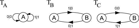
Figure 1: Example $\epsilon$-machines: $T_{A}$ has a single causal state and, according to its transition labels, is the identity function. $T_{B}$ consists of causal states $A$ and $B$ and two transitions. $T_{B}$ accepts two input strings, either $1010\ldots$ or $0101\ldots$, and flips $0$s to $1$s and vice versa as it produces an output string. Note that the function’s domain and range are the same. $T_{C}$ has the same domain and range as $T_{B}$, but does not exchange $0$s and $1$s.

Given that $\epsilon$-machines are transformations, one can ask how much processing they do—how much structure do they add to the inputs when producing an output? Due to the properties mentioned above, one can answer this question precisely. Ignoring input and output symbols, the state-to-state transition probabilities are given by an $\epsilon$-machine’s stochastic connection matrix: $\mathbf{T}\equiv\sum_{s\in\mathcal{A}}T^{(s)}$. The causal-state probability distribution $p_{\boldsymbol{{\cal S}}}$ is given by the left eigenvector of $\mathbf{T}$ associated with eigenvalue $1$ and normalized in probability. If $M$ is an $\epsilon$-machine, then the amount of information storage it has, and can add to an input process, is given by $M$’s structural complexity

$$C_{\mu}(M)\equiv-\sum_{v\in\boldsymbol{{\cal S}}}p_{\boldsymbol{{\cal S}}}(v)\log_{2}p_{\boldsymbol{{\cal S}}}(v)~{}.$$ (4)

$\epsilon$-Machine Interaction

$\epsilon$-machines interact by functional composition. Two machines $T_{A}$ and $T_{B}$ that act on each other result in a third $T_{C}=T_{B}\circ T_{A}$, where $T_{C}$ (i) has the domain of $T_{A}$ and the range of $T_{B}$ and (ii) is minimized. If $T_{A}$ and $T_{B}$ are incompatible, e.g., the domain of $T_{B}$ does not overlap with the range of $T_{A}$, the interaction produces nothing—it is considered elastic. During composition the size of the resulting $\epsilon$-machine can grow very rapidly (geometrically): $|T_{C}|\leq|T_{B}|\times|T_{A}|$.

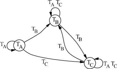
Figure 2: Interaction network for the $\epsilon$-machines of Fig. 1. It is a meta-machine.

Interaction Network

We monitor the interactions of objects in the soup via the interaction network $\mathcal{G}$. This is represented as a graph whose nodes correspond to $\epsilon$-machines and whose transitions correspond to interactions. If $T_{k}=T_{j}\circ T_{i}$ occurs in the soup, then the edge from $T_{i}$ to $T_{k}$ is labeled $T_{j}$. One can represent $\mathcal{G}$ with the binary matrices:

$$\mathcal{G}_{ij}^{(k)}=\begin{cases}1&\text{if $T_{k}=T_{j}\circ T_{i}$}\\ 0&\text{otherwise}.\end{cases}$$ (5)

For the set of $\epsilon$-machines in Fig. 1, for example, we have the interaction graph shown in Fig. 2 that is given by the matrices:

$\mathcal{G}^{(A)}=\left[\begin{matrix}1&0&0\\ 0&0&0\\ 0&0&0\end{matrix}\right]~{},$ $\mathcal{G}^{(B)}=\left[\begin{matrix}0&1&0\\ 1&0&1\\ 0&1&0\end{matrix}\right]~{},$ and $\mathcal{G}^{(C)}=\left[\begin{matrix}0&0&1\\ 0&1&0\\ 1&0&1\end{matrix}\right]~{}.$

To measure the diversity of interactions in a population we define the interaction network complexity

$$C_{\mu}({\mathcal{G}})=-\sum_{f_{i},f_{j},f_{k}>0}\frac{v_{ij}^{k}}{V^{k}}\log_{2}\frac{v_{ij}^{k}}{V^{k}}~{},$$ (6)

where

$$v_{ij}^{k}=\left\{\begin{array}[]{ll}f_{i}f_{j},&T_{k}=T_{j}\circ T_{i}\mathrm{~{}has~{}occurred,}\\ 0,&\mathrm{otherwise}~{},\end{array}\right.$$ (7)

$V^{k}=\sum_{lm}v_{lm}^{k}$ is a normalizing factor, and $f_{i}$ is the fraction of $\epsilon$-machine type $i$ in the soup. In order to emphasize our interest in actual reproduction pathways, we consider only those that have occurred in the soup.

Meta-Machines

Given a population $\mathcal{P}$ of $\epsilon$-machines, we define a meta-machine $\Omega\subset\mathcal{P}$ to be a connected set of $\epsilon$-machines that is invariant under composition. That is, $\Omega$ is a meta-machine if and only if (i) $T_{j}\circ T_{i}\in\Omega$ for all $T_{i},T_{j}\in\Omega$, (ii) for all $T_{k}\in\Omega$, there exists $T_{i},T_{j}\in\Omega$ such that $T_{k}=T_{j}\circ T_{i}$, and (iii) there is a nondirected path between every pair of nodes in $\Omega$’s interaction network $\mathcal{G}_{\Omega}$. The interactions in Fig. 2 describe a meta-machine of Fig. 1’s $\epsilon$-machines.

The meta-machine captures the notion of a self-replicating and autonomous entity and is consistent with Maturana and Varela’s autopoietic set [Varela et al., 1974], Eigen and Schuster’s hypercycle [Schuster, 1977] and Fontana and Buss’ organization [Fontana and Buss, 1996].

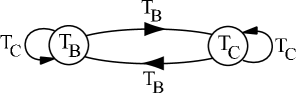
Figure 3: The meta-machine to which that in Fig. 2 decays under the population dynamics of Eq. (8).

Population Dynamics

We employ a continuously stirred flow reactor with an influx rate $\Phi_{in}$ that consists of a population $\mathcal{P}$ of $N$ $\epsilon$-machines. The dynamics of the population is iteratively ruled by compositions and replacements as follows:

1. $\epsilon$-machine Generation:

   1. With probability $\Phi_{in}$ generate a random $\epsilon$-machine $T_{R}$ (influx).

   2. With probability $1-\Phi_{in}$ (reaction):

      1. Select $T_{A}$ and $T_{B}$ randomly.

      2. Form the composition $T_{C}=T_{B}\circ T_{A}$.

2. $\epsilon$-machine Outflux:

   1. Select an $\epsilon$-machine $T_{D}$ randomly from the population.

   2. Replace $T_{D}$ with either $T_{C}$ or $T_{R}$.

Below, $T_{R}$ will be uniformly sampled from the set of all two-state $\epsilon$-machines. This set is also used when initializing the population. The insertion of $T_{R}$ corresponds to the influx while the removal of $T_{D}$ corresponds to the outflux. The latter keeps the population size constant. Note that there is no spatial dependence in this model; $\epsilon$-machines are picked uniformly from the population for each replication. The finitary process soup here is a well stirred gas of reacting objects.

When there is no influx ($\Phi_{in}$=0) and the population is closed with respect to composition, the population dynamics is described by a finite-dimensional set of equations:

$$\mathbf{f}_{t}^{(k)}=\mathbf{f}_{t-1}\cdot\mathcal{G}_{ij}^{(k)}\cdot\mathbf{f}_{t-1}^{T}Z^{-1},$$ (8)

where $\mathbf{f}_{t}^{(k)}$ is the frequency of $\epsilon$-machine type $k$ at time $t$ and $Z^{-1}$ is a normalization factor.

In addition to capturing the notion of self-replicating entities, meta-machines also describe an important type of invariant set of the population dynamics. Formally, we have

$$\Omega=\mathcal{G}\circ\Omega~{}.$$ (9)

These invariant sets can be stable or unstable under the population dynamics. Note that the meta-machine of Fig. 2 is unstable: only $T_{A}$ produces $T_{A}$s. As such, over time the population dynamics will decay to the meta-machine of Fig. 3, which describes a soup consisting only of $T_{B}$s and $T_{C}$s. This example also happens to illustrate that copying—implemented here by the identity object $T_{A}$—need not dominate the population and so does not have to be removed by hand, as done in several prior pre-biotic models. It can decay away due to the intrinsic population dynamics.

Figure 4: (a) Population-averaged $\epsilon$-machine complexity $\langle C_{\mu}(T)\rangle$ and (b) run-averaged interaction network complexity $\langle C_{\mu}(\mathcal{G})\rangle$ as a function of time $t$ and influx rate $\Phi_{in}$ for a population of $N=100$ objects. (Reprinted with permission from [Crutchfield and Görnerup, 2006].)

Simulations

A system constrained by closure forms one useful base case that allows for a straightforward analysis of the population dynamics. It does not permit, however, for the innovation of structural novelties in the soup on either the level of individual objects ($\epsilon$-machines) or on the level of their interactions. What we are interested in is the possibility of open-ended evolution of $\epsilon$-machines and their meta-machines. When enabled as an open system, both with respect to composition and influx, the soup constitutes a constructive dynamical system and the population dynamics of Eq. (8) do not strictly apply. (The open-ended population dynamics of epochal evolution is required [Crutchfield and van Nimwegen, 2000].)

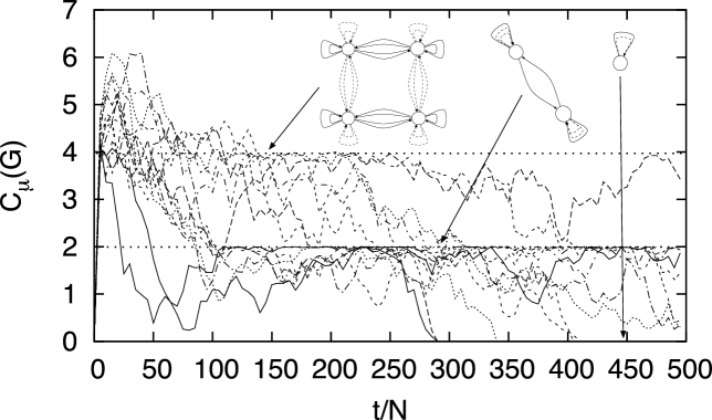
Figure 5: Meta-machine decomposition in a closed soup: 15 separate runs with $N=500$. While the minimal 4-element meta-machine $\Omega_{4}$ (shown) dominates the soup, $C_{\mu}(\mathcal{G})$ is bounded by 4 bits. Once outflux removes one of its $\epsilon$-machines, rapidly $\Omega_{4}$ decays to $\Omega_{2}$, a 2-element meta-machine (shown). ($\Omega_{4}$ does not contain a sub-meta-machine of $3$ $\epsilon$-machines.) At this point $C_{\mu}(\mathcal{G})$ is bounded by $2$ bits. After some period of time, $\Omega_{2}$ decays to $\Omega_{1}$, a single self-reproducing $\epsilon$-machine (shown), and $C_{\mu}(\mathcal{G})$ is fixed at 0.

We first set the influx rate to zero in order to study dynamics that is ruled only by compositional transformations. One important first observation is that almost the complete set of machine types that are represented in the soup’s initial random population is replaced over time. Thus, even at the earliest times, the soup generates genuine novelty. The population-averaged individual complexity $\langle C_{\mu}(T)\rangle$ increases initially, as Fig. 4(a) ($\Phi_{\mathrm{in}}\approx 0$) from [Crutchfield and Görnerup, 2006] shows. The $\epsilon$-machines are to some extent shaped by the selective pressure coming from outflux and by geometric growth due to composition. The turn-over is due to the dominance of nonreproducing $\epsilon$-machines in the initial population. $\langle C_{\mu}(T)\rangle$ subsequently declines since it is favorable to be simple as it takes a more extensive stochastic search to find reproductive interactions that include more complex $\epsilon$-machines.

Note (Fig. 4(b), $\Phi_{\mathrm{in}}\approx 0$) that the run-averaged interaction complexity $\langle C_{\mu}(\mathcal{G})\rangle$ reaches a significantly higher value than $\langle C_{\mu}(T)\rangle$, implying that the population’s structural complexity derives from its network of interactions rather than the complexity of its constituent individuals. $\langle C_{\mu}(\mathcal{G})\rangle$ continues to grow while compositional paths are discovered and created. A maximum is eventually reached after which $\langle C_{\mu}(\mathcal{G})\rangle$ declines and settles down to zero when one single type of self-reproducing $\epsilon$-machine takes over the whole population.

By monitoring the individual run values of $C_{\mu}(\mathcal{G})$ rather than the ensemble average, one sees that they form plateaus as shown in Fig. 5. The plateaus—at $C_{\mu}(\mathcal{G})=4$ bits and, most notably, at $C_{\mu}(\mathcal{G})=2$ bits and 0 bits—are determined by the largest meta-machine that is present at a given time. Being a closed set, the meta-machine does not allow any novel $\epsilon$-machines to survive and this gives the upper bound on $C_{\mu}(\mathcal{G})$. As one $\epsilon$-machine type is removed from $\Omega$ by the outflux, the meta-machine decomposes and the upper bound on $C_{\mu}(\mathcal{G})$ lowers. This produces a stepwise and irreversible succession of meta-machine decompositions.

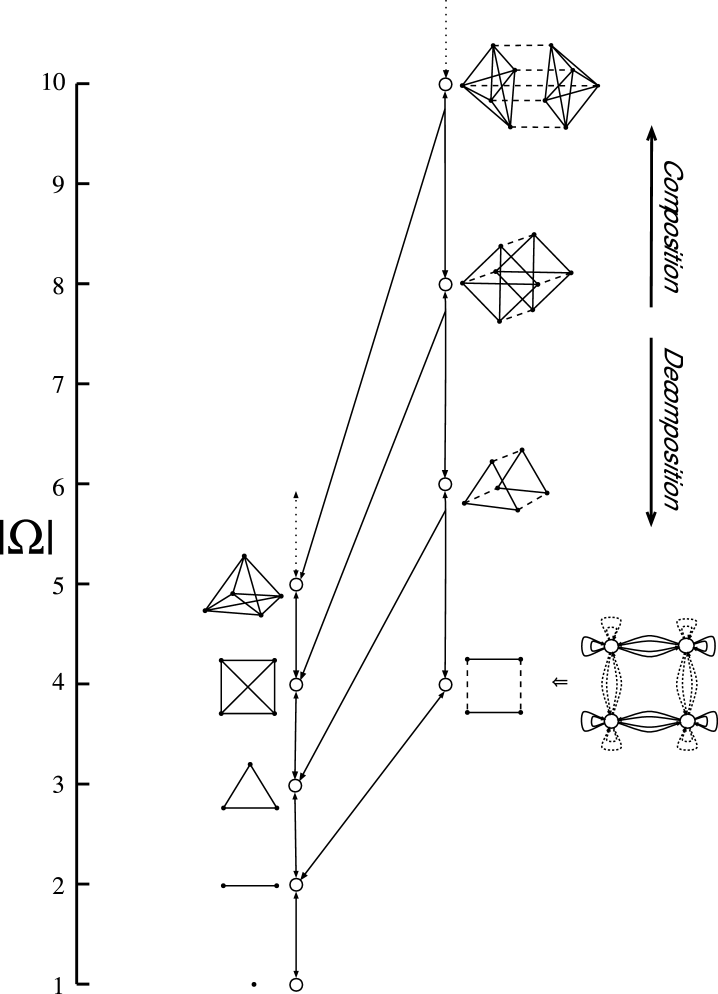
Figure 6: Meta-machine hierarchy of dynamical composition and decomposition. Dots denote $\epsilon$-machines. An isolated dot denotes a self-replicating $\epsilon$-machine. Solid lines denote $T_{A}\stackrel{{\scriptstyle T_{B}}}{{\longrightarrow}}T_{C}$ transitions. Dashed lines denote $T_{B}\stackrel{{\scriptstyle T_{A}}}{{\longrightarrow}}T_{C}$ transitions. Although all possible transitions are used by the meta-machines shown, they are represented in a simplified way according to $\Omega_{4}$; cf. Fig. 5.

Thus, in the case of zero influx, one sees that the soup moves from one extreme to another. It is completely disordered initially, generates structural complexity in its individuals and in its interaction network, runs out of resources (poorly reproducing $\epsilon$-machines that are consumed by outflux), and decomposes down to a single type of simple self-reproducing $\epsilon$-machine.

Although Fig. 5 shows only three plateaus, there is in principle one plateau for every meta-machine that at some point is the largest one generated by the soup. The diagram in Fig. 6 summarizes our results from a more extensive and systematic survey of meta-machine hierarchies from a series of runs with $N=500$. It gives one illuminating example of how the soup spontaneously generates hierarchies of meta-machines.

Leaving closed soups behind, we now investigate the effects of influx. Recall the population-averaged $\epsilon$-machine complexity $\langle C_{\mu}(T)\rangle$ and the run-averaged interaction network complexity $\langle C_{\mu}(\mathcal{G})\rangle$ as a function of $t$ and $\Phi_{in}$ shown in Fig. 4. Over time, $\langle C_{\mu}(T)\rangle$ behaves similarly for $\Phi_{in}>0$ as it does when $\Phi_{in}=0$. It increases rapidly initially, reaches a peak, and declines to a steady state. Notably, the emergence of complex organizations of interaction networks occurs where the average structural complexity of the $\epsilon$-machines is low. Stationary $\langle C_{\mu}(T)\rangle$ is instead maximized at a relatively high influx rate ($\Phi_{in}\approx 0.75$) at which $\langle C_{\mu}(\mathcal{G})\rangle$ is small compared to its maximum. As $\Phi_{in}$ is increased, so is $\langle C_{\mu}(\mathcal{G})\rangle$ at large times. $\langle C_{\mu}(\mathcal{G})\rangle$ is maximized around $\Phi_{in}\approx 0.1$. For higher influx rates, individual novelty has a deleterious effect on the sophistication of a population’s interaction network. Existing reproductive paths do not persist due to the low rate of successful compositions of highly structured (and so specialized) individuals. We found that the maximum network complexity $\widehat{C_{\mu}}(\mathcal{G})$ grows slowly and linearly over time at $\approx 7.6\cdot 10^{-4}$ bits/replication.

Summary and Conclusions

To understand the basic mechanisms driving the evolutionary emergence of structural complexity in a quantitative and tractable pre-biotic setting, we investigated a well stirred soup of $\epsilon$-machines (finite-memory communication channels) that react with each other by composition and so generate new $\epsilon$-machines. When the soup is open with respect to composition and influx, it spontaneously builds structural complexity on the level of transformative relations among the $\epsilon$-machines rather than in the $\epsilon$-machine individuals themselves. This growth is facilitated by the use of relatively non-complex individuals that represent general and elementary local functions rather than highly specialized individuals. The soup thus maintains local simplicity and generality in order to build up hierarchical structures that support global complexity. Novel computational representations are intrinsically introduced in the form of meta-machines that, in turn, are interrelated in a hierarchy of composition and decomposition. Computationally powerful local representations are thus not necessary (nor effective) in order for the emergence and growth of complex replicative processes in the finitary process soup. Meta-machines in closed soups eventually decay. For $C_{\mu}(\mathcal{G})$ to maintain and grow the soup must be fed with novel material in the form of random $\epsilon$-machines. Otherwise, any spontaneously generated meta-machines are decomposed (due to finite-population sampling) and the population eventually consists of a single type of trivially self-reproducing $\epsilon$-machine. At an intermediate influx rate, however, the interaction network complexity is not only maintained but grows linearly with time. This, then, suggests the possibility of open-ended evolution of increasingly sophisticated organizations.

References

- Adami and Brown, 1994 Adami, C. and Brown, C. T. (1994). Evolutionary learning in the 2d artificial life system ‘Avida’. In Artificial Life 4, pages 377–381. MIT Press.
- Bagley et al., 1989 Bagley, R. J., Farmer, J. D., Kauffman, S. A., Packard, N. H., Perelson, A. S., and Stadnyk, I. M. (1989). Modeling adaptive biological systems. Biosystems, 23:113–138.
- Brookshear, 1989 Brookshear, J. G. (1989). Theory of computation: Formal languages, automata, and complexity. Benjamin/Cummings, Redwood City, California.
- Cover and Thomas, 1991 Cover, T. M. and Thomas, J. A. (1991). Elements of Information Theory. Wiley-Interscience, New York.
- Crutchfield, 1994 Crutchfield, J. P. (1994). The calculi of emergence: Computation, dynamics, and induction. Physica D, 75:11 – 54.
- Crutchfield and Görnerup, 2006 Crutchfield, J. P. and Görnerup, O. (2006). Objects that make objects: The population dynamics of structural complexity. J. Roy. Soc. Interface, in press.
- Crutchfield and Mitchell, 1995 Crutchfield, J. P. and Mitchell, M. (1995). The evolution of emergent computation. Proc. Natl. Acad. Sci., 92:10742–10746.
- Crutchfield and van Nimwegen, 2000 Crutchfield, J. P. and van Nimwegen, E. (2000). The evolutionary unfolding of complexity. In Landweber, L. F. and Winfree, E., editors, Evolution as Computation, Natural Computing Series, page to appear, New York. Springer-Verlag. Santa Fe Institute Working Paper 99-02-015; adap-org/9903001.
- Crutchfield and Young, 1989 Crutchfield, J. P. and Young, K. (1989). Inferring statistical complexity. Phys. Rev. Let., 63:105–108.
- Farmer et al., 1986 Farmer, J. D., Packard, N. H., and Perelson, A. S. (1986). The immune system, adaptation, and machine learning. Phys. D, 2(1-3):187–204.
- Fontana, 1991 Fontana, W. (1991). Algorithmic chemistry. In Langton, C., Taylor, C., Farmer, J. D., and Rasmussen, S., editors, Artificial Life II, volume XI of Santa Fe Institute Stuides in the Sciences of Complexity, pages 159–209, Redwood City, California. Addison-Wesley.
- Fontana and Buss, 1996 Fontana, W. and Buss, L. W. (1996). The barrier of objects: From dynamical systems to bounded organizations’. In Casti, S. and Karlqvist, A., editors, Boundaries and Barriers, pages 56–116. Addison-Wesley.
- Hopcroft and Ullman, 1979 Hopcroft, J. E. and Ullman, J. D. (1979). Introduction to Automata Theory, Languages, and Computation. Addison-Wesley, Reading.
- Lynch and Conery, 2003 Lynch, M. and Conery, J. S. (2003). The origins of genome complexity. Science, 302:1401–1404.
- Rasmussen et al., 1990 Rasmussen, S., Knudsen, C., Feldberg, P., and Hindsholm, M. (1990). The coreworld: Emergence and evolution of cooperative structures in a computational chemistry. In Emergent Computation, pages 111–134. North-Holland Publishing Co.
- Rasmussen et al., 1992 Rasmussen, S., Knudsen, C., and Feldberg, R. (1992). Dynamics of programmable matter. In Artificial Life II: Proceedings of an Interdisciplinary Workshop on the Synthesis and Simulation of Living Systems (Santa Fe Institute Studies in the Sciences of Complexity, Vol. 10). Addison-Wesley.
- Rat Genome Sequencing Project Consortium, 2004 Rat Genome Sequencing Project Consortium (2004). Genome sequence of the brown norway rat yields insights into mammalian evolution. Nature, 428:493–521.
- Ray, 1991 Ray, T. S. (1991). An approach to the synthesis of life. In Langton, C., Taylor, C., Farmer, J. D., and Rasmussen, S., editors, Artificial Life II, volume XI of Santa Fe Institute Stuides in the Sciences of Complexity, pages 371–408, Redwood City, California. Addison-Wesley.
- Rössler, 1979 Rössler, O. (1979). Recursive evolution. BioSystems, 11:193–199.
- Schrödinger, 1967 Schrödinger, E. (1967). What is Life? Mind and Matter. Cambridge Univ. Press, Cambridge, United Kingdom.
- Schuster, 1977 Schuster, P. (1977). The hypercycle: A principle of natural self-organization. Naturwissenschaften, 64:541–565.
- Varela et al., 1974 Varela, F. J., Maturana, H. R., and Uribe, R. (1974). Autopoiesis: The organization of living systems. BioSystems, 5(4):187–196.
- von Neumann, 1966 von Neumann, J. (1966). Theory of Self-Reproducing Automata. University of Illinois Press, Urbana.