Multiresolution analysis of fluctuations in non-stationary time series through discrete wavelets

Abstract

We illustrate the efficacy of a discrete wavelet based approach to characterize fluctuations in non-stationary time series. The present approach complements the multi-fractal detrended fluctuation analysis (MF-DFA) method and is quite accurate for small size data sets. As compared to polynomial fits in the MF-DFA, a single Daubechies wavelet is used here for de-trending purposes. The natural, built-in variable window size in wavelet transforms makes this procedure well suited for non-stationary data. We illustrate the working of this method through the analysis of binomial multi-fractal model. For this model, our results compare well with those calculated analytically and obtained numerically through MF-DFA. To show the efficacy of this approach for finite data sets, we also do the above comparison for Gaussian white noise time series of different size. In addition, we analyze time series of three experimental data sets of tokamak plasma and also spin density fluctuations in 2D Ising model.

I Introduction

For non-stationary time series, it is of vital importance to ’correctly’ separate fluctuations from average behavior (trend), for studying various properties of real systems having complex dynamics – i.e., having many different spatio-temporal scales. Several techniques have been developed to carry out this separation. Among these are, de-trended fluctuation analysis and its variants peng ; net and the wavelet transform daub ; mall based multi-resolution analysis mani ; ran . These methods and earlier methods mandel ; arn1 have found wide application in analysis of correlations and characterization of scaling behavior of time-series data in, physiology, finance, and natural sciences khu ; gopi ; ple ; chen ; matia ; krs ; phand ; xu ; nico ; gu ; sade . Recently, the relative merits of MF-DFA and a variety of other approaches to characterize fluctuations have been carried out jaro . It is worth emphasizing that fluctuation analysis and characterization have been earlier attempted using Haar wavelets, in the context of bio-medical applications, without the study of scaling behavior pkp1 ; pkp2 .

In this paper, we present a refined version of our earlier procedure mani , where a local averaging procedure is adopted to accurately separate fluctuations, from the trend, akin to the MF-DFA approach. It is important to further emphasize that, in our earlier method, global averaging had been carried out for finding the fluctuations. This necessitated the use of two wavelet basis to separate large and small fluctuations. In comparison, here we find that a single Daubechies wavelet enables one to study small and large fluctuations together. The effect of correlation of non-stationary data on the fluctuations are clearly isolated.

Details of the present approach are described in Sec. II. Sec. III contains analysis of fluctuations of the binomial multi-fractal model and comparison of results using different approaches. To check the efficacy of the present method, when the data size is small, we have carried out a systematic investigation of the scaling exponents for the Gaussian white noise of different sizes using a number of wavelets belonging to Daubechies family, which is then compared with MF-DFA with polynomial fits of different degrees. It is found that for a small length data the present wavelet based method is better suited to estimate the scaling exponents. The results illustrate the correctness of our approach, aside from being theoretically sound and natural. Subsequently, we carry out analysis of fluctuation data observed in tokamak plasma depicted in Fig. 1. Results describing scaling properties of tokamak plasma are given in Sec. IV. We also analyze the fluctuation characteristics of the spin density of the 2D Ising model. Finally, in Sec. V we summarize our findings and give some concluding remarks.

II Details of modified wavelet approach

The present wavelet based procedure is explained through the following steps. Note that the steps are very similar to those in MF-DFA net , except that in order to detrend, we use wavelets and MF-DFA uses local polynomial fits.

Let $x_{t}$ (t=1,2,3,…,N) be the time series of length N. First determine the ”profile” (say $Y(i)$), which is cumulative sum of series after subtracting the mean.

$$Y(i)=\sum_{t=1}^{i}[x_{t}-\langle x\rangle],~{}~{}~{}i=1,....,N.$$ (1)

Next, we carry out wavelet transform on the profile $Y(i)$ to separate the fluctuations from the trend. For this purpose, discrete wavelets belonging to Daubechies (Db) family is used. It is worth repeating that these wavelets satisfy the vanishing moment conditions: $\int t^{m}\psi_{j,k}(t)dt=0$, where $0\leq m<n$. Because of this, the low-pass coefficients keep track of the polynomial trends in the data. For example, the low-pass coefficients in Db-4, Db-6 and Db-8, retain polynomial trend which are linear, quadratic and cubic respectively. Hence, reconstruction using these low-pass coefficients alone is quite accurate in extracting the local trend, in a desired window size. The fluctuations are then extracted at each level by subtracting the obtained time series from the original data. Though the Daubechies wavelets extract the fluctuations nicely, its asymmetric nature and wrap around problem affects the precision of the values. This is corrected by applying wavelet transform to the reverse profile, to extract a new set of fluctuations. These fluctuations are then reversed and averaged over the earlier obtained fluctuations. These are the fluctuations (at a particular level), which we consider for analysis.

The extracted fluctuations are subdivided into non-overlapping segments $M_{s}=int(N/s)$ where $s=2^{(L-1)}W$ is the wavelet window size at a particular level (L) for the chosen wavelet. Here $W$ is the number of filter coefficients of the discrete wavelet transform basis under consideration. For example, with Db-4 wavelet with 4 filter coefficients, $s=4$ at level 1 and $s=8$ at level 2 and so on. It is obvious that some data points would have to be discarded, in case $N/s$ is not an integer. This causes statistical errors in calculating the local variance. In such cases, we have to repeat the above procedure starting from the end and going to the beginning to calculate the local variance.

The $q^{th}$ order fluctuation function, $F_{q}(s)$ is obtained by squaring and averaging fluctuations over all segments:

$$F_{q}(s)\equiv\{\frac{1}{2M_{s}}\sum_{b=1}^{2M_{s}}[F^{2}(b,s)]^{q/2}\}^{1/q}.$$ (2)

Here ’q’ is the order of moment that can take any real value. The above procedure is repeated for variable window sizes for different value of q (except q=0). The scaling behavior is obtained by analyzing the fluctuation function,

$$F_{q}(s)\sim s^{h(q)},$$ (3)

in a logarithmic scale for each value of q. If the order $q=0$, direct evaluation of Eq. (2) leads to divergence of the scaling exponent. In that case, logarithmic averaging has to be employed to find the fluctuation function;

$$F_{q}(s)\equiv exp\{\frac{1}{2M_{s}}\sum_{b=1}^{2M_{s}}ln[F^{2}(b,s)]^{q/2}\}^{1/q}.$$ (4)

As is well-known, if the time series is mono-fractal, the h(q) values are independent of q. For multifractal time series, h(q) values depend on q. The correlation behavior is characterized from the Hurst exponent ($H=h(q=2)$), which varies from $0<H<1$. For long range correlation, $H>0.5$, $H=0.5$ for uncorrelated and $H<0.5$ for long range anti-correlated time series.

The behavior of fluctuations extracted through multifractal detrended fluctuation analysis and fluctuations obtained using wavelet transform are shown in Fig. 2 and Fig.3 respectively. We note that the fluctuations extracted from the two methods differ at the boundaries.

III Analysis of Binomial multifractal model

For the multifractal time series generated through the binomial multifractal model feder ; barba ; pei , a series of $N=2^{n_{max}}$ numbers $x_{j}$, with $j=1,...,N$, is defined by

$$x_{j}=a^{n(j-1)}(1-a)^{n_{max}-n(j-1)},$$ (5)

where $0.5<a<1$ is a parameter and $n(j)$ is the number of digits equal to $0$ or $1$ in the binary representation of the index $j$. The scaling exponent $h(q)=\frac{1}{q}-\frac{ln[a^{q}+(1-a)^{q}]}{qln(2)}$ and $\tau(q)=\frac{-ln[a^{q}+(1-a)^{q}]}{ln(2)}$ can be calculated exactly in this model. These would be compared with numerical results obtained through wavelet analysis, for illustrating the efficacy of our procedure.

In our wavelet based analysis, profile of the binomial multifractal model time series has been subjected to a multi-level wavelet decomposition. The length of the data should be $2^{N}$, otherwise constant padding is added at the ends.

In Table-1, we give the $h(q)$ values for various $q$, obtained from analytical results, MF-DFA and wavelet (Db-8) based method for binomial multifractal series. In MF-DFA, we have used a quadratic polynomial fit for extracting fluctuations. It is clear from the given tables, that the wavelet estimate of the $h(q)$ exponent for the binomial multifractal time series, is extremely reliable.

q	$h(q)_{BMFS_{a}}$	$h(q)_{BMFS_{s}}$	$h(q)_{BMFS_{w}}$
-10	1.9000	1.9304	1.8991
-9	1.8889	1.9184	1.8879
-8	1.8750	1.9032	1.8740
-7	1.8572	1.8837	1.8560
-6	1.8337	1.8576	1.8319
-5	1.8012	1.8210	1.7981
-4	1.7544	1.7663	1.7473
-3	1.6842	1.6783	1.6641
-2	1.5760	1.5397	1.5218
-1	1.4150	1.3939	1.3828
0	0	1.2030	1.2163
1	1.0000	0.9934	1.0091
2	0.8390	0.8312	0.8453
3	0.7309	0.7234	0.7359
4	0.6606	0.6538	0.6649
5	0.6139	0.6075	0.6177
6	0.5814	0.5753	0.5848
7	0.5578	0.5519	0.5610
8	0.5400	0.5343	0.5430
9	0.5261	0.5205	0.5290
10	0.5150	0.5095	0.5178

Table 1: The $h(q)$ values of binomial multi-fractal series (BMFS) computed analytically ($BMFS_{a}$), through MF-DFA ($BMFS_{s}$) and wavelet ($BMFS_{w}$) approach, Db-8 wavelet has been used.

In our earlier method, we had used two different wavelets for analyzing the large and small fluctuations. We see that, for the computer generated BMF model time series, the present method, with only a single wavelet, is quite efficient for characterizing the correlation properties and multifractal behavior of non-stationary time series. Our results compare very well with the analytical results and MF-DFA calculation. It is worth pointing out that, we have carried out analysis using Daubechies wavelets of various order. It was found that Db-8 performs the best. The improvement with higher wavelet is minimal.

For the purpose of finding out the efficacy of the present method when the data size is small, we now study the Gaussian white noise of lengths 1000, 5000, 10000 and 50000 points. These are analyzed through Daubechies 4 (Db-4) to Daubechies 8 wavelets. For the purpose of MF-DFA, we have computed the trend using linear, quadratic and cubic polynomial fits. The results are depicted in Table II, III, IV and V. It is observed that for smaller size data, wavelet based method is quite effective in estimating the scaling exponent. In this approach, one wavelet basis is found to be effective in capturing both smaller and larger fluctuations as compared to the earlier approach. The local procedure adopted here is responsible for this improvement.

IV Analysis of Experimental and synthetic data sets

We have analyzed three sets of experimentally observed time series of variables in ohmically heated edge plasma in Aditya tokamak jos . The time series are i) ion saturation current, ii) ion saturation current when the probe is in the limiter shadow, and iii) floating potential, 6mm inside the main plasma. Each time series has about 24,000 data points sampled at 1MHZ jha . These are shown in Fig. 1. The study of fluctuations play an important role in our understanding of turbulent transport of particles and heat in the plasma.

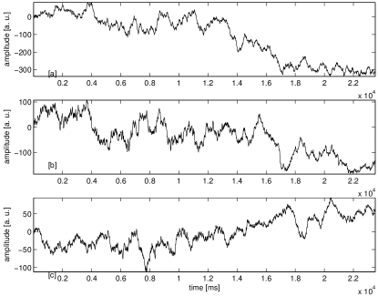
Figure 1: Time series of (a) ion saturation current, (b) floating potential, 6mm inside the main plasma and (c) ion saturation current, when the probe is in the limiter shadow. Each time series is of approx. 24,000 data points.

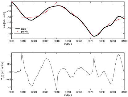
Figure 2: Fluctuations extracted from the time series of ion saturation current, when the probe is in the limiter shadow using MF-DFA (window size is 32).

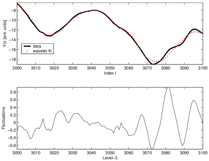
Figure 3: Fluctuations extracted from the time series of ion saturation current, when the probe is in the limiter shadow, at level-3 using Db-8 wavelet (window size 32).

Fluctuation function $F_{q}(s)$ for various values of q, for the time series of three experimental data sets are computed using Db-8 wavelet. In Fig. 4, we have shown $F_{q}(s)$ versus $s$ of the time series of ion saturation current, when the probe is in the limiter shadow.

We have calculated scaling exponents $h(q)$ and $\tau(q)=qh(q)$ for various $q$ values. All the three time series exhibit non-linear (fractal) behavior for $h(q)$ values, as a function of $q$. From the measured Hurst exponent, it was found that the three time series possess long range correlations, whereas for the shuffled time series, the same is absent. However the shuffled time series still shows multifractality, which is clearly seen in Table-VI. Here, the $h(q)$ values of time series and shuffled time series of i) ion saturation current (IS), ii) ion saturation current, when the probe is in the limiter shadow (ISC) and iii) floating potential, 6mm inside the main plasma (FP) are given, with the subscript ’s’ referring to shuffled time series.

The multifractal behavior of the experimental data set can also be studied from the $f(\alpha)$ spectrum. The $f(\alpha)$ values are obtained from the Legendre transform of $\tau(q)$. Explicitly, $f(\alpha)\equiv q\alpha-\tau(q)$, where $\alpha\equiv\frac{d\tau(q)}{dq}$. For monofractal time series, $\alpha=const.$, whereas for multifractal time series there will be a distribution of $\alpha$ values. Fig. 5 shows the $f(\alpha)$ spectrum. In the unshuffled data, one observes a broader spectrum, whereas for the shuffled data, where the correlation is lost, the same is narrower.

We now proceed to study the scaling behavior of the spin densities below and at critical temperature for the 2D Ising model, which are shown in Fig.6, as a function of time. The spin densities are computed following the procedure described earlier in Ref.mani ; hwa . Below the critical temperature, the fluctuations show Gaussian white noise character. At critical temperature the spin densities show a multifractal behavior with long range correlations, as expected from physical ground. Both these aspects are clearly shown in Fig. 7.

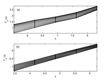
Figure 4: The log-log plot of fluctuation function $F_{q}(s)$ vs $s$ for various values of $q$ (a) for the time series of ion saturation current, when the probe is in the limiter shadow and (b) for its shuffled time series, using Db-8 wavelet.

Figure 5: The multi-fractal behavior of different type of experimental data sets is shown through the $f(\alpha)$ spectra for unshuffled and shuffled time series. Here the subscript ’s’ in IC, ISC and FP refers to the shuffled time series. One observes a broader spectra for the correlated, unshuffled case.

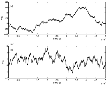
Figure 6: The integrated time series of average spin densities after subtraction of the mean, [a] at $T=1.0$, below $T_{c}$ and [b] $T_{c}=2.27$. The difference in behavior of the fluctuations at different temperatures is clearly visible.

Figure 7: For time series [a] Below $T_{c}$, $h(q)$ shows linear behavior for different values $q$, indicating a monofractal behavior and [b] the non-linear behavior of $h(q)$ for different values of $q$ at $T_{c}$, shows clearly the long-range correlation and multifractal nature.

q	Db4	Db6	Db8	Linear	Quadratic	Cubic
-10	0.59008	0.58762	0.6018	0.67735	0.5487	0.57551
-9	0.58467	0.58343	0.59477	0.6665	0.54552	0.57085
-8	0.57877	0.57889	0.5876	0.65406	0.54215	0.56572
-7	0.57246	0.57401	0.5805	0.63991	0.5386	0.56003
-6	0.56591	0.5689	0.57376	0.62404	0.53487	0.55371
-5	0.55936	0.56368	0.56763	0.6066	0.53096	0.5467
-4	0.55318	0.55855	0.56228	0.58806	0.52689	0.53896
-3	0.5477	0.5537	0.5578	0.56905	0.52271	0.53052
-2	0.54321	0.54924	0.55419	0.55027	0.51847	0.5215
-1	0.53981	0.54508	0.55133	0.53218	0.51426	0.51214
0	0.53738	0.54099	0.54901	0.51487	0.51017	0.50279
1	0.53554	0.53672	0.54693	0.49815	0.50623	0.49384
2	0.53374	0.53211	0.54473	0.48183	0.5024	0.48562
3	0.53148	0.52714	0.54204	0.46604	0.49851	0.47834
4	0.52845	0.52187	0.53859	0.45121	0.49433	0.47201
5	0.52458	0.5164	0.53424	0.43786	0.48969	0.46655
6	0.51997	0.51082	0.52903	0.42632	0.48453	0.46176
7	0.5148	0.50527	0.52313	0.41665	0.47894	0.4575
8	0.50928	0.49982	0.5168	0.40869	0.47309	0.45362
9	0.50365	0.49458	0.51035	0.40218	0.46718	0.45002
10	0.49808	0.4896	0.50401	0.39684	0.46138	0.44664

Table 2: The $h(q)$ values of Gaussian white noise (of data length $1000$) calculated through wavelets from Daubechies family and MF-DFA.

q	Db4	Db6	Db8	Linear	Quadratic	Cubic
-10	0.55498	0.52839	0.54909	0.5331	0.5637	0.59861
-9	0.55122	0.5249	0.54704	0.53022	0.55758	0.58947
-8	0.54716	0.52141	0.54494	0.5276	0.55133	0.57984
-7	0.54282	0.51797	0.5428	0.52539	0.54511	0.56988
-6	0.53822	0.51464	0.5406	0.52371	0.53909	0.55977
-5	0.53343	0.51141	0.53832	0.52267	0.53343	0.54968
-4	0.52853	0.50829	0.53594	0.52225	0.52825	0.53979
-3	0.5236	0.50524	0.53345	0.52226	0.52361	0.5302
-2	0.51874	0.50221	0.53083	0.52231	0.5195	0.521
-1	0.514	0.49913	0.52808	0.52183	0.51581	0.51223
0	0.50944	0.49593	0.52518	0.52025	0.5124	0.50387
1	0.50506	0.49253	0.52214	0.51722	0.50907	0.49595
2	0.50083	0.48886	0.51896	0.51271	0.5056	0.48845
3	0.49668	0.48485	0.51566	0.50707	0.50174	0.48141
4	0.49253	0.48045	0.51225	0.50076	0.49728	0.47482
5	0.4883	0.47565	0.50875	0.49425	0.49208	0.46866
6	0.48398	0.47046	0.5052	0.48785	0.48611	0.46286
7	0.47957	0.46495	0.50162	0.48172	0.47948	0.45739
8	0.47512	0.45923	0.49805	0.47593	0.47243	0.45221
9	0.47072	0.45345	0.49453	0.4705	0.46525	0.44732
10	0.46643	0.44776	0.49109	0.46543	0.45818	0.44274

Table 3: The $h(q)$ values of Gaussian white noise (of data length $5000$) calculated through Daubechies 4 (Db-4) to Daubechies 8 wavelets and MF-DFA.

q	Db4	Db6	Db8	Linear	Quadratic	Cubic
-10	0.62408	0.56361	0.56012	0.55754	0.58706	0.58575
-9	0.61137	0.55897	0.55515	0.55431	0.57652	0.58211
-8	0.59803	0.55425	0.55031	0.5511	0.56615	0.5787
-7	0.58486	0.54953	0.54562	0.54805	0.55607	0.57562
-6	0.57282	0.54489	0.54108	0.5454	0.54631	0.57298
-5	0.56253	0.54043	0.53669	0.54342	0.53685	0.57083
-4	0.55405	0.53623	0.53244	0.5425	0.52759	0.56919
-3	0.54705	0.53236	0.52831	0.54308	0.51845	0.56802
-2	0.54104	0.52891	0.52427	0.54554	0.50934	0.5672
-1	0.53565	0.5259	0.52031	0.55009	0.50025	0.56657
0	0.53055	0.52336	0.51644	0.55644	0.49128	0.5659
1	0.52554	0.52128	0.51263	0.56367	0.48267	0.56495
2	0.52043	0.51963	0.5089	0.57032	0.47483	0.56351
3	0.51507	0.51835	0.50525	0.57505	0.46834	0.56138
4	0.50933	0.51737	0.5017	0.57717	0.46375	0.55845
5	0.50314	0.51662	0.49824	0.57678	0.46144	0.55471
6	0.49648	0.516	0.49488	0.57446	0.46132	0.55023
7	0.48944	0.51543	0.49164	0.57092	0.46277	0.54513
8	0.48217	0.51482	0.48851	0.56675	0.46493	0.53964
9	0.47485	0.51412	0.48552	0.56236	0.46699	0.53395
10	0.46768	0.51331	0.48267	0.55802	0.46847	0.52826

Table 4: The $h(q)$ values of Gaussian white noise (of data length $10000$) calculated through Daubechies 4 (Db-4) to Daubechies 8 wavelets and MF-DFA.

q	Db4	Db6	Db8	Linear	Quadratic	Cubic
-10	0.50973	0.50575	0.50463	0.59746	0.51373	0.49263
-9	0.50728	0.50268	0.50228	0.58828	0.50577	0.49219
-8	0.505	0.4998	0.50021	0.57966	0.49807	0.49214
-7	0.5029	0.49718	0.49839	0.57196	0.49083	0.49261
-6	0.50099	0.49486	0.4968	0.56548	0.48421	0.49371
-5	0.49922	0.49291	0.49544	0.56046	0.47833	0.49556
-4	0.49756	0.49138	0.49427	0.55703	0.47332	0.49827
-3	0.49599	0.49032	0.4933	0.55517	0.46924	0.50194
-2	0.49451	0.48979	0.49251	0.55478	0.46613	0.50674
-1	0.49315	0.48983	0.49191	0.55561	0.46399	0.51299
0	0.49196	0.49047	0.49149	0.55732	0.46278	0.52127
1	0.49098	0.49167	0.49126	0.55941	0.4624	0.53257
2	0.49027	0.49335	0.49119	0.56124	0.46269	0.54818
3	0.48983	0.49536	0.49126	0.56217	0.46346	0.56935
4	0.48967	0.4975	0.49142	0.56172	0.46451	0.59634
5	0.48975	0.49955	0.4916	0.55975	0.46563	0.6275
6	0.48998	0.50133	0.49172	0.55647	0.46665	0.65973
7	0.49028	0.50269	0.4917	0.55225	0.46748	0.68996
8	0.49057	0.50356	0.49147	0.54745	0.46805	0.71637
9	0.49077	0.50396	0.49099	0.5424	0.46836	0.73842
10	0.49085	0.50391	0.49024	0.53731	0.46842	0.75633

Table 5: The $h(q)$ values of Gaussian white noise (of data length $50000$) calculated through Daubechies 4 (Db-4) to Daubechies 8 wavelets and MF-DFA.

q	$h(q)_{IC}$	$h(q)_{IC_{s}}$	$h(q)_{ISC}$	$h(q)_{ISC_{s}}$	$h(q)_{FP}$	$h(q)_{FP_{s}}$
-10	0.7233	0.5325	0.7308	0.5416	0.6684	0.5309
-9	0.7178	0.5284	0.7243	0.5383	0.6669	0.5282
-8	0.7119	0.5244	0.7173	0.5350	0.6655	0.5254
-7	0.7055	0.5205	0.7097	0.5317	0.6643	0.5224
-6	0.6987	0.5169	0.7017	0.5285	0.6632	0.5193
-5	0.6916	0.5134	0.6936	0.5254	0.6616	0.5162
-4	0.6844	0.5102	0.6857	0.5224	0.6585	0.5130
-3	0.6771	0.5072	0.6781	0.5194	0.6526	0.5097
-2	0.6698	0.5044	0.6710	0.5166	0.6424	0.5065
-1	0.6625	0.5018	0.6644	0.5138	0.6279	0.5034
0	0.6553	0.4994	0.6580	0.5109	0.6105	0.5003
1	0.6482	0.4972	0.6518	0.5081	0.5921	0.4973
2	0.6410	0.4951	0.6458	0.5052	0.5743	0.4943
3	0.6337	0.4932	0.6401	0.5024	0.5579	0.4915
4	0.6262	0.4915	0.6347	0.4995	0.5435	0.4887
5	0.6186	0.4898	0.6297	0.4967	0.5311	0.4860
6	0.6110	0.4883	0.6251	0.4939	0.5205	0.4833
7	0.6035	0.4869	0.6209	0.4911	0.5116	0.4805
8	0.5963	0.4855	0.6171	0.4884	0.5043	0.4778
9	0.5896	0.4842	0.6137	0.4857	0.4981	0.4750
10	0.5833	0.4829	0.610	0.4831	0.4929	0.4723

Table 6: The $h(q)$ values of time series and shuffled time series of i) ion saturation current (IS), ii) ion saturation current, when the probe is in the limiter shadow (ISC) and iii) floating potential, 6mm inside the main plasma (FP). Here the subscript ’s’ refers values of shuffled time series. The Hurst measure is closer to Brownian motion (H=0.5) for the shuffled times series, where as for the unshuffled case, the presence of long range correlation brings in substantial deviations.

V Conclusion

In conclusion, we have presented a reliable discrete wavelet based method for estimating correlation and multiscaling behavior. This approach is quite efficient and accurate in characterizing the behavior of diverse non-stationary time series. Its efficacy is derived from the optimal window size of discrete wavelet basis. A single wavelet from Daubechies family is found to be good for analyzing both the small and large fluctuations. The averaging over the fluctuations from forward and backward procedure took good care of both small and large fluctuations.

Acknowledgements We would like to thank Dr. R. Jha for providing the tokamak plasma data for analysis and Ms. Namrata Shah for helping us in preparing this manuscript.

References

- (1) C. K. Peng, S. V. Buldyrev, S. Havlin, M. Simons, H. E. Stanley, and A. L. Goldberger, Phys. Rev. E 49, 1685 (1994).
- (2) J. W. Kantelhardt, D. Rybskia, S. A. Zschiegnerb, P. Braunc, E. Koscielny-Bundea, V. Livinae, S. Havline, A. Bundea, and H. E. Stanley, Physica A 330, 240 (2003).
- (3) I. Daubechies, Ten lectures on wavelets (SIAM, Philadelphia, 1992).
- (4) S. Mallat, A Wavelet Tour of Signal Processing (Academic Press, 1999).
- (5) P. Manimaran, P.K. Panigrahi, and J.C. Parikh, Phys. Rev. E 72, 046120 (2005).
- (6) P. Manimaran, P. A. Lakshmi and P. K. Panigrahi, J. Phys. A: Math. Gen. 39, L599 (2006).
- (7) B. B. Mandelbrot, and J. W. van Ness, SIAM Review 10, 422 (1968); B. B. Mandelbrot, Fractals and Scaling in Finance: Discontinuity, Concentration, Risk (Springer Verlag, New York, 1997).
- (8) A. Arneodo, G. Grasseau, and M. Holschneider, Phys. Rev. Lett. 61, 2281 (1988); J. F. Muzy, E. Bacry, and A. Arneodo, Phys. Rev. E 47, 875 (1993).
- (9) K. Hu, P. Ch. Ivanov, Z. Chen, P. Carpena, and H. E. Stanley, Phys.Rev. E 64, 11114 (2001).
- (10) P. Gopikrishnan, V. Plerou, L. A. Nunes Amaral, M. Meyer, and H. E. Stanley, Phys. Rev. E 60, 5305 (1999).
- (11) V. Plerou, P. Gopikrishnan, L. A. Nunes Amaral, M. Meyer, and H. E. Stanley, Phys. Rev. E 60, 6519 (1999).
- (12) Z. Chen, P. Ch. Ivanov, K. Hu, and H. E. Stanley, Phys. Rev. E 65, 041107 (2002).
- (13) K. Matia, Y. Ashkenazy, and H. E. Stanley, Europhys. Lett. 61, 422 (2003).
- (14) R. C. Hwa, C. B. Yang, S. Bershadskii, J.J. Niemela, and K. R. Sreenivasan, Phys. Rev. E 72, 066308 (2005).
- (15) K. Ohashi, L. A. Nunes Amaral, B. H. Natelson, and Y. Yamamoto, Phys. Rev. E. 68, 065204(R) (2003).
- (16) L. Xu, P. Ch. Ivanov, K. Hu, Z. Chen, A. Carbone, and H. E. Stanley, eprint: cond-mat/0408047.
- (17) N. Brodu, eprint: nlin.CD/0511041 (2005).
- (18) G. F. Gu, and W. X. Zhou, Phys. Rev. E 74, 061104 (2006).
- (19) M. S. Movahed, and E. Hermanis, Physica A 387, 915 (2008).
- (20) P. Owiecimka, J. Kwapie and S. Drozdz, Phys. Rev. E 74, 016103 (2006).
- (21) N. Agarwal, S. Gupta, Bhawna, A. Pradhan, K. Vishwanathan, and P. K. Panigrahi, IEEE J. Sel. Top. Quantum Electron, 9, 154 (2003).
- (22) S. Gupta, M. S. Nair, A. Pradhan, N. C. Biswal, N. Agarwal, A. Agarwal, and P. K. Panigrahi, J. Biomed. Optics 10, 054012 (2005).
- (23) J. Feder, Fractals (Plenum Press, New York, 1998).
- (24) A. -L. Barabsi, and T. Vicsek, Phys. Rev. A 44, 2730 (1991).
- (25) H. -O. Peitgen, H. Jrgens, and D. Saupe, Chaos and Fractals (Springer, New York, 1992) (Appendix B).
- (26) B. K. Joseph, R. Jha, P. K. Kaw, S. K. Mattoo, C. V. S. Rao, Y. C. Saxena, and the Aditya team, Phys. of Plasmas 4, 4292 (1997).
- (27) R. Jha, P. K. Kaw, D. R. Kulkarni, and J. C. Parikh, Phys. of Plasmas 10, 699 (2003).
- (28) R. C. Hwa and Y. Wu, Phys. Rev. C 60, 054904 (1999).