Quasi-exact solvability beyond the ${\rm sl}(2)$ algebraization

Abstract.

We present evidence to suggest that the study of one dimensional quasi-exactly solvable (QES) models in quantum mechanics should be extended beyond the usual $\operatorname{sl}(2)$ approach. The motivation is twofold: We first show that certain quasi-exactly solvable potentials constructed with the $\operatorname{sl}(2)$ Lie algebraic method allow for a new larger portion of the spectrum to be obtained algebraically. This is done via another algebraization in which the algebraic hamiltonian cannot be expressed as a polynomial in the generators of $\operatorname{sl}(2)$. We then show an example of a new quasi-exactly solvable potential which cannot be obtained within the Lie-algebraic approach.

1. Introduction

Lie-algebraic and Lie group theoretic methods have played a significant role in finding exact solutions to the Schrödinger equation in quantum mechanics. In the classical applications, the Lie group appears as a symmetry group of the Hamiltonian operator, and the associated representation theory provides an algebraic means for computing the spectrum. Of particular importance are the exactly solvable problems, such as the harmonic oscillator or the hydrogen atom, whose point spectrum can be completely determined using purely algebraic methods. The concept of a spectrum generating algebra dates back to a paper by Goshen and Lipkin [1], and was later rediscovered in the context of high energy physics by two different groups [2, 3]. The study of spectrum generating algebras received much impetus in the subsequent years (see the review [4]) and it was soon applied also in the field of molecular dynamics by Iachello, Levine, Alhassid, Gürsey and their collaborators (see the book [5] for a survey of theory and applications). Most of the applications of spectrum generating algebras concerned exactly solvable Hamiltonians whose spectrum could be completely determined by algebraic means. An intermediate class of spectral problems are those for which only a finite part of the point spectrum can be calculated by algebraic methods, but possibly not the whole spectrum. The usual example of these type of problems is the sextic oscillator in which the potential is an even polynomial of degree six whose coefficients depend on a parameter $n$. For each positive integer value of $n$ the Hamiltonian is shown to preserve an $(n+1)$-dimensional subspace of $L_{2}(\mathbb{R})$. It is clear from Sturm-Liouville theory that the Hamiltonian with the sextic potential has an infinite number of bound states, but only $n+1$ of them belong to the so called algebraic sector. It was soon realized that the sextic oscillator was just the first example of a large class of systems having this property, and the works of Shifman, Turbiner, Ushveridze [6, 7, 8] and their collaborators initiated the study of the mathematical properties and physical applications of this new class of spectral problems, which they named quasi-exactly solvable. However, even in the simplest case of one spatial dimension, there is no way to ascertain whether a given potential is quasi-exactly solvable or not, so two methods were proposed to construct large families of quasi-exactly solvable problems: the Lie-algebraic method [7] and the analytic method [9].

The idea underlying the Lie-algebraic method is to use results from the representation theory of Lie algebras to ensure that a given Hamiltonian preserves a certain finite dimensional subspace of functions. In one dimension, the only algebra of first order differential operators with finite dimensional is $\operatorname{sl}(2)$, whose generators:

$$J_{n}^{+} = z^{2}D_{z}-nz,$$

(1) $$J_{n}^{0} = zD_{z}-\frac{n}{2},$$

$$J_{n}^{-} = D_{z}$$

preserve the $(n+1)$-dimensional linear space of polynomials in the $z$ variable of degree less than or equal to $n$:

(2) $$\mathcal{P}_{n}(z)=\langle 1,z,z^{2},\dots,z^{n}\rangle\,.$$

The most general second order differential operator that preserves $\mathcal{P}_{n}(z)$ can be written as a quadratic combination of the generators (1) of $\operatorname{sl}(2)$

(3) $$\overline{H}=\sum c_{a,b}J_{n}^{a}J_{n}^{b}+\sum c_{a}J_{n}^{a}+c^{*},$$

where the indexes run over the values $a,b=\pm,0$. The operator $\overline{H}$ is said to be Lie algebraic and $\operatorname{sl}(2)$ is often referred to as a hidden symmetry algebra. The operator $\overline{H}$ does not have in general the form of a Schrödinger operator, but it can be transformed into a Schrödinger operator by a change of variables and a conjugation by a non-vanishing function. Such a transformation always exists in one spatial dimension, but in more dimensions the equivalence problem remains open [10, 11]. This has been a long standing obstacle to classify multidimensional quasi-exactly solvable Hamiltonians, where only a few families are known [13, 12].

One important fact lies at the core of the Lie-algebraic method: it is ensured by Burnside’s classical theorem that every differential operator which leaves the space $\mathcal{P}_{n}(z)$ invariant belongs to the enveloping algebra $\mathcal{U}(\operatorname{sl}(2))$, since $\mathcal{P}_{n}$ is an irreducible module for the $\operatorname{sl}(2)$ action. This is probably the reason for the relative success of the Lie-algebraic constructions in the context of quasi-exact solvability, up to the point that the terms Lie-algebraic and quasi-exactly solvable are often used as synonims in the literature.

However, there are many other finite dimensional polynomial spaces which are not irreducible modules for the $\operatorname{sl}(2)$ action, and in these cases there might be non-Lie algebraic differential operators which leave the space invariant. The first exploration of this type was done by Post and Turbiner [14], who classified all second order differential operators which preserve a polynomial space generated by monomials. In their work they did not use Lie algebras but other considerations based on the grading of the operators and basis elements. It was later realized that these differential operators can also be transformed into Schrödinger form thereby providing new examples of quasi-exactly solvable operators which are not Lie algebraic. In this direct approach to quasi-exact solvability [15] more general polynomial spaces are considered and the set of differential operators that preserve them are investigated without any reference to Lie algebras. It was later shown that exactly solvable potentials exist which are not Lie algebraic, but can be obtained from a Lie algebraic potentials via a state-adding Darboux transformation [16]. Further research along this line suggests to regard a Darboux or SUSY transformation not just as a transformation on the potential and eigenfunctions, but as an algebraic deformation of an infinite polynomial flag [17]. Non Lie-algebraic potentials appear also in the recent work of González-López and Tanaka in the context of supersymmetry [18].

In contrast with the Lie algebraic method, the analytic method has received less attention over the last decades. However recent results suggest that it is a more suitable approach to encompass this new type of quasi-exactly solvable systems which do not fit in the Lie algebraic scheme,[19].

In this paper we would like to illustrate the relevance of studying quasi-exact solvability beyond the Lie algebraic approach by providing two suitably chosen examples: in Section 2 we show how more energy levels can be obtained from a Lie algebraic potential which cannot be obtained in the $\operatorname{sl}(2)$ approach. In Section 3 we show an example of a potential which is quasi-exactly solvable but not Lie algebraic.

2. Calculating more algebraic energy levels of a Lie algebraic potential

In this Section we expose the first reason to study quasi-exactly solvable problems beyond the Lie-algebraic approach. We present a potential which is known to admit an $\operatorname{sl}(2)$ algebraization, and therefore allows for some of its energy levels to be calculated algebraically, all belonging to the even sector. For this same potential, we show that a different algebraization exists in which the algebraic Hamiltonian cannot be expressed as an element of the enveloping algebra of $\operatorname{sl}(2)$. This new algebraization allows to calculate all the previous levels, plus some extra ones.

Consider the following Schrödinger operator

(4) $$H=-D_{xx}+2A^{2}\cosh(2x)+4A\,n\cosh(x)-\frac{1}{2}\operatorname{sech}^{2}(x/2),$$

where $A<0$ is a real parameter and where $n$ is a positive integer. This potential is known to be Lie-algebraic and it appears for instance in the classification performed by González-López, Kamran and Olver in [20]. The $\operatorname{sl}(2)$ algebraization of this potential is achieved by the transformation

$$T=\mu(x)^{-1}H\mu(x),$$

with the following choice of gauge factor and change of coordinate

(5) $$\mu(x) = e^{2A\cosh(x)}\operatorname{sech}(x/2),$$

(6) $$z = -\sinh^{2}(x/2).$$

Up to an additive constant, the transformed operator $T$ becomes

(7) $$T=z(1-z)\,D_{zz}+\big{(}8Az(z-1)+\frac{1}{2}\big{)}\,D_{z}-8Anz$$

which is easily seen to preserve the space $\mathcal{P}_{n}(z)$ defined in (2). The explicit quadratic combination of $T$ in terms of $\operatorname{sl}(2)$ generators is (again up to an additive constant)

(8) $$T=-(J_{n}^{0})^{2}+\frac{1}{2}\,\{J_{n}^{0},J_{n}^{-}\}+8A\,J_{n}^{+}+(1-8A-n)\,J_{n}^{0}+\frac{n}{2}\,J_{n}^{-},$$

As a consequence of this $\operatorname{sl}(2)$ algebraization we can calculate $\dim\mathcal{P}_{n}=n+1$ energy levels of the Hamiltonian, by diagonalizing the corresponding matrix of the restricted action of $T$ to $\mathcal{P}_{n}$. The $(n+1)$ algebraic eigenfunctions have the form

(9) $$\psi_{2k}(x)=\mu(x)\,p_{k}(-\sinh^{2}(x/2))\,,\qquad k=0,\dots,n$$

where $p_{k}$ is one of the $(n+1)$ polynomial eigenfunctions that $T$ is ensured to have. All the eigenfunctions obtained via the Lie algebraic method correspond to the even sector.

Up to this point, all these results are well known. However, the same Hamiltonian remarkably admits a different algebraization characterized by the following gauge factor and change of variables:

(10) $$\hat{\mu}(x) = {\rm e}^{2A\cosh(x)}\,{\rm e}^{-nx}\,\operatorname{sech}(x/2),$$

(11) $$w = {\rm e}^{x}.$$

The transformed operator $\hat{T}=\hat{\mu}(x)^{-1}H\,\hat{\mu}(x)$ becomes

(12) $$\hat{T}=-w^{2}D_{ww}+\left(-2A\,w^{2}+2\,n\,w+2(A-1)+\frac{2}{1+w}\right)D_{w}+4A\,n\,w+\frac{2\,n}{1+w},$$

where an additive constant has been dropped. It is straightforward to realise that due to the rational coefficients in the previous expression, the operator $\hat{T}$ does not belong to the enveloping algebra of $\operatorname{sl}(2)$. Nevertheless it preserves a $2n$-dimensional subspace generated by polynomials in the variable $w$ that we shall denote as $\mathcal{E}^{(n,-1)}_{2n}(w)$ and define as

(13) $$\mathcal{E}^{(n,-1)}_{2n}=\{p\in\mathcal{P}_{2n}\colon p^{\prime}(-1)+np(-1)=0\}$$

This polynomial subspace is an example of an exceptional polynomial module, the name exceptional being due to the fact that the space of second order operators that leave it invariant have a rich structure [15, 19]. An explicit basis of $\mathcal{E}^{(n,-1)}_{2n}(w)$ can be given in the following manner

(14) $$\mathcal{E}^{(n,-1)}_{2n}(w)=\left\langle 1-n(w+1),(w+1)^{2},(w+1)^{3},\dots,(w+1)^{2n}\right\rangle$$

This second algebraization allows us to compute $2n$ algebraic eigenfunctions of the Schrödinger operator (4), which will be of the form

(15) $$\psi_{k}(x)=\hat{\mu}(x)\,\hat{p}_{k}({\rm e}^{x})\,,$$

where $\hat{p}_{k}(w)$ is one of the $2n$ polynomial eigenfunctions that $\hat{T}$ is ensured to have. We observe that these eigenfunctions can be both odd and even, as opposed to the $\operatorname{sl}(2)$ algebraic ones, which were only even.

We thus obtain $n+1$ algebraic eigenfunctions via the $\operatorname{sl}(2)$ algebraization and $2n$ algebraic eigenfunctions via the exceptional module algebraization. The situation is depicted schematically in Figure 1.

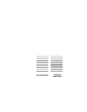
Figure 1. The algebraic energy sector coming from both algebraizations of potential (4) with $n=4$.

It is maybe worth to explore the relation between the two different algebraizations. It is known in the theory of Lie algebraic problems that under linear fractional transformations the Lie-algebraic character is preserved [20]. More specifically, a change of variable by a linear fractional transformation,

$$z=\frac{\alpha{\tilde{z}}+\beta}{\gamma{\tilde{z}}+\delta}\,,\qquad\alpha\delta-\beta\gamma=1,$$

together with an appropriate gauge transformation preserve the space $\mathcal{P}_{n}$ since

(16) $$p(z)\in\mathcal{P}_{n}(z)\mapsto\tilde{p}({\tilde{z}})=(\gamma{\tilde{z}}+\delta)^{n}p\left(\frac{\alpha{\tilde{z}}+\beta}{\gamma{\tilde{z}}+\delta}\right)\in\mathcal{P}_{n}({\tilde{z}})\,.$$

Moreover, if $T$ is Lie-algebraic and preserves $\mathcal{P}_{n}(z)$, then

(17) $$\tilde{T} = (-\gamma z+\alpha)^{-n}\,T\,(-\gamma z+\alpha)^{n}$$

is also Lie-algebraic and preserves $\mathcal{P}_{n}({\tilde{z}})$. We see thus that projective transformations do not change the $\operatorname{sl}(2)$ character, in fact they amount to a linear transformation of the generators of $\operatorname{sl}(2)$ [20]. However, from expressions (5),(6),(10) and (11) it follows that the relation between the two algebraic operators $T$ and $\hat{T}$ in the previous example is given by

(18) $$z = -\frac{(w-1)^{2}}{4w},$$

(19) $$T = w^{-n}\,\hat{T}\,w^{n},$$

which is not a projective transformation.

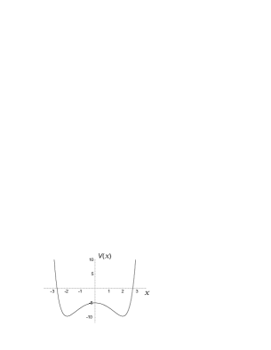
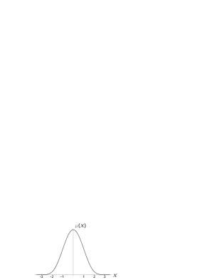
Potential $V(x)$	Gauge factor $\mu(x)$
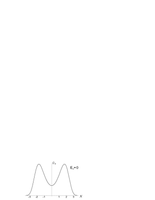
Ground state $\psi_{0}(x)$	Second excited state $\psi_{2}(x)$
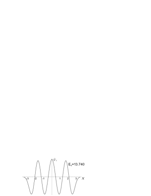
Fourth excited state $\psi_{4}(x)$	Sixth excited state $\psi_{6}(x)$

Figure 2. The four algebraic eigenfunctions obtained through $\operatorname{sl}(2)$ algebraization of potential (4) with $n=3$ and $A=-0.4$

We have performed an explicit computation to show a few of the algebraic eigenfunctions of the Hamiltonian (4). For illustrative purposes it suffices to fix the integer parameter $n$ to some low value. For the values $n=3$ and $A=-0.4$ the potential (4) has the shape of a double-well potential shown in Figure 2.

2.1. $\operatorname{sl}(2)$ algebraization

For $n=3$ the operator $T$ in (7) satisfies

$$T\,\mathcal{P}_{3}(z)\subset\mathcal{P}_{3}(z)$$

which allows to compute four algebraic eigenfunctions via the $\operatorname{sl}(2)$ algebraization. The action of $T$ relative to the canonical basis of $\mathcal{P}_{3}$ is given by the following $4\times 4$ matrix:

$$T\Big{|}_{\,\mathcal{P}_{3}}={\footnotesize\left(\begin{array}[]{cccc}0&-24A&0&0\\ 1/2&-8A&-16A&0\\ 0&3&-2-16A&-8A\\ 0&0&15/2&-6-24A\\ \end{array}\right)}.$$

For $A=-0.4$ we have calculated four algebraic eigenfunctions of (4) which have the form

(20) $$\psi_{2k}(x)=\mu(x)\,p_{k}(\sinh^{2}{\footnotesize\frac{x}{2})},\qquad k=0,1,2,3,$$

where $p_{k}\in\mathcal{P}_{3}(z)$ is one of the four eigen-polynomials of $T$ and the gauge factor $\mu(x)$ is given by (5). These four eigenfunctions have been plotted in Figure 2 along with their corresponding energies, which have been normalized so that the energy of the ground state is zero.

2.2. Exceptional module algebraization

From the second algebraization we know that the Schrödinger operator $H$ is conjugate via the change of variables (11) and gauge factor (10) to the operator $\hat{T}$ which preserves an exceptional polynomial module. For $n=3$ this space is spanned by

(21) $$\mathcal{E}^{(3,-1)}_{6}(w)=\left\langle-2-3w,(w+1)^{2},(w+1)^{3},(w+1)^{4},(w+1)^{5},(w+1)^{6}\right\rangle,$$

and the matrix of the action of $\hat{T}$ relative to this basis is

$$\hat{T}\Big{|}_{\,\mathcal{E}^{(3,-1)}_{6}}={\footnotesize\left(\begin{array}[]{cccccc}6-12A&-30A&0&0&0&0\\ 2&10-4A&8A&0&0&0\\ 0&-6&12&6A&0&0\\ 0&-4&-2&12+4A&4A&0\\ 0&0&-10&6&10+8A&2A\\ 0&0&0&-18&18&6+12A\\ \end{array}\right)}\,.$$

For the same value $A=-0.4$ we have calculated six algebraic eigenfunctions of the Hamiltonian (4) which have the form

(22) $$\psi_{k}(x)=\hat{\mu}(x)\,\hat{p}_{k}({\rm e}^{x}),\qquad k=0,1,2,3,4,6.$$

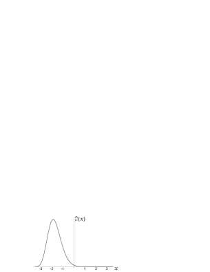
Potential $V(x)$	Gauge factor $\hat{\mu}(x)$
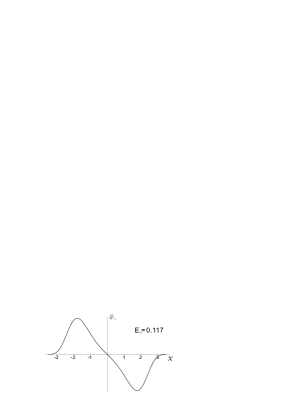
Ground state $\psi_{0}(x)$	First excited state $\psi_{1}(x)$
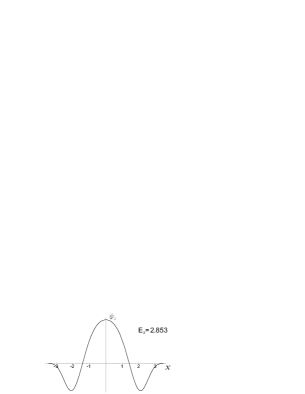
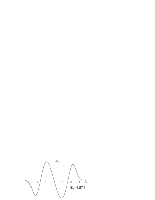
Second excited state $\psi_{2}(x)$	Third excited state $\psi_{3}(x)$
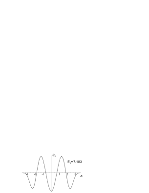
Fourth excited state $\psi_{4}(x)$	Sixth excited state $\psi_{6}(x)$

Figure 3. The six algebraic eigenfunctions obtained through the exceptional module algebraization of potential (4) with $n=3$ and $A=-0.4$

where $\hat{p}_{k}\in\mathcal{E}^{(3,-1)}_{6}$ is one of the six eigen-polynomials of $\hat{T}$ and the gauge factor $\hat{\mu}(x)$ is given by (10). These six algebraic eigenfunctions along with their energies are shown in Figure 3. The first thing to note is that we obtain all the even eigenfunctions from the $\operatorname{sl}(2)$ algebraization plus two extra odd eigenfunctions corresponding to the first and third excited states. However, the eigenfunction corresponding to the fifth excited state is not present in the algebraic sector. For arbitrary $n$ it seems that there is always a gap in the algebraic sector just below the highest energy in the exceptional module algebraization, [15]. Although all evidences show that this is true in the general case, there is yet no proof of this result.

3. A non-Lie algebraic quasi-exactly solvable potential

In the previous section we have seen how the exceptional module algebraization can provide more energy levels from a Lie-algebraic potential. In this Section we will show that some Schrödinger operators only admit an exceptional module algebraization and not the traditional $\operatorname{sl}(2)$ one. We can therefore construct new quasi-exactly solvable potentials on the line, which are not in the classifications of QES potentials in [20, 7], since those classifications deal only with potentials that admit an $\operatorname{sl}(2)$ algebraization. In this Section we show one first simple example of this phenomenon, postponing the full classification of these new potentials to a future publication,[19].

Consider the following Schrödinger operator:

(23) $$H=-D_{xx}+V(x)$$

with potential

(24) $$V(x)=A^{2}x^{6}+2ABx^{4}+\big{(}B^{2}+[(-1)^{p}-4n]A\big{)}x^{2}+4\frac{x^{2}-1}{(x^{2}+1)^{2}}.$$

If the last rational term were absent, this potential would be the well known quasi-exactly solvable sextic potential discussed for instance in [6]. The potential is always even, so its eigenfunctions will have well defined parity. However, as it happens with the sextic, only even or odd eigenfunctions but not both appear in the algebraic sector. This does not exclude in principle that other algebraizations exist in which both even and odd eigenfunctions are obtained. In fact, the choice of $p=0$ gives a potential with algebraic even eigenfunctions while $p=1$ corresponds to potentials with odd algebraic eigenfunctions. For arbitrary values of $A$ and $B$ the Hamiltonian does not preserve any finite dimensional subspace, but for the following values:

(25) $$A = \frac{a}{n-a}\left(a-\frac{(-1)^{p}}{2}\right),$$

(26) $$B = \frac{a}{n-a}\left(3a-2n+(-1)^{p}\big{(}\frac{n}{2a}-1\big{)}\right),$$

where $a$ is an arbitrary real parameter, the Hamiltonian $H$ admits an exceptional module algebraization. More specificallly, the transformation $T=\mu(x)^{-1}H\,\mu(x)$ with

(27) $$\mu(x) = \frac{x^{p}}{x^{2}+1}\,{\rm exp}\big{(}-\frac{A}{4}x^{4}-\frac{B}{2}x^{2}\big{)},\quad p=\{0,1\}$$

(28) $$w = x^{2}$$

transforms $H$ into the algebraic operator $T$ given by

$$T(w)=4\big{(}J_{4}+J_{5}-AJ_{6}\big{)}$$

up to an additive constant. The operators $J_{4}$, $J_{5}$ and $J_{6}$ are given by

(29) $$J_{4} = (w-1)D_{ww}+\big{(}a(w-1)-1\big{)}D_{w},$$

(30) $$J_{5} = D_{ww}+2\Big{(}a-\frac{1}{w-1}\Big{)}D_{w}-\frac{2a}{w-1},$$

(31) $$J_{6} = (w-1)\Big{(}w-1-\frac{n}{a}\Big{)}D_{w}-n(w-1),$$

and every one of them leaves invariant the exceptional module $\mathcal{E}_{n}^{(a,1)}(w)$ given by

(32) $$\mathcal{E}_{n}^{(a,1)}(w)=\big{\langle}1-a(w-1),(w-1)^{2},(w-1)^{3},\dots,(w-1)^{n}\big{\rangle}$$

The sextic potential (24) has eigenfunctions in $L_{2}(\mathbb{R})$ provided that $A<0$, or $A=0$ and $B<0$. This last case corresponds in fact to an exactly solvable potential, which can be obtained by a SUSY transformation from the harmonic oscillator [16]. The algebraic operator preserves in this last case an infinite flag of exceptional polynomial subspaces.

We show some explicit eigenfunctions of this potential corresponding to the even sector by setting $n=4$ and $p=0$. The matrix of the action of $T$ with respect to the basis (32) of $\mathcal{E}_{4}^{(a,1)}(w)$ is

$$T\Big{|}_{\,\mathcal{E}^{(a,1)}_{4}}={\footnotesize\left(\begin{array}[]{cccc}\frac{-15a^{2}-a+6}{a-4}&\frac{6a^{2}(1-2a)}{a-4}&0&0\\ -8&\frac{-19a^{2}+47a-10}{a-4}&\frac{4a(2a-1)}{a-4}&0\\ 0&4(4a-3)&\frac{-23a^{2}+79a-18}{a-4}&\frac{2a(2a-1)}{a-4}\\ 0&16&8(3a-4)&\frac{-27a^{2}+111a-26}{a-4}\\ \end{array}\right)}\,.$$

For $a=0.8$ the four polynomial eigenfunctions of $T$ are approximately

$$p_{0}(w) = 0.431+2.555w+3.543w^{2}+2.071w^{3}+0.325w^{4},$$

$$p_{1}(w) = 0.965+2.799w+2.681w^{2}+0.776w^{3}-0.055w^{4},$$

$$p_{2}(w) = 0.647+0.230w+0.369w^{2}-0.052w^{3}+0.0017w^{4},$$

$$p_{4}(w) = 0.329-0.538w+0.114w^{2}-0.008w^{3}+0.0001w^{4},$$

where polynomial $p_{k}$ has $k$ zeros. The corresponding energies are:

$$E_{0} = 0,$$

$$E_{2} = 6.058,$$

$$E_{4} = 11.148,$$

$$E_{8} = 15.129.$$

Therefore the four even eigenfunctions of (24) coming from the exceptional module algebraization are:

(33) $$\psi_{2k}(x)=\mu(x)\,p_{k}(x^{2}),\qquad k=0,1,2,4.$$

where the gauge factor $\mu(x)$ is given by (27) with $p=0$. For this choice of parameters $a$, $p$ and $n$ the potential, gauge factor and eigenfunctions have been plotted in Figure 4. We observe once again that we obtain eigenfunctions with zero, two, four and eight zeros, but not one with six zeros. For arbitrary $n$ the eigenfunction with $2n-2$ zeros would be missing form the algebraic sector. The calculations for the odd case are similar: setting $p=1$ in (24) we have calculated $n=4$ odd eigenfunctions which are shown in Figure 5.

4. Discussion

By means of two examples we provide further arguments to motivate the study of quasi-exactly solvable problems beyond the Lie algebraic approach. Even in the simplest case of one dimensional quantum mechanical problems the classifications performed in [7, 20] do not cover all quasi-exactly solvable potentials. Since Lie algebraic potentials are only a subclass of the potentials with partial algebraization of their spectrum, it would be desirable to find a precise mathematical characterization of the latter. This problem is related to the so called generalized Bochner problem [21], that of finding the most general differential operator that preserves a general finite dimensional space of polynomials. All the new quasi-exactly solvable potentials obtained recently are based on the exceptional modules, but other polynomial subspaces might exist which do not have a monomial basis and yet have a rich structure. In conclusion, the class of Hamiltonians with partial algebraization of their spectrum is larger than it was previously thought, and the new results call for new theoretical developments on this field.

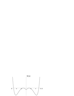
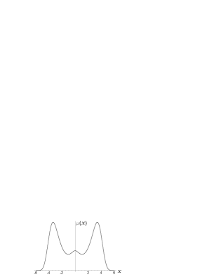
Potential $V(x)$	Gauge factor $\mu(x)$
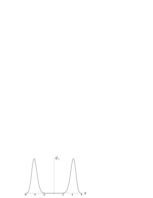
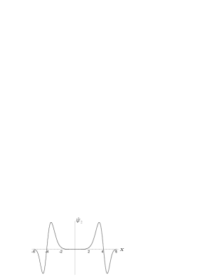
Ground state $\psi_{0}(x)$	Second excited state $\psi_{2}(x)$
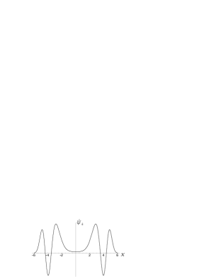
Fourth excited state $\psi_{4}(x)$	Eighth excited state $\psi_{6}(x)$

Figure 4. Four even eigenfunctions of the modified sextic potential (24) with $a=0.8$, $n=4$ and $p=0$, corresponding to the exceptional module algebraization.

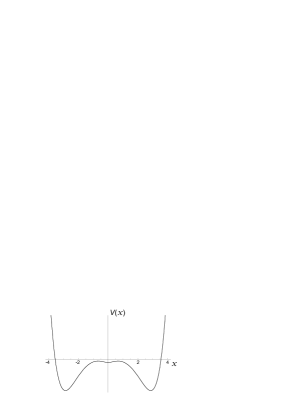
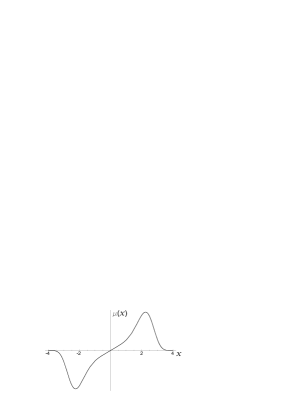
Potential $V(x)$	Gauge factor $\mu(x)$
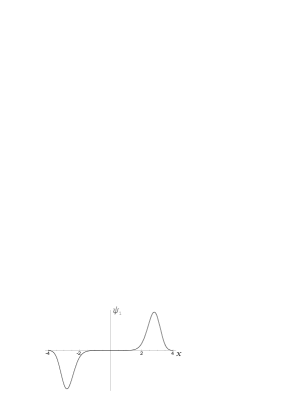
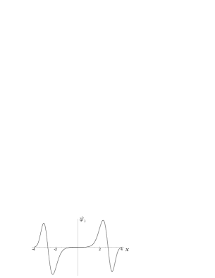
First excited state $\psi_{1}(x)$	Third excited state $\psi_{3}(x)$
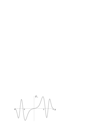
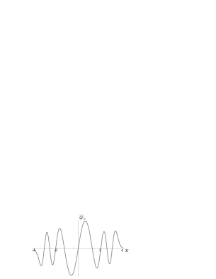
Fifth excited state $\psi_{5}(x)$	Ninth excited state $\psi_{9}(x)$

Figure 5. Four odd eigenfunctions of the modified sextic potential (24) with $a=0.8$, $n=4$ and $p=1$, corresponding to the exceptional module algebraization.

References

[1] S. Goshen and H. J. Lipkin, A simple independent
particle having collective properties, Ann. Phys. 6 (1959),
301-309.
[2] A. Bohm and A. O. Barut, Dynamical groups and mass
formula, Phys. Rev. 139 (1965), B1107-B1112.
[3] Y. Dothan, M. Gell-Mann and Y. Ne’ eman, Series
of hadron energy levels as representations of non-compact groups,
Phys. Lett. 17 (1965), 148-151.
[4] A. Bohm and Y. Ne’ eman, Dynamical groups and
spectrum generating algebras in : Dynamical Groups and Spectrum
Generating algebras, A. Bohm, Y. Ne’ eman and A.O. Barut, eds.,
World Scientific, Singapore, 1988. pp. 3-68.
[5] F. Iachello and R. D. Levine, Algebraic Theory
of Molecules, Oxford University Press, Oxford, 1995.
[6] M. Shifman and A. Turbiner, Quantal problems with partial algebraization of the spectrum, Commun. Math. Phys. 126 (1989) 347-365.
[7] A. Turbiner, Quasi-exactly-solvable problems and
algebra, Commun. Math. Phys. 118 (1988),
467-474.
[8] A. Ushveridze, Quasi-exactly-solvable models in quantum mechanics, Institute of Physics Publishing: Bristol 1994.
[9] A. Ushveridze, Quasi-exactly-solvable models in quantum
mechanics, Sov. J. Part Nucl. 20 (1989), 504-528.
[10] R. Milson, On the construction of quasi-exactly
solvable Schrodinger operators on homogeneous spaces, J. Math.
Phys. 36 (1995), 6004–6027.
[11] A. González-López, N. Kamran, and P.J. Olver, Quasi-exactly
solvable Lie algebras of differential operators in two complex
variables J. Phys. A 24 (1991), 3995–4008.
[12] D. Gómez-Ullate, A. González-López, and M.A. Rodríguez,
Exact solutions of an elliptic Calogero-sutherland model,
Phys. Lett. B511 (2001), 112-118.
[13] D. Gómez-Ullate, A. González-López, and
M. A. Rodríguez, New algebraic quantum many-body
problems, J. Phys. A 33 (2000), 1-31.
[14]
G. Post and A. Turbiner, Classification of linear
differential operators with an invariant subspace of monomials,
Russian J. Math. Phys. 3 (1995), 113-122.
[15]
D. Gómez-Ullate, N. Kamran, and R. Milson, Quasi-exact
solvability and the direct approach to invariant subspaces, J.
Phys. A 38 (2005), 2005-2019.
[16]
D. Gómez-Ullate, N. Kamran, and R. Milson, The Darboux
transformation and algebraic deformations of shape-invariant
potentials, J. Phys. A 37 (2004), 1789-1804.
[17]
D. Gómez-Ullate, N. Kamran, and R. Milson, Supersymmetry
and algebraic Darboux transformations, J. Phys. A 37
(2004), 10065-100078.
[18] A. González-López and T. Tanaka T, A novel
multi-parameter family of quantum systems with partially broken -fold
supersymmetry J. Phys. A 38 (2005), 5133-5157
[19]
D. Gómez-Ullate, N. Kamran, and R. Milson, in preparation.
[20] A. González-López, N. Kamran and P. J. Olver,
Normalizability of one-dimensional quasi-exactly solvable
Schrödinger operators, Commun. Math. Phys. 153 (1993)
117–146.
[21] A. Turbiner, Lie-algebras and linear operators with invariant
subspaces in “Lie algebras, cohomology, and new applications to
quantum mechanics”, N. Karmran and P. J. Olver eds., 263–310,
Contemp. Math., 160, AMS, 1994.