Driving convection by a temperature gradient or a heat current

Abstract

Bifurcation properties, stability behavior, dynamics, and the heat transfer of convection structures in a horizontal fluid layer that is driven away from thermal equilibrium by imposing a vertical temperature difference are compared with those resulting from imposing a heat current. In particular oscillatory convection that occurs in binary fluid mixtures in the form of travelling and standing waves is determined numerically for the two different driving mechanisms. Conditions are elucidated under which current driven convection is stable while temperature driven convection is unstable.

Many nonlinear dissipative systems that are driven away from thermal equilibrium show selforganization out of an unstructured state: A structured one appears when the driving exceeds a critical threshold CH93 . The driving might be realized by imposing a field gradient across the system — e.g., a voltage difference across a semiconductor semicond or a liquid crystal liquid-crystal , a temperature difference across a fluid layer BPA00 , or a concentration difference in a physical PCSN94 , chemical K03 , or biological CDFSTB03 system — which drives a current. Or, alternatively, a current might be injected at one side of the system AhlersQT ; WKPS85 ; MS86 . Now the question is, whether and how the dissipative structures that form in response to these two different driving mechanisms are related to each other concerning their dynamics, their structure, their stability behavior, and their bifurcation properties.

We have investigated this question numerically for the case of convection in a horizontal layer of a binary fluid like, e.g., ethanol-water early-exp . Unlike one-component fluids like pure water, this system shows a surprisingly rich variety of different convection structures already at small driving CH93 ; PL84 ; LBBFHJ98 . There are spatially extended states of stationary convection rolls and of temporally oscillating roll patterns in the form of traveling waves (TWs) and of standing waves (SWs) that bifurcate out of the quiescent fluid state. In addition there are also spatially localized traveling wave states that compete with extended convection structures.

Here, we focus on convection in the form of straight parallel rolls as they occur, e.g., in narrow channels with roll axes perpendicular to the long side walls. We have solved the appropriate hydrodynamic field equations PL84 ; LL87 with a finite-differences method BLKS95I in a vertical $x-z$ cross section through the rolls perpendicular to their axes thus ignoring effects that come from field variations along the roll axes PL84 ; CJT97 ; AlBa04 .

Calculations were done for ethanol-water parameters, Lewis number $L$=0.01 and Prandtl number $\sigma$=10. Results are presented here for two different separation ratios $\psi$=-0.03 and $\psi$=-0.1 coupling for which TW and SW solutions bifurcate subcritically out of the quiescent fluid state via a common Hopf bifurcation. Our findings concerning the above posed questions are representative also for TWs and SWs at stronger, i.e., more negative Soret coupling strength $\psi$.

The horizontal boundaries at top ($z$=1) and bottom ($z$=0) are no-slip, impermeable, and perfectly heat conducting, thus enforcing the absence of lateral temperature gradients there. Sapphire or copper plates provide a good experimental approximation. Two different experimentally realizable horizontal boundary conditions (bc) for the temperature are explored here: (i) Dirichlet bc of fixed temperatures (constant in space and time) at $z$=0 and $z$=1 with a difference of $\Delta T$ between them and (ii) von Neumann bc of fixed total vertical heat current at $z$=0 and Dirichlet bc of fixed temperature at $z$=1. At the impermeable boundaries the vertical concentration current vanishes and consequently the local vertical heat current reduces there to $-\partial_{z}T$ LL87 . Note that we impose in case (ii) the horizontal mean

$$Q=-\overline{\partial_{z}T|_{z=0}}$$ (1)

of the heat current at the lower side of the fluid layer so that the total heat current injected into it is a constant. We shall identify the driving conditions of case (i) by TT for short and those of case (ii) by QT.

Laterally we impose for all fields periodic bc with wavelength $\lambda$=2. This is roughly the critical one for onset of oscillatory convection. Moreover, it is often seen also in nonlinear convection with rolls of about circular shape. Finally, to determine SW solutions that are unstable against horizontal mirror symmetry breaking phase propagation we enforce horizontal mirror symmetry, say, at $x$=0 thereby fixing the phase MDL04 .

As control parameter measuring the strength of the driving we use in the TT case the relative deviation

$$\epsilon=\Delta T/\Delta T_{c}-1$$ (2)

from the critical temperature difference $\Delta T_{c}$ for onset of convection. The driving in case QT is measured by the relative deviation

$$\rho=Q/Q_{c}-1$$ (3)

from the critical imposed heat current.

We shall discuss first TW convection and then SW solutions. In Figs. 1 and 2 we show for two different $\psi$ the bifurcation diagrams of nonlinear relaxed TW states: (i) current $Q$ as a function of $\epsilon$ for TT driving and (ii) temperature difference $\Delta T$ versus $\rho$ for the QT case. Note that $Q$ as well as $\Delta T$ are constant for TWs. The diagonal line shows the linear diffusive relation $Q_{cond}/Q_{c}=\Delta T_{cond}/\Delta T_{c}$ of the quiescent conductive state. It loses stability via a Hopf bifurcation at $\Delta T_{c}$ or $Q_{c}$, respectively. After increasing the driving slightly beyond this threshold transient growth of oscillatory convection occurs with increasing $Q$ for the TT case. For QT conditions $\Delta T$ decreases since convection cools the lower boundary. Initially, the oscillations have the Hopf frequency. But finally, the TT transient ends in a stationary convection state since the TW branch terminates with zero frequency in a stationary solution branch already below $\epsilon$=0 for our $\psi$’s rstar . On the other hand, the QT growth transient ends in a relaxed nonlinear TW (lower part of Figs. 1 and 2).

The curves of $Q/Q_{c}$ versus $\epsilon$ and of $\Delta T/\Delta T_{c}$ versus $\rho$ in Figs. 1 and 2 are reflections of each other at the diagonal, bisecting conduction line. Note, however, that the transients and the stability ranges of the relaxed TWs are different. Concerning the latter, for example, the hysteresis interval in $\rho$ for QT is significantly smaller than the one in $\epsilon$ for TT since a large portion of unstable TT generated TWs below onset gets stabilized under QT driving.

In Fig. 3 we show for the TWs of Fig. 1 bifurcation diagrams of Nusselt number $N$, reduced frequency $\omega/\omega_{c}$, and squared maximal vertical velocity $w_{max}^{2}$ versus the respective control parameters. The Nusselt number

$$N=Q/Q_{cond}=(Q/Q_{c})\Delta T_{c}/\Delta T$$ (4)

provides the relation

$$\rho=(1+\epsilon)N-1$$ (5)

between equivalent control parameters $\epsilon$ and $\rho$ corresponding to reflection at the conductive diagonal in Figs. 1 and 2: TWs that are generated by TT or QT driving at $\epsilon$- and $\rho$-values related by (5) have the same spatiotemporal properties, e.g., the same $N,\omega,w_{max}$ as indicated by the symbols in Fig. 3. Their stability, however, might differ.

Eq. (5) yields also the relation

$$\partial_{\rho}A=\partial_{\epsilon}A/[N+(1+\epsilon)\partial_{\epsilon}N]$$ (6)

between the slopes $\partial_{\rho}A(\rho)$ and $\partial_{\epsilon}A(\epsilon)$ in the QT and TT bifurcation diagrams of any order parameter $A$ (say, $N,\omega,w_{max}^{2},etc)$ versus $\rho$ or $\epsilon$, respectively. Hence, the QT bifurcation becomes already tricritical, i.e., it changes from backwards to forwards when the initial slope $s=\partial_{\epsilon}N(\epsilon=0)$ of the TT Nusselt number increases beyond $-1$. In other words, all TT driven backwards bifurcating unstable TWs for which $s>-1$ can be stabilized by switching over to QT driving.

Note that the relations (5) and (6) hold also for any stationary convection solution so that the bifurcation diagrams of $Q/Q_{c}$ versus $\epsilon$ and of $\Delta T/\Delta T_{c}$ versus $\rho$ are reflections of each other. Thus, the stabilization effect of QT driving holds also for any stationary convection that bifurcates backwards with TT Busse . The (stability) properties of forward bifurcating stationary convection remain unchanged when using QT instead of TT conditions.

In the remainder of this letter we dicuss SW convection. Under TT (QT) driving the heat current $Q$ (temperature difference $\Delta T$) oscillates with twice the SW frequency SWoscillations . So, in Figs. 1 and 2 we show bifurcation diagrams of the time averages $\left<Q\right>/Q_{c}$ and $\left<\Delta T\right>/\Delta T_{c}$, respectively. Like for TWs, QT conditions have a stabilizing effect also on SWs. Note, however, that the two SW solution branches in these Figs. are not reflections of each other at the conduction diagonal. Their spatiotemporal properties differ and the relation $\left<\rho\right>=(1+\epsilon)\left<N\right>-1$ provides only an approximate equivalence between the bifurcation diagrams of the order parameters in Fig. 4 and 5. For example, the SWs marked by symbols in Fig. 5 have the same frequency. But $w_{max}$ differs slightly and so does $\left<N\right>$ — i.e., $\left<Q/Q_{c}\right>\Delta T_{c}/\Delta T$ for TT driving in comparison with $(Q/Q_{c})\left<\Delta T_{c}/\Delta T\right>$ for QT driving. Also the oscillations of the flow differ slightly [Fig. 6(c)]. On the other hand, the oscillation profile of $Q(t)$ differs significantly from the one of $\Delta T(t)$ [Fig. 6(a)] and also the profile of $N_{TT}(t)$ differs from the one of $N_{QT}(t)$ [Fig. 6(b)].

In summary: Driving convection with a fixed heat current can stabilize SW, TW, and stationary states that bifurcate backwards and that are unstable with imposed temperature difference. However, irrespective of their stability relaxed TWs for the two driving mechanisms are simply related to each other. The same holds for stationary solutions. But the time evolution of, say, growth transients differ in general. Also SW oscillations driven by a constant field gradient differ from those resulting from constant current driving. It would be interesting to see how far these different conditions influence the spatio temporal properties of convection structures with more complex dynamics.

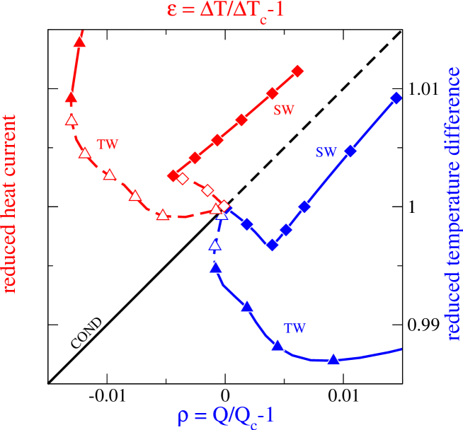
Figure 1: (color online) Bifurcation diagrams of heat current and temperature difference for oscillatory convection at $\psi=-0.03$ subject to different bc. The upper left (lower right) part shows $Q/Q_{c}$ ($\Delta T/\Delta T_{c}$) for TT (QT) driving versus $\epsilon$ ($\rho$) on the upper (lower) abscissa. For SWs the time averages $\left<Q\right>/Q_{c}$ and $\left<\Delta T\right>/\Delta T_{c}$, respectively, are plotted. The bisecting line marks the quiescent conductive state. Full (dashed) lines and filled (open) symbols denote stable (unstable) states. SW solutions were obtained with phase pinning conditions; otherwise they are completely unstable.

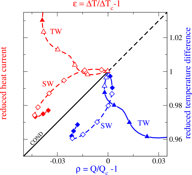
Figure 2: (color online) Bifurcation diagrams of heat current and temperature difference as in Fig. 1. Here, however, for $\psi=-0.1$.

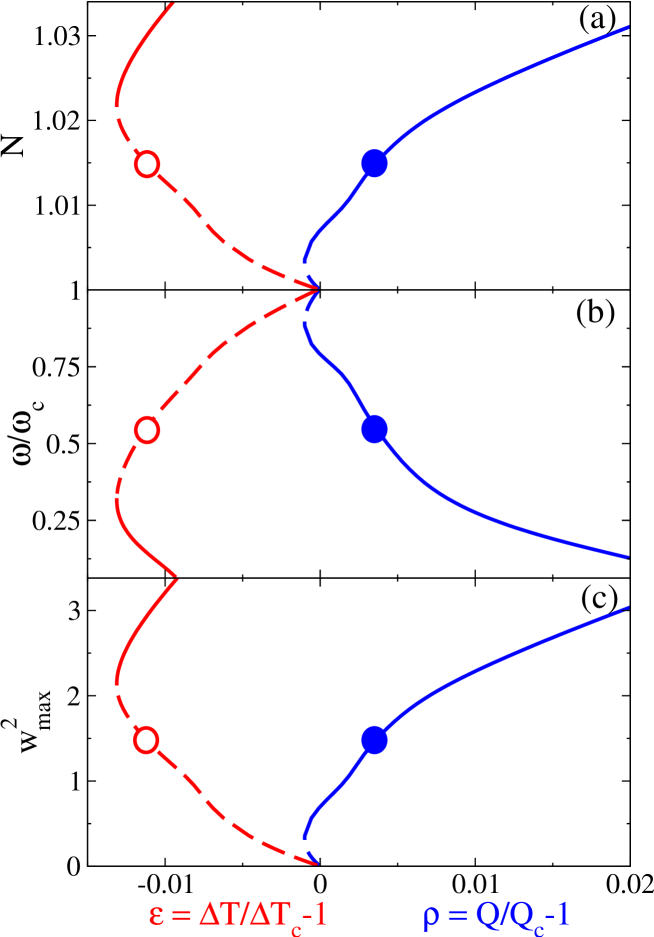
Figure 3: (color online) TW bifurcation diagrams: (a) Nusselt number $N$, (b) reduced oscillation frequency $\omega/\omega_{c}$, and (c) squared maximal vertical velocity $w_{max}^{2}$ for the TWs of Fig. 1 with $\psi=-0.03$. The left and right curves refer to TT and QT driving, respectively. Full (dashed) lines denote stable (unstable) TWs. Symbols identify examples of equivalent TWs for equivalent control parameters $\epsilon$ and $\rho$.

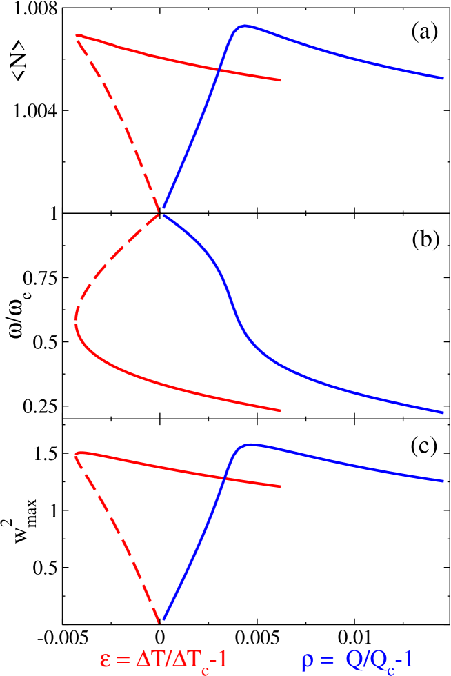
Figure 4: (color online) SW bifurcation diagrams: (a) time averaged Nusselt number $\left<N\right>$, (b) reduced oscillation frequency $\omega/\omega_{c}$, and (c) squared maximal vertical velocity $w_{max}^{2}$ for the SWs of Fig. 1 with $\psi=-0.03$. The left and right curves refer to TT and QT driving, respectively. Full (dashed) lines denote stable (unstable) SWs.

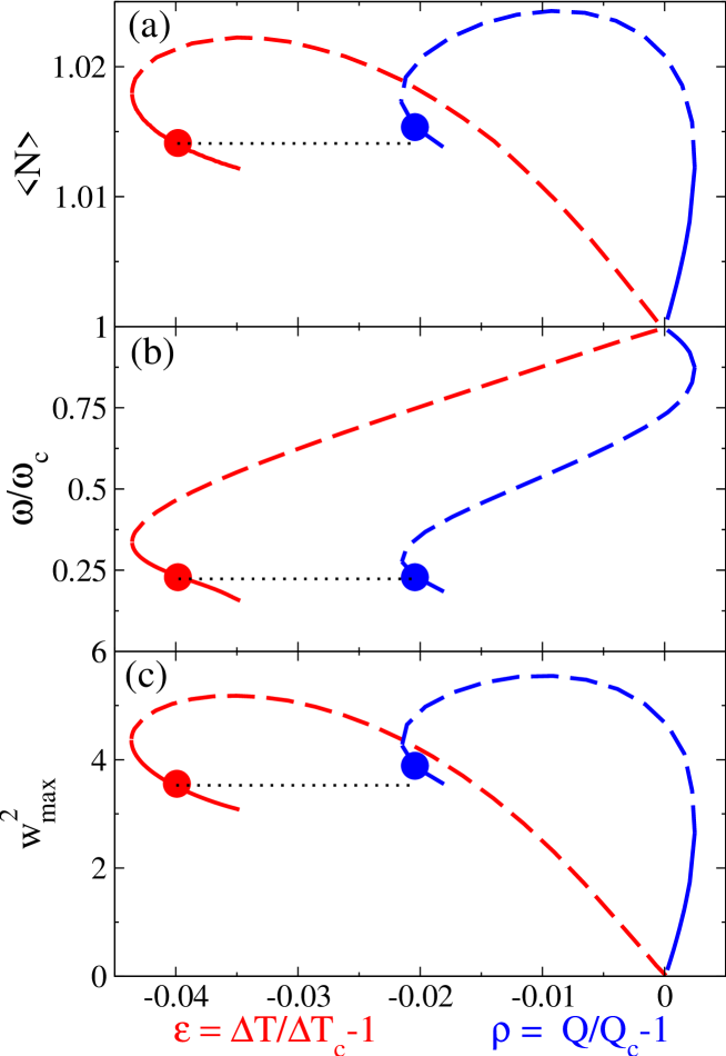
Figure 5: (color online) SW bifurcation diagrams as in Fig. 4 but for the SWs of Fig. 2 with $\psi=-0.1$. Symbols identify examples of SWs with the same frequency.

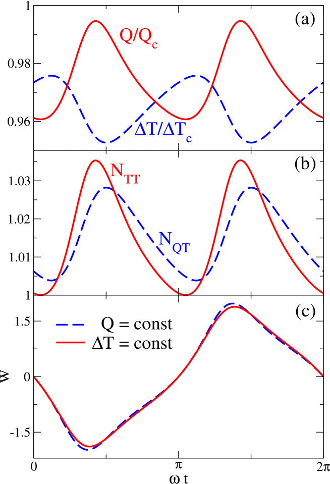
Figure 6: (color online) Oscillation profiles of the SWs marked in Fig. 5 by symbols. (a) Current and temperature oscillation subject to TT and QT driving, respectively. (b) Nusselt numbers $N_{TT}(t)=[Q(t)/Q_{c}]\Delta T_{c}/\Delta T=Q(t)/Q_{cond}$ and $N_{QT}(t)=(Q/Q_{c})[\Delta T_{c}/\Delta T(t)]=\Delta T_{cond}/\Delta T(t)$. (c) Vertical velocity $w$ at midheight between two rolls.

References

- (1) M. C. Cross and P. C. Hohenberg, Rev. Mod. Phys. 65, 851 (1993); and references cited therein.
- (2) E. Schöll, F. J. Niedernostheide, J. Parisi, W. Prettl, and H.G. Purwins, in Evolution of structures in dissipative continuous systems, edited by F. H. Busse and S. C. Müller, Lecture Notes in Physics, m55 (Springer, Berlin, 1998), p. 446; E. Schöll, Nonlinear Spatio-Temporal Dynamics and Chaos in Semiconductors, (Cambridge University Press, Cambridge, 2001); and references cited therein.
- (3) Pattern Formation in Liquid Crystals, edited by A. Buka and L. Kramer, (Springer, Berlin, 1996).
- (4) E. Bodenschatz, W. Pesch, and G. Ahlers, Annu. Rev. Fluid Mech. 32, 709 (2000).
- (5) A. A. Predtechensky, W. D. McCormick, J. B. Swift, Z. Noszticzius, and H. L. Swinney, Phys. Rev. Lett. 72, 218 (1994); N. Tsitverblit, Phys. Lett. A 329, 445 (2004).
- (6) Y. Kuramoto, Chemical Oscillations, Waves and Turbulence, (Courier Dover Publications , 2003).
- (7) S. Camazine, J. L. Deneubourg, N. R. Franks, J. Sneyd, G. Theraula, and E. Bonabeau, Self-Organization in Biological Systems, (Princeton University Press, 2003).
- (8) G. Ahlers, Phys. Rev. Lett. 33, 1185 (1974); R. P. Behringer and G. Ahlers, J. Fluid Mech. 125, 219 (1982); G. Ahlers and I. Rehberg, Phys. Rev. Lett. 56, 1373 (1986).
- (9) R. W. Walden, P. Kolodner, A. Passner, and C. M. Surko, Phys. Rev. Lett. 55, 496 (1985).
- (10) E. Moses and V. Steinberg, Phys. Rev. A 34, 693 (1986).
- (11) Early experiments done with an isopropanol-water mixture in two different set-ups showed different hysteresis loops in Schmidt-Milverton plots of temperature difference (on the ordinate) versus heat current (on the abscissa) depending on which of the two was imposed VP84 .
- (12) D. Villers and J. K. Platten, J. Non-Equilib. Thermodyn. 9, 131 (1984).
- (13) J. K. Platten and J. C. Legros, Convection in Liquids, (Springer, Berlin, 1984).
- (14) M. Lücke, W. Barten, P. Büchel, C. Fütterer, St. Hollinger, and Ch. Jung, in Evolution of Structures in Dissipative Continuous Systems, edited by F. H. Busse and S. C. Müller, Lecture Notes in Physics, m55 (Springer, Berlin,1998), p. 127.
- (15) L. D. Landau and E. M. Lifshitz, Fluid Mechanics, (Pergamon Press, Oxford, 1987).
- (16) W. Barten, M. Lücke, M. Kamps, and R. Schmitz, Phys. Rev. E 51, 5636 (1995).
- (17) A. Alonso and O. Batiste, Theoret. Comput. Fluid Dynamics 18, 239 (2004).
- (18) Ch. Jung, (Ph.D. thesis, Universität des Saarlandes, 1997).
- (19) For 1.4 weight % of ethanol mixed into water at the separation ratio measuring the Soret coupling strength between temperature and concentration gradients is KWM88 ; CJT97 .
- (20) P. Kolodner, H. L. Williams, and C. Moe, J. Chem. Phys. 88, 6512 (1988).
- (21) P. Matura, D. Jung, and M. Lücke, Phys. Rev. Lett. 92, 254501 (2004).
- (22) St. Hollinger and M. Lücke, Phys. Rev. E 57, 4238 (1998).
- (23) Pure fluids with temperature dependent material parameters that are showing a stationary backwards bifurcation for TT driving were predicted B67 to allow oscillations under QT conditions. But we did not find such a behavior in our system.
- (24) F. H. Busse, J. Fluid Mech. 28, 223 (1967).
- (25) For TT driving the laterally integrated currents at and oscillate in a SW in phase as a consequence of a mirror-glide symmetry LBBFHJ98 ; MDL04 : holds for the temperature deviation from the mean. For QT conditions the temperature oscillates almost in antiphase to the current at .