Breakup of Shearless Meanders and “Outer” Tori in the Standard Nontwist Map

Abstract

The breakup of shearless invariant tori with winding number $\omega=[0,1,11,1,1,\ldots]$ (in continued fraction representation) of the standard nontwist map is studied numerically using Greene’s residue criterion. Tori of this winding number can assume the shape of meanders (folded-over invariant tori which are not graphs over the $x$-axis in $(x,y)$ phase space), whose breakup is the first point of focus here. Secondly, multiple shearless orbits of this winding number can exist, leading to a new type of breakup scenario. Results are discussed within the framework of the renormalization group for area-preserving maps. Regularity of the critical tori is also investigated.

In recent years nontwist maps, area-preserving maps that violate the twist condition locally in phase space, have been the subject of several studies in physics and mathematics. These maps appear naturally in a variety of physical models. An important problem is the understanding of the breakup of invariant tori, which correspond to transport barriers in the physical model. We conduct a detailed study of the breakup of two types of invariant tori that have not been analyzed before.

I Introduction

We consider the standard nontwist map (SNM) $M$ as introduced in Ref. Del-Castillo-Negrete and Morrison, 1993,

$$x_{n+1} = x_{n}+a\left(1-y^{2}_{n+1}\right)$$

$$y_{n+1} = y_{n}-b\sin\left(2\pi x_{n}\right)\,,$$ (1)

where $(x,y)\in{\mathbb{T}}\times{\mathbb{R}}$ are phase space coordinates and $a,b\in{\mathbb{R}}$ are parameters. This map is area-preserving and violates the twist condition, $\partial x_{n+1}(x_{n},y_{n})/\partial y_{n}\neq 0$, along a curve in phase space. Although the SNM is not generic due to its symmetries, it captures the essential features of nontwist systems with a local, approximately quadratic extremum of the winding number profile.

Nontwist maps are low-dimensional models of many physical systems, as described in Refs. Wurm et al., 2005; Apte et al., 2003; Del-Castillo-Negrete et al., 1996. Of particular interest from a physics perspective is the breakup of invariant tori (which we alternatively call invariant curves), consisting of quasiperiodic orbits with irrational winding number (see Appendix), that often correspond to transport barriers in the physical system.

One important characteristic of nontwist maps is the existence of multiple orbit chains of the same winding number. For the SNM, in particular, the symmetry $S(x,y)=(x+1/2,-y)$ guarantees that whenever an orbit chain of a certain winding number exists, a second chain with the same winding number can be found.

Changing the map parameters $a$ and $b$ causes bifurcations of periodic orbit chains with the same winding number. Orbits can undergo stochastic layer reconnection (“separatrix” reconnection), or they can collide and annihilate. The simplest reconnection-collision scenarios, which involve sequences of collisions between elliptic and hyperbolic orbits of a single pair of periodic orbit chains with the same winding number, have been known since early study of nontwist systems.Howard and Hohs (1984) In the SNM, two standard scenarios can be distinguished that describe, respectively, the reconnection-collision sequence for a pair of either even or odd-period orbit chains. A detailed review of these scenarios, as well as a discussion of earlier studies of reconnection-collision phenomena in theory and experiments, can be found in Ref. Wurm et al., 2005.

As recently reported,Wurm et al. (2005) even the simple, non-generic SNM can have more than two orbit chains of the same winding number, and thus reconnection-collision scenarios are more intricate than previously expected. To illustrate this, two stages of the odd-period standard scenario are shown in Fig. 1. Each of the winding number profiles exhibits two peaks at or somewhat below the winding number of the colliding odd-period orbit, which is marked by the dashed vertical line. Between the peaks lies a recess, i.e., for any winding number between the lowest value of the recess and the peak values, e.g., the value marked by dotted verticals, four (or more) orbits of that winding number traverse the $x=0.5$ symmetry line. Similar observations can be made for other symmetry lines. Therefore, whenever a periodic orbit is studied with winding number inside the recess associated with a major odd-period orbit collision, complicated reconnection-collision scenarios are possible, which were called non-standard scenarios in Ref. Wurm et al., 2005.

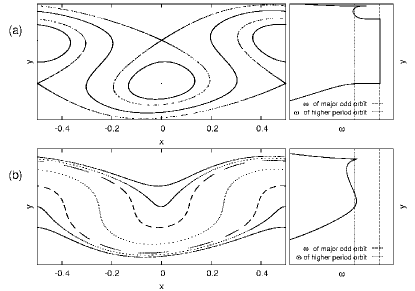
Figure 1: Phase space (left) and winding number profile along $x=0.5$ (right) of two stages of odd-period standard scenario. The $y$-ranges of all plots are identical. Parameters were chosen (a) slightly before collision and (b) slightly after collision of two major odd-period orbit chains (winding number marked by dashed lines).

When two quasiperiodic orbits collide, the winding number profile shows a local extremum and the orbit at collision is referred to as the shearless curve. In previous studies of the SNM only the shearless curves invariant under the full symmetry group $\cal G$ of the SNM (composed of the symmetry $S$ as well as the involutions $I_{1}$ and $I_{2}$) have been considered. However, as seen in Fig. 1(b), in addition to the central extremum (here a minimum) in the winding number profile, other shearless curves (here marked by the two outer peaks) may exist. Figure 1(a) also exhibits peaks, but since the plateau and spike are associated with an elliptic point and the invariant manifolds of hyperbolic points, respectively, rather than quasiperiodic orbits, they do not qualify as shearless curves. From now on, we will refer to the $\cal G$-invariant curve as the “central shearless curve” and to others as “outer shearless curves.” Since the breakup of outer shearless curves has not been studied so far, this will be the focus of our investigation in Sec. IV.

Another consequence of the violation of the twist condition is the occurrence of meanders, quasiperiodic orbits that are “folded over”, i.e., not graphs $y(x)$. Whereas Birkhoff’s theorem states that such curves cannot exist in twist maps, they can occur in nontwist maps. In the SNM, meanders appear between (in parameter space) the reconnection and collision of odd-period orbits.Petrisor (2001) Figure 1(a) shows an example, whereas in Fig. 1(b), the meander has changed to a graph again. As seen in Fig. 1(a), the region in which meanders are found corresponds to a recess in the winding number profile. However, the converse is not true: Fig. 1(b) shows an example where meanders are absent, but still a recess in the winding number profile is observed. To our knowledge, the breakup of meanders has not been studied previously.

The paper is organized as follows. In Sec. II we review previous results about the SNM relevant to this investigation. Section II.1 contains a brief discussion of the parameter space of the SNM, in particular the details of where the scenarios studied in this paper occur. Section II.2 contains an account of how Greene’s residue criterion is used for detecting the breakup of critical invariant tori. In Sec. III we discuss the results for the breakup of the central shearless meander of winding number $\omega=[0,1,11,1,1,\ldots]$ (in continued fraction representation), while in Sec. IV we consider the breakup of the outer shearless tori of the same winding number. Questions of regularity of these critical tori and a comparison with previous results are addressed in Sec. V. Finally, Sec. VI contains our conclusion and a discussion of open questions. Basic definitions are given in the Appendix.

II Background

II.1 Parameter space overview

In order to identify the parameter regions where the bifurcations described in Sec. I occur, various parameter space curves can be computed (usually numerically). Collisions of periodic orbits are described by the bifurcation curves introduced in Ref. Del-Castillo-Negrete et al., 1996 and generalized in Ref. Wurm et al., 2005. Reconnections do not occur precisely on parameter space curves (see, e.g., Ref. Apte et al., 2006), but within a finite range of parameters; however, the range is usually small enough that the method of Ref. Petrisor, 2002 (implemented in Ref. Wurm et al., 2004) yields curves that represent a good approximation of the reconnection thresholds for odd-period orbits. For even-period orbits, reconnection coincides with the collision of hyperbolic orbits.

By numerically computing the branching points at which bifurcation curves for various higher periodic orbits split up into several branches below a major odd-period orbit collision, one obtains a good estimate of the parameter region for which multiple orbit chains exist. For an extensive discussion of these curves and their computation see Ref. Wurm et al., 2005.

An overview of parameter space with thresholds for several examples of low-period orbits is shown in Fig. 2. Higher orbit branching points, bifurcation curves, and approximate reconnection thresholds are shown for the odd-period orbits 2/3 and 1/1. Meanders occur between reconnection and collision; a recess in winding number profile is encountered in the region limited by branching points and bifurcation curve. For even-period orbits with winding number 1/2, 5/6, and 11/12, only bifurcation curves are shown, since even-period orbits do not induce branching and reconnections coincide with collisions. Of the corresponding winding numbers, no orbits exist above the highest (in $b$) bifurcation curve and two orbit chains are found below the lowest one; in between various numbers of orbits exist on each symmetry line. In addition, the figure also contains the ragged breakup boundary, introduced in Ref. Shinohara and Aizawa, 1997, above which the central shearless orbits have become chaotic. We further indicate points (by triangles) for which the breakup of the central shearless curve has been studied in detail in the past (see Refs. Del-Castillo-Negrete et al., 1996; Wurm, 2002; Apte et al., 2003, 2005; Apte, 2004) as well as the two points investigated in this paper: The central meander from Sec. III is shown as a solid circle ($\bullet$), the outer shearless curves from Sec. IV as an empty circle ($\odot$). Note that all breakup points for central shearless tori are located on the breakup boundary, whereas the outer shearless curves break up at smaller parameter values.

Figure 2: Parameter space overview of SNM, with higher orbit branching points, bifurcation (collision) curves, and approximate reconnection thresholds for odd-period orbits 2/3 and 1/1. Bifurcation curves for even-period orbits 1/2, 5/6, and 11/12 and the breakup boundary for the central shearless tori are indicated. New points are marked by two circles. ($\odot$ denotes outer shearless curve, all others are central ones.)

The winding number investigated here was chosen such that the central shearless curve is a meander, i.e., the point $\bullet$ is located between the 1/1 reconnection and collision thresholds, and that multiple orbit chains and hence multiple shearless curves can occur, i.e., the point $\odot$ is located to the right of the 1/1 branching threshold. This can be ensured by picking a winding number close to a periodic orbit, here $11/12$, whose bifurcation curve both branches due to a nearby major odd-period orbit, and has one branch crossing a collision threshold of this major odd-period orbit before crossing the breakup boundary.

II.2 Greene’s residue criterion

Whereas the breakup boundary in Fig. 2 provides a rough estimate of the parameter values at which central shearless tori break, a significantly more precise tool for studying the breakup of a particular torus with given winding number is provided by Greene’s residue criterion, originally introduced in the context of twist maps.Greene (1979) This method relies on the numerical observation that the breakup of an invariant torus with irrational winding number $\omega$ is determined by the stability of nearby periodic orbits. Some aspects of the validity of this criterion have been proved for nontwist maps.Delshams and de la Llave (2000)

To study the breakup, one considers a sequence of periodic orbits with winding numbers $m_{i}/n_{i}$ converging to $\omega$, $\lim_{i\rightarrow\infty}m_{i}/n_{i}=\omega$. The sequence converging the fastest, and hence the most commonly used one, consists of the convergents of the continued fraction expansion of $\omega$, i.e., $m_{i}/n_{i}=[a_{0},a_{1},\ldots,a_{i}]$, where

$$\omega=[a_{0},a_{1},a_{2},\ldots]=a_{0}+\cfrac{1}{a_{1}+\cfrac{1}{a_{2}+\ldots}}.$$ (2)

The stability of the corresponding orbits can be expressed through their residues, $R_{i}=[2-{\rm Tr}(DM^{n_{i}})]/4$, where ${\rm Tr}$ is the trace and $DM^{n_{i}}$ is the linearization of the $n_{i}$ times iterated map about the periodic orbit: An orbit is elliptic for $0<R_{i}<1$, parabolic for $R_{i}=0$ and $R_{i}=1$, and hyperbolic otherwise. The convergence or divergence of the residue sequence associated with the chosen periodic orbit sequence then determines whether the torus exists or not, respectively:

• $\lim_{i\rightarrow\infty}|R_{i}|=0$ if the torus of winding number $\omega$ exists.

• $\lim_{i\rightarrow\infty}|R_{i}|=\infty$ if the torus of winding number $\omega$ is destroyed.

At the breakup itself, various scenarios can be encountered, depending on the class of maps and invariant torus under consideration.

For twist systems, this criterion has been used to study the breakup of noble invariant tori in the standard (twist) map, i.e., orbits with winding numbers that have a continued fraction expansion tail of 1’s (see, e.g., Refs. Greene, 1979; MacKay, 1982, 1983). It was found that at the point of breakup the sequence of residues converges to either $R_{\infty}\approx 0.25$ or a three-cycle containing $0.25\ldots$ as one of its elements.

In the standard nontwist map, the residue criterion was first used in Ref. Del-Castillo-Negrete et al., 1996 to study the breakup of the central shearless torus of inverse golden mean $1/\gamma=(\sqrt{5}-1)/2=[0,1,1,1,\ldots]$ winding number. There it was discovered that the residue sequence converges to a six-cycle. Similar studies were conducted for noble central shearless tori of winding numbers $\omega=1/\gamma^{2}$ (Refs. Wurm, 2002; Apte et al., 2003) and $\omega=[0,2,2,1,1,1,\ldots]$ (Ref. Apte, 2004), and the same six-cycle was found. The parameter values at which these shearless tori break, i.e., at which six-cycles of residues are encountered, are marked by triangles in Fig. 2. In this paper, we study the noble winding number $\omega=[0,1,11,1,1,1,\ldots]$, where the large number 11 in the second convergent had to be chosen to ensure that the breakup occurs in a region in parameter space where both meanders and multiple shearless tori are possible, as described in Sec. II.1.

In addition to nontrivial residue convergence behavior, invariant tori at breakup exhibit scale invariance under specific phase space re-scalings. All these results suggest that certain characteristics of the breakup of noble invariant tori are universal, i.e., the same within a large class of area-preserving maps. To interpret the results, a renormalization group framework based on the residue criterion has been developed (see, e.g., Refs. MacKay, 1983; Del-Castillo-Negrete et al., 1997; Apte et al., 2003, 2005).

III Breakup of the $\omega=[0,1,11,1,1,\ldots]$ central shearless meander

III.1 Search for critical parameter values

In order to study a shearless irrational orbit, one needs to locate parameter values on its bifurcation curve. This can be achieved numerically by approximating them by parameter values on the bifurcation curves of nearby periodic orbits, usually of orbits with winding numbers that are the continued fraction convergents of $\omega$. For $\omega=[0,1,11,1,1,\ldots]\approx 0.920748351059159504$, the convergents up to the highest numerically accessible one in our studies are shown in Table 1.

$n$	$[n]$	$n$	$[n]$	$n$	$[n]$
0	1/1	13	2707/2940	26	1410348/1531741
1	11/12	14	4380/4757	27	2281991/2478409
2	12/13	15	7087/7697	28	3692339/4010150
3	23/25	16	11467/12454	29	5974330/6488559
4	35/38	17	18554/20151	30	9666669/10498709
5	58/63	18	30021/32 605	31	15640999/16987268
6	93/101	19	48575/52756	32	25307668/27485977
7	151/164	20	78596/85361	33	40948667/44473245
8	244/2 65	21	127171/138117	34	66256335/71959222
9	395/429	22	205767/223478	35	107205002/116432467
10	639/694	23	332938/361595	36	173461337/188391689
11	1034/1123	24	538705/585073	37	280666339/304824156
12	1673/1817	25	871643/946668	38	454127676/493215845

Table 1: Continued fraction convergents for $[0,1,11,1,1,\ldots]$, where $[n]=[0,a_{0},\ldots,a_{n+2}]$ (following the notation of Ref. Apte et al., 2003).

For given parameters $(a,b)$, any of these periodic orbits (if they exist) can be found along symmetry lines via a one-dimensional root search, as explained, e.g., in Ref. Del-Castillo-Negrete et al., 1996. Performing this search for a range of parameters, usually varying $b$ while keeping $a$ constant, results in the relation $y(b)$, i.e., the location(s) of the periodic orbit along a given symmetry line, as shown in Fig. 3 for the orbits 11/12, 12/13, 23/25, and 35/38 along the $s_{1}$ symmetry line.

Figure 3: $y$-values in phase space of the 11/12, 12/13, 23/25, and 35/38 central orbits on the $s_{1}$ symmetry line as function of $b$, at $a=1.0645342893$.

In this plot, orbit collisions are found where two $y(b)$ branches meet, i.e., at extrema of $b(y)$. Especially for higher period orbits, multiple collisions can be observed, but in this section we focus only on the ones approximating the central shearless curve, deferring the primary outer ones (i.e., the only additional collisions found for the lowest, 11/12, orbit) to Sec. IV. In contrast to previous publications, in which central collisions appear as maxima in $b(y)$, here, in the meander regime, they are associated with minima.

The parameter values $b_{[n]}(a)$ of these central collisions, found by extremum searches and marked by solid circles ($\bullet$) in Fig. 3, converge to $b_{\infty}(a)$ (located on the bifurcation curve of $\omega$). Now Greene’s residue criterion, as described in Sec. II.2, can be used to determine whether at $\left(a,b_{\infty}(a)\right)$, the shearless curve still exists or not: At parameter values $a$ and the best known approximation to $b_{\infty}(a)$, the residues of all periodic orbits of convergents that have not collided, here the orbits $[n]$ with even $n$, are computed. Their limiting behavior for $n\rightarrow\infty$ reveals the status of the torus. By repeating the procedure for various values of $a$, with alternating residue convergence to 0 and $\infty$, the parameter values of the shearless torus breakup, $(a_{c},b_{\infty}(a_{c}))$, can be determined to high precision.

Due to numerical limitations, the highest orbit collision used here to approximate $b_{\infty}(a)$ is $b_{[33]}(a)$. However, a better approximation can be obtained by observing (in hindsight) that close to the critical breakup value, the $b_{[n]}(a)$ obey a scaling law

$$b_{[n]}=b_{\infty}+B(n)\delta_{1}^{-n}\;,$$ (3)

where $B(n)$ is empirically found to be periodic in $n$ with period 12 as $n\rightarrow\infty$. As $b_{\infty}$ is unknown, the scaling is most readily observed by plotting

$$\ln\left(b_{[n+1]}-b_{[n]}\right)=\tilde{B}(n)-n\ln\delta_{1}\;,$$ (4)

where $\tilde{B}(n)=\ln(B(n+1)/\delta_{1}-B(n))$ is also periodic in $n$ with period 12. This is shown in Fig. 4, where for clarity only the offsets of $\ln\left(b_{[n+1]}-b_{[n]}\right)$ about the average slope are shown. The $b_{[n]}$ values used here were obtained from orbits colliding on the $s_{1}$ symmetry line, although the same behavior is observed on the $s_{2}$ symmetry line. For $s_{3}$ and $s_{4}$, a similar plot is found, however, the 12-cycles are shifted by $n\pm 6$. The slope was calculated from the last 24 difference values by averaging the last 12 slopes $\left(\ln(b_{[n+13]}-b_{[n+12]})-\ln(b_{[n+1]}-b_{[n]})\right)/12$, with $n=8,\ldots,20$. The result is $\log\delta_{1}\approx 0.98496\pm 0.00036$, or

$$\delta_{1}=2.678\pm 0.001\>.$$ (5)

The periodicity of $\tilde{B}(n)$ enables us to obtain a better approximation, $b^{*}$ (i.e., closer to $b_{\infty}$ than $b_{[33]}$) from lower $b_{[n]}$-values, using the extrapolation

$$b^{*}=b_{[32]}+\frac{b_{[32]}-b_{[20]}}{(b_{[21]}-b_{[20]})-(b_{[33]}-b_{[32]})}\,\times\,(b_{[33]}-b_{[32]})$$ (6)

for the best shearless $b_{\infty}(a)$-approximation at which to apply Greene’s residue criterion.

Figure 4: 12-cycle of $b_{[n]}$ differences in approximating the critical shearless $[0,1,11,1,1,\ldots]$ meander at $a_{c}=1.0645342893$ on $s_{1}$.

III.2 Residue six-cycle at breakup

Searching along $\left(a,b^{*}(a)\right)$ for the transition between residue convergence to 0 and $\infty$, we obtain as the critical parameters for the shearless meander breakup:

$$(a_{c},b_{c})=(1.0645342893,0.209408148327230359)\;.$$ (7)

At these parameters, only orbits with $n$ even in Table 1 exist, two for each $n$, denoted as “up” and “down” for larger and smaller $y$-values on a symmetry line, respectively. Plotting the residues of these orbits, one observes the 6-cycles in Fig. 5, here shown for the up and down orbits on $s_{1}$.

Figure 5: Residue six-cycles for orbits $s_{1}$ at meander breakup. Cycles for orbits on $s_{2}$ are the same, with up and down interchanged. Cycles on $s_{3}$ are shifted by three, with up and down interchanged. Cycles on $s_{4}$ are shifted by three.

The same cycles are found for the other symmetry lines, with up and down orbits interchanged and shifted by $[n]\rightarrow[n+6]$, as summarized in Table 2. Since these cycles are the same as the ones observed in Ref. Apte et al., 2003 (up to an interchange of up and down orbits and a shift of $[n]\rightarrow[n+7]$), the labels $C_{i}$ and $D_{i}$ here were assigned to reflect this correspondence.

$[n]$	$R_{u1}=R_{d2}$	$R_{u2}=R_{d1}$	$R_{u3}=R_{d4}$	$R_{u4}=R_{d3}$
$[8],[20],[32]$	$C_{1}$	$D_{1}$	$C_{4}$	$D_{4}$
$[10],[22],[34]$	$C_{2}$	$D_{2}$	$C_{5}$	$D_{5}$
$[12],[24],[36]$	$C_{3}$	$D_{3}$	$C_{6}$	$D_{6}$
$[2],[14],[26]$	$C_{4}$	$D_{4}$	$C_{1}$	$D_{1}$
$[4],[16],[28]$	$C_{5}$	$D_{5}$	$C_{2}$	$D_{2}$
$[6],[18],[30]$	$C_{6}$	$D_{6}$	$C_{3}$	$D_{3}$

Table 2: Period-six convergence pattern of residues near criticality on different symmetry lines (following the notation of Ref. Apte et al., 2003). Symmetry properties of the SNM further imply $C_{6}=C_{3}$, $D_{1}=C_{4}$, $D_{2}=C_{2}$, $D_{4}=C_{1}$, $D_{5}=C_{2}$, $D_{6}=D_{3}$.

The convergence of the twelve individual values of the six-cycles, of which due to symmetry properties of the map only six are truly distinct as listed in Table 2, are shown in Fig. 6. Table 3 gives the corresponding numerical values. In addition to the residues at the critical parameters for the shearless meander breakup, at $a_{c}=1.06453428930$ and $b_{c}=0.209408148327230359$ (bold), residues slightly below, at $a_{-}=1.06453428925$ and $b_{-}=0.209408148282494088$ (dashed), and slightly above, at $a_{+}=1.06453428935$ and $b_{+}=0.209408148371966630$ (dotted) are displayed. All these parameters are extrapolated values from the bifurcation curves of the [20], [21], [32], and [33] orbits. For comparison, the thin solid line shows residue behavior without extrapolation, for $a_{c}=1.06453428930$ and $b_{33}(a_{c})=0.209408148327230605$ at the [33] orbit collision.

In summary, the six independent residues are

$$\begin{array}[]{lrlr}C_{1}=&-0.6090\pm 0.0046,&C_{2}=&-1.2901\pm 0.0007,\\ C_{4}=&1.5945\pm 0.0022,&C_{5}=&2.3434\pm 0.0018,\\ C_{6}=&2.5919\pm 0.0023,&D_{6}=&-2.6365\pm 0.0007,\end{array}$$

where these numerical values were calculated each as the average of the last four corresponding values in Table 3, and the error given here is the standard error (standard deviation of the mean).

Figure 6: Convergence of residue values at meander breakup. Shown are the two corresponding pairs of residues at the critical parameter values $(a_{c},b_{c})$ (bold line), at $(a_{-},b_{-})$ (dashed line), and $(a_{+},b_{+})$ (dotted line), all using extrapolated value $b^{\ast}(a)$ from the bifurcation curve $b_{[n]}$values of the [20], [21], [32], and [33] orbits. The thin line shows residue behavior without extrapolation for $\left(a_{c},b_{33}(a_{c})\right)$.

$[n]$		$(a_{-},b_{-})$	$(a_{c},b_{c})$	$(a_{+},b_{+})$		$(a_{-},b_{-})$	$(a_{c},b_{c})$	$(a_{+},b_{+})$
$[2]$	$C_{1}$	-2.1346	-2.1346	-2.1346	$C_{4}$	1.1143	1.1143	1.1143
$[8]$		-0.1976	-0.1976	-0.1976		1.3358	1.3358	1.3358
$[14]$		-0.5954	-0.5954	-0.5954		1.6009	1.6009	1.6009
$[20]$		-0.6151	-0.6151	-0.6151		1.5925	1.5925	1.5925
$[26]$		-0.6125	-0.6126	-0.6127		1.5909	1.5913	1.5917
$[32]$		-0.6114	-0.6130	-0.6145		1.5873	1.5934	1.5995
$[4]$	$C_{2}$	-1.4346	-1.4346	-1.4346	$C_{5}$	2.8180	2.8180	2.8180
$[10]$		-1.1523	-1.1523	-1.1523		2.2076	2.2076	2.2077
$[16]$		-1.2880	-1.2880	-1.2880		2.3475	2.3475	2.3475
$[22]$		-1.2907	-1.2908	-1.2908		2.3405	2.3406	2.3406
$[28]$		-1.2897	-1.2903	-1.2908		2.3389	2.3402	2.3414
$[34]$		-1.2886	-1.2911	-1.2940		2.3303	2.3455	2.3612
$[6]$	$D_{6}$	-2.4643	-2.4643	-2.4643	$C_{6}$	2.3155	2.3155	2.3155
$[12]$		-2.5402	-2.5402	-2.5402		2.7032	2.7032	2.7032
$[18]$		-2.6371	-2.6371	-2.6372		2.5938	2.5939	2.5939
$[24]$		-2.6368	-2.6370	-2.6372		2.5935	2.5937	2.5939
$[30]$		-2.6346	-2.6374	-2.6402		2.5921	2.5950	2.5980
$[36]$		-2.6434	-2.6346	-2.6284		2.6148	2.5850	2.5589

Table 3: Numerical values of the six independent residues.

III.3 Phase space scaling invariance and renormalization results

The phase space at the critical parameter values for the meander breakup is shown in Fig. 7. As in previous studies, the shearless meander at breakup is scale invariant under specific re-scalings of phase space

Figure 7: Phase space at the $[0,1,11,1,1,1\ldots]$ meander breakup, $a_{c}=1.0645342893$ and $b_{c}=0.209408148327230359$. Also shown are the symmetry lines $s_{1}$, $s_{2}$, $s_{3}$, and $s_{4}$.

This is readily seen by zooming in at a certain point using different levels of magnification: For example, we zoom in on the intersection $(x_{s},y_{s})$ of the shearless meander with the $s_{3}$ symmetry line, and transform to symmetry line coordinates, in which the $s_{3}$ symmetry line becomes a straight line,

$$x^{\prime} = x-\frac{a}{2}\>(1-y^{2})\>,$$

$$y^{\prime} = y-y_{s}\>.$$ (8)

Here, $y_{s}=0.59790858154$ was obtained by applying the same scaling as in Eq. (6) for $b_{[n]}$ values to the $y_{[n]}$ locations of the $[22]$, $[24]$, $[34]$, and $[36]$ periodic orbits on $s_{3}$, once for the respective up orbits and once for the down orbits, and averaging over both results.

Figure 8 shows two levels of magnification of the meander in these coordinates, each along with the up and down periodic orbits of one of its convergents. The plotted region was chosen to allow a direct comparison with Fig. 7 of Ref. Apte et al., 2003. Although the two plots deviate slightly from each other towards the edges of the plotted regions (because in contrast to Ref. Apte et al., 2003 the $x^{\prime}$ and $y^{\prime}$ ranges are larger here, i.e., scales at which the meander is still influenced mostly by lower convergents), they correspond exactly around the origin.

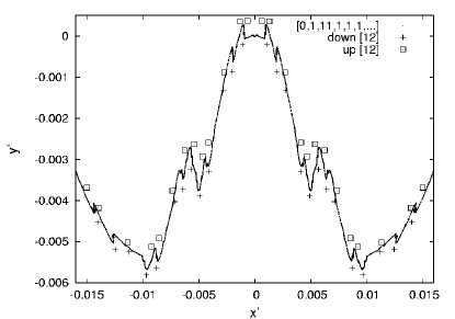
Figure 8: Two levels of magnification, in symmetry line coordinates ($x^{\prime},y^{\prime}$), of the $[0,1,11,1,1,1\ldots]$ meander at breakup. Also shown are the nearby up and down orbits of the $[12]$th (top) and $[24]$th (bottom) continued fraction convergents.

For a quantitative analysis, we compute the scaling factors $\alpha$ and $\beta$ such that the meander in the vicinity of its intersection with $s_{3}$ is invariant under $(x^{\prime},y^{\prime})\rightarrow(\alpha^{12}x^{\prime},\beta^{12}y^{\prime})$ (following the notation of Refs. Del-Castillo-Negrete et al., 1997; Apte et al., 2003). Again, these are found from the limiting behavior of convergent periodic orbits: Denoting by $(\hat{x}^{\prime}_{n,\pm},\hat{y}^{\prime}_{n,\pm})$ the symmetry line coordinates of the point on the up ($+$) or down ($-$) orbit of the $[n]$th convergent that is located closest to $(0,0)$, we compute

$$\alpha^{12}_{n,\pm}=\left|\frac{\hat{x}^{\prime}_{n,\pm}}{\hat{x}^{\prime}_{n+12,\pm}}\right|\>,\>\>\>\beta^{12}_{n,\pm}=\left|\frac{\hat{y}^{\prime}_{n,\pm}}{\hat{y}^{\prime}_{n+12,\pm}}\right|\>.$$ (9)

Averaging the six values $\alpha^{12}_{18\pm}$, $\alpha^{12}_{20\pm}$, and $\alpha^{12}_{22\pm}$, we find $\alpha^{12}=321.65\pm 0.070$, i.e., $\alpha=1.61789\pm 0.00003$ (with the error being the standard deviation of the mean). Similarly, for $\beta$, we obtain $\beta^{12}=431.29\pm 0.19$, i.e., $\beta=1.65792\pm 0.00006$. These are the scaling factors used in Fig. 8. Within numerical accuracy, they coincide with the values found in Refs. Del-Castillo-Negrete et al., 1997; Apte et al., 2003.

To interpret the scaling invariance of the shearless meander itself and its convergents under $[n]\rightarrow[n+12]$ one can introduce a renormalization picture, with a renormalization group operator ${\cal R}_{\omega}$ acting on the space of maps with shearless curve at winding number $\omega$ (see Refs. MacKay, 1983; Del-Castillo-Negrete et al., 1997; Apte et al., 2005). Operating with ${\cal R}_{[0,1,11,1,1,\ldots]}$ infinitely many times on the standard nontwist map at criticality of the shearless meander studied here limits to a map that is a period-12 fixed point, $\Lambda$, of the renormalization group operator.

In the vicinity of $\Lambda$, two unstable eigenvalues $\delta_{1}$ and $\delta_{2}$ can be computed to characterize the fixed point. As shown in Ref. Del-Castillo-Negrete et al., 1997, these are given by $\delta_{i}=\sqrt[12]{1/\nu_{i}}$, where

$$\nu_{1} = \lim_{n\rightarrow\infty}\left(\frac{b_{[n+12]}-b_{c}}{b_{[n]}-b_{c}}\right)\>,$$

$$\nu_{2} = \lim_{n\rightarrow\infty}\left(\frac{a_{c[n+12]}-a_{c}}{a_{c[n]}-a_{c}}\right)\>,$$ (10)

where $a_{c[n]}$ is the $a$-value along the bifurcation curve of the $[n]$th convergent, rather than along the shearless curve, at which the sequence of convergent residues exhibits nontrivial limiting behavior (i.e., converges neither to 0 nor $\infty$). Using $n=21$, we obtain the eigenvalues

$$\delta_{1}\approx 2.680\>,\>\>\>\delta_{2}\approx 1.584,$$ (11)

which are, within a small numerical error, the same values that were found for the $1/\gamma^{2}$ shearless curve in Ref. Apte et al., 2003, and, with a slightly larger error, for $1/\gamma$ in Ref. Del-Castillo-Negrete et al., 1997.

IV Breakup of the $\omega=[0,1,11,1,1,\ldots]$ outer shearless tori

IV.1 Search for critical parameter values

The procedure for finding the critical parameter values for the breakup of outer tori is the same as that described in Sec. III.1. The relations $y(b)$, at fixed $a$, for each of these orbits from Table 1 are found along symmetry lines. The collision parameters $b_{[n]}$ are again extrema of $b(y)$, only now the outer maxima are used, as illustrated in Fig. 9 for the lowest four convergents. The $b_{[n]}$ of the outer shearless orbits are marked by solid circles ($\bullet$). As in the central meander case, the best approximation to $b_{\infty}(a)$ (here $b_{[34]}$) is used for applying Greene’s residue criterion. Finally, varying $a$ to find the transition between residue convergence to 0 and $\infty$ results in the parameter values ($a_{co}$, $b_{co}$).

Figure 9: $y$-values in phase space of the 11/12, 12/13, 23/25, and 35/38 outer orbits on the $s_{1}$ symmetry line as a function of $b$, at $a=0.9757564461$.

Even though the $b_{[n]}(a)$ seem to follow the same scaling law, Eq. (3), as the ones approximating the central shearless meander, the data does not show sufficient evidence for a periodicity of $B(n)$. Using the numerical value for $\delta_{1}$ from Eq. (5) to allow for a direct comparison, and again plotting the offsets of the logarithmic $b_{[n]}$ differences about this average slope, Fig. 10 is obtained. Without an apparent periodicity, a better approximation to $b_{\infty}$ than $b_{[34]}$ , similar to the extrapolation in Eq. (6), cannot be found.

Figure 10: $b_{[n]}$ differences in approximating the critical shearless $\omega=[0,1,11,1,1,\ldots]$ outer orbits at $a_{co}=0.9757564461$ on the $s_{1}$ (above) and $s_{4}$ (below) symmetry lines.

IV.2 Residues at breakup

As before, we search along $\left(a,b_{[34]}(a)\right)$ for the transition between residue convergence to 0 and $\infty$. However, unlike before, where the critical parameters could be determined very accurately by observing significant deviations from the residue six-cycle for small changes in parameters, here the determination of the exact point of breakup is slightly less accurate. Because no clear cycle pattern is apparent, the only criterion to rely on is the residue convergence to 0 and $\infty$, which, however, leaves a transition range where the convergence of numerical data is inconclusive. With this in mind, our “best guess” for the critical parameters for the outer shearless tori breakup is:

$$(a_{co},b_{co})=(0.9757564461,0.1878717476259388)\;,$$ (12)

where the last digit in $a_{co}$ and several of the last digits in $b_{co}$ are merely conjectured to be the values that produce the “best transitional behavior” in the residue plots in Fig. 11. For a better view of the accuracy of these critical parameters, all parameters used are listed in Table 4.

Figure 11: Residue behavior for orbits on $s_{1}$ to $s_{4}$ at the breakup of $\omega=[0,1,11,1,1,\ldots]$ outer shearless tori. Residues for assumed breakup parameter values $(a_{co},b_{co})$ are indicated by the bold line. Residues for five parameter values with $a<a_{co}$ in steps of $10^{-10}$ are indicated by thin lines and residues for five parameter values with $a>a_{co}$ in steps of $10^{-10}$ by dotted lines.

$a_{[34]}$	$b_{[34]}$
0.9757564459	0.1878717467093720
0.9757564460	0.1878717471676554
0.9757564461	0.1878717476259388
0.9757564462	0.1878717480842221
0.9757564463	0.1878717485425054

Table 4: Numerical values of the critical parameters $(a_{[34]},b_{[34]})$ in the vicinity of the shearless outer tori breakup, with the conjectured critical parameters shown in italics.

In this case, the only (pairs of) existing periodic orbits $[n]$ of Table 1 are the ones with odd $n$. Since the outer shearless orbits (each considered separately) are not $S$-invariant, a residue correspondence scheme as in Table 2 does not exist. Therefore residues for both orbits on all four symmetry lines are shown in Fig. 11.

In contrast to all previous studies of breakups of central shearless tori with noble winding number, for the outer, non-$S$-invariant tori, no six-cycles occur. Whether the residues converge to higher period cycles remains an open question, since within the limited number of 19 data points that could be obtained numerically with sufficient accuracy (up to $[n]=[37]$ with only odd $[n]$ existing) no such cycle could be clearly identified, but certainly not ruled out either. What can be established, however, is that the outer shearless tori represent the first example where a breakup type different from a residue six-cycle is observed in the standard nontwist map.

IV.3 Phase space at breakup

The phase space at the critical parameter values for the breakup of the outer shearless tori is shown in Fig. 12. In contrast to the case of the central meander no scaling invariance was found.

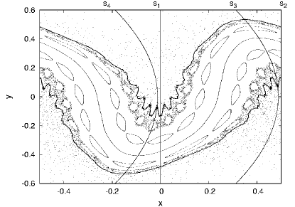
Figure 12: Phase space of the $[0,1,11,1,1,1\ldots]$ outer shearless tori at breakup, where $a_{co}=0.9757564461$ and $b_{co}=0.1878717476259388$. The symmetry lines $s_{1}$ to $s_{4}$ are shown.

V Regularity of critical invariant tori

The shearless irrational orbits can be described by a function called the “hull function.” For an invariant torus of rotation number $\omega$, this is given by the map $K:{\mathbb{T}}\to{\mathbb{T}}\times{\mathbb{R}}$ such that $M\circ K(\theta)=K(\theta+\omega),$ and the range of $K$ is the invariant torus under consideration. We choose the lift $\tilde{K}:{\mathbb{R}}\to{\mathbb{R}}\times{\mathbb{R}}$ of the map $K$ to satisfy

$$\tilde{K}(\theta+1)=\tilde{K}(\theta)+(1,0)\,,$$ (13)

which corresponds to the lift $\tilde{M}$ of the SNM satisfying $\tilde{M}(x+1,y)=\tilde{M}(x,y)+(1,0).$ Equation (13) also implies that the functions $\tilde{K}_{x}(\theta)-\theta$ and $\tilde{K}_{y}(\theta)$ are periodic. These functions for the critical central and outer meanders are shown in Fig. 13.

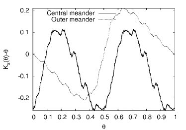
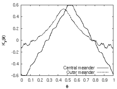
Figure 13: The hull functions $K_{x}(\theta)-\theta$ (left) and $K_{y}(\theta)$ (right) for the critical central and outer meanders.

We studied these functions using techniques from harmonic analysis developed in Refs. de la Llave and Petrov, 2002; Apte et al., 2004. In particular, Fig. 14 shows the plot of $\log\|(\partial/\partial t)^{\eta}e^{-t\sqrt{-d^{2}/d\theta^{2}}}K(\theta)\|_{L^{\infty}}$ versus $\log t$, calculated using $2^{25}$ Fourier coefficients of $K(\theta)$.

Figure 14: The plot of $\log\|(\partial/\partial t)^{\eta}e^{-t\sqrt{-d^{2}/d\theta^{2}}}K(\theta)\|_{L^{\infty}}$ versus $\log t$ for the hull functions.

We see that these functions saturate the bounds given in Ref. Stein, 1970, Ch. 5, Lemma 5: $\|(\partial/\partial t)^{\eta}e^{-t\sqrt{-d^{2}/d\theta^{2}}}K(\theta)\|_{L^{\infty}}\leq Ct^{\alpha-\eta}$, where $\alpha$ is the Holder exponent of $K$. This allows us to calculate the regularity of these hull functions from the slope of lines in Fig. 14 and the results are presented in Table 5. We conclude that the regularity of the central shearless torus is $0.68\pm 0.02$ while that of the outer torus is $0.72\pm 0.05$.

$\eta$	Central torus	Outer torus
2	$0.670\pm 0.002$	$0.691\pm 0.004$
3	$0.669\pm 0.004$	$0.683\pm 0.005$
4	$0.670\pm 0.004$	$0.685\pm 0.006$
5	$0.671\pm 0.004$	$0.665\pm 0.006$
$K_{x}(\theta)$	$0.67\pm 0.01$	$0.69\pm 0.01$
$\eta$	Central torus	Outer torus
2	$0.692\pm 0.003$	$0.756\pm 0.003$
3	$0.696\pm 0.003$	$0.757\pm 0.003$
4	$0.693\pm 0.003$	$0.769\pm 0.004$
5	$0.694\pm 0.004$	$0.757\pm 0.004$
$K_{y}(\theta)$	$0.69\pm 0.01$	$0.76\pm 0.01$

Table 5: The regularities of hull functions $K_{x}(\theta)-\theta$ (top) and $K_{y}(\theta)$(bottom), found using the slopes of lines in Fig. 14

This agrees very well with the regularity of other shearless noble tori studied in Ref. Apte et al., 2004.

VI Conclusion

In this paper we presented the breakup of two types of shearless invariant tori with noble winding number that had not been studied previously: a central meander and an outer torus. The breakup of the central meander showed within numerical accuracy the same critical residues, scaling parameters, and eigenvalues of the renormalization group operator as the central shearless invariant tori previously studied. From a renormalization group point of view this was to be expected: all nontwist maps with a critical shearless torus of noble winding number are expected to be equivalent under renormalization to the map with the critical shearless golden mean torus, independent of being a meander or not.

In this light, the result of the outer torus breakup is surprising. Although the winding number is noble, no critical residue pattern could be established within the numerically accessible range. This suggests that the number theoretic properties of the winding number might not be enough for the classification of different breakup scenarios. In the case of nontwist maps the symmetry properties of the shearless torus (here: $S$-invariant vs. not $S$-invariant) seem to affect the breakup. It is possible that after an appropriate coordinate change, that will make the outer torus symmetric in those coordinates, the SNM with critical outer torus is equivalent under renormalization to the fixed point with critical shearless golden mean torus. Alternatively, this could be the first indication of a new fixed point of the renormalization group operator for area-preserving maps.

Appendix A Basic definitions

For reference, we list a few basic definitions used throughout the main text:

An orbit of an area-preserving map $M$ is a sequence of points $\left\{\left(x_{i},y_{i}\right)\right\}_{i=-\infty}^{\infty}$ such that $M\left(x_{i},y_{i}\right)=\left(x_{i+1},y_{i+1}\right)$. The winding number $\omega$ of an orbit is defined as the limit $\omega=\lim_{i\to\infty}(x_{i}/i)$, when it exists. Here the $x$-coordinate is “lifted” from ${\mathbb{T}}$ to ${\mathbb{R}}$. A periodic orbit of period $n$ is an orbit $M^{n}\left(x_{i},y_{i}\right)=\left(x_{i}+m,y_{i}\right)$, $\forall\>i$, where $m$ is an integer. Periodic orbits have rational winding numbers $\omega=m/n$. An invariant torus is a one-dimensional set $C$, a curve, that is invariant under the map, $C=M(C)$. Of particular importance are the invariant tori that are homeomorphic to a circle and wind around the $x$-domain because, in two-dimensional maps, they act as transport barriers. Orbits belonging to such a torus generically have irrational winding number.

A map $M$ is called reversible if it can be decomposed as $M=I_{1}\circ I_{2}$ with $I_{i}^{2}=0$. The fixed point sets of $I_{i}$ are one-dimensional sets, called the symmetry lines of the map. For the SNM the symmetry lines are $s_{1}=\{(x,y)|x=0\}$, $s_{2}=\{(x,y)|x=1/2\}$, $s_{3}=\{(x,y)|x=a\left(1-y^{2}\right)/2\}$, and $s_{4}=\{(x,y)|x=a\left(1-y^{2}\right)/2+1/2\}$.

The $m/n$-bifurcation curve $b=\Phi_{m/n,i}(a)$ is the set of $(a,b)$ values for which the $m/n$ up and down periodic orbits on the symmetry line $s_{i}$ are at the point of collision. The main property of this curve is that for $(a,b)$ values below $b=\Phi_{m/n,i}(a)$, the $r/s$ periodic orbits with $r/s<m/n$ exist. Thus, $m/n$ is the maximum winding number for parameter values along the $m/n$ bifurcation curve. As detailed in Ref. Wurm et al., 2005, in certain parameter regions multiple orbits of winding number $m/n$, and therefore multiple bifurcation curves of the same winding number, can exist.

References

- Del-Castillo-Negrete and Morrison (1993) D. Del-Castillo-Negrete and P. J. Morrison, Phys. Fluids A 5, 948 (1993).
- Wurm et al. (2005) A. Wurm, A. Apte, K. Fuchss, and P. J. Morrison, Chaos 15, 023108 (2005).
- Apte et al. (2003) A. Apte, A. Wurm, and P. J. Morrison, Chaos 13, 421 (2003).
- Del-Castillo-Negrete et al. (1996) D. Del-Castillo-Negrete, J. M. Greene, and P. J. Morrison, Physica D 91, 1 (1996).
- Howard and Hohs (1984) J. E. Howard and S. M. Hohs, Phys. Rev. A 29, 418 (1984).
- Petrisor (2001) E. Petrisor, Int. J. of Bifur. and Chaos 11, 497 (2001).
- Apte et al. (2006) A. Apte, R. de la Llave, and E. Petrisor, Chaos Solit. and Fract. 27, 1115 (2006).
- Petrisor (2002) E. Petrisor, Chaos, Solit. and Fract. 14, 117 (2002).
- Wurm et al. (2004) A. Wurm, A. Apte, and P. J. Morrison, Brazilian J. of Phys 34, 1700 (2004).
- Shinohara and Aizawa (1997) S. Shinohara and Y. Aizawa, Progr. of Theor. Phys. 97, 379 (1997).
- Wurm (2002) A. Wurm, Ph.D. thesis, The University of Texas at Austin, Austin, Texas (2002).
- Apte et al. (2005) A. Apte, A. Wurm, and P. J. Morrison, Physica D 200, 47 (2005).
- Apte (2004) A. Apte, Ph.D. thesis, The University of Texas at Austin, Austin, Texas (2004).
- Greene (1979) J. M. Greene, J. Math. Phys. 20, 1183 (1979).
- Delshams and de la Llave (2000) A. Delshams and R. de la Llave, SIAM J. Math. Anal. 31, 1235 (2000).
- MacKay (1982) R. S. MacKay, Ph.D. dissertation, Princeton (1982), (also published by World Scientific, 1993).
- MacKay (1983) R. S. MacKay, Physica D 7, 283 (1983).
- Del-Castillo-Negrete et al. (1997) D. Del-Castillo-Negrete, J. M. Greene, and P. J. Morrison, Physica D 100, 311 (1997).
- de la Llave and Petrov (2002) R. de la Llave and N. P. Petrov, Experimental Math. 11, 219 (2002).
- Apte et al. (2004) A. Apte, R. de la Llave, and N. P. Petrov, Nonlinearity 18, 1173 (2004).
- Stein (1970) E. M. Stein, Singular Integrals and Differentiability Properties of Functions (Princeton University Press, Princeton, 1970).