Abstract

We study stability of interacting nonlinear systems with time-delayed communications, using contraction theory and a simplified wave variable design inspired by robotic teleoperation. We show that contraction is preserved through specific time-delayed feedback communications, and that this property is independent of the values of the delays. The approach is then applied to group cooperation with linear protocols, where it shown that synchronization can be made robust to arbitrary time delays.

1 Introduction

In many engineering applications, communications delays between subsystems cannot be neglected. Such an example is bilateral teleoperation, where signals can experience significant transmission delays between local and remote sites. Throughout the last decade, both internet and wireless technologies have vastly extended practical communication distances. Information exchange and cooperation can now occur in very widely distributed systems, making the effect of time delays even more central.

In the context of telerobotics, [2] proposed a control law for force-reflecting teleoperators which preserves passivity, and thus overcomes the instability caused by time delays. The idea was reformulated in [17] in terms of scattering or “wave” variables. Transmission of wave variables across communication channels ensures stability without knowledge of the time delay. Further extensions to internet-based applications were developed [15, 16, 3], in which communication delays are variable.

Recently, [13, 24] extended the application of wave variables to a more general context by performing a nonlinear contraction analysis [11, 13, 1, 5] of the effect of time-delayed communications between contracting systems. This paper modifies the design of the wave variables proposed in [13, 24]. Specifically, a simplified form provides an effective analysis tool for interacting nonlinear systems with time-delayed feedback communications. For appropriate coupling terms, contraction as a generalized stability property is preserved regardless of the delay values. The result also sheds a new light on the well-known fact in bilateral teleoperation, that even small time-delays in feedback PD controllers may create stability problems for simple coupled second-order systems, which motivated approaches based on passivity and wave variables [2, 17]. The approach is then applied to study the group cooperation problem with delayed communications. We show that synchronization with linear protocols [19, 14] is robust to time delays and network connectivity, without requiring the delays to be known or equal in all links. In a leaderless network, all the coupled elements tend to reach a common state which varies according to the initial conditions and the time delays, while in a leader-followers network the group agreement point is fixed by the leader. The approach is suitable to study both continuous and discrete-time models.

After brief reviews of nonlinear contraction and wave variables, Section $2$ uses simplified wave variable forms to analyze time-delayed feedback communications. The same approach is then applied in Section $3$ to study group cooperation. Concluding remarks are offered in Section $4$.

2 Contraction Analysis of Time-Delayed Communications

Inspired by the use of passivity [2] and wave variables [17] in force-reflecting teleoperation, [13] performed a contraction analysis of the effect of time-delayed communications. As we will discuss in this section, the form of the transmitted variables in [13] can be simplified and applied to analyze time-delayed feedback communications.

2.1 Background I: Contraction Theory

We first summarize briefly some basic definitions and main results of nonlinear contraction theory [11, 12]. Consider a nonlinear system

$$\dot{{\bf x}}={\bf f}({\bf x},t)$$ (1)

with ${\bf x}\in\mathbb{R}^{m\times 1}$ and ${\bf f}({\bf x},t)$ continuously differentiable. For any virtual displacement $\delta{\bf x}$ between two neighboring trajectories, we have

$$\frac{d}{dt}({\delta{\bf x}}^{T}{\delta{\bf x}})=2\ {\delta{\bf x}}^{T}{\delta\dot{{\bf x}}}=2\ {\delta{\bf x}}^{T}\frac{\partial{\bf f}}{\partial{\bf x}}\ {\delta{\bf x}}\leq 2\ \lambda_{max}\ {\delta{\bf x}}^{T}{\delta{\bf x}}$$

where $\lambda_{max}({\bf x},t)$ is the largest eigenvalue of the symmetric part of the Jacobian ${\bf J}=\frac{\partial{\bf f}}{\partial{\bf x}}$. Hence, if $\lambda_{max}({\bf x},t)$ is uniformly strictly negative, any infinitesimal length $\|\delta{\bf x}\|$ converges exponentially to zero. By path integration at fixed time, this implies that all the solutions converge exponentially to a single trajectory, independently of the initial conditions.

More generally, considering a coordinate transformation

$${\delta{\bf z}}={\bf\Theta}\delta{\bf x}$$ (2)

with square matrix ${\bf\Theta}({\bf x},t)$ uniformly invertible, we have

$$\frac{d}{dt}({\delta{\bf z}}^{T}{\delta{\bf z}})=2\ {\delta{\bf z}}^{T}{\delta\dot{\bf z}}=2\ {\delta{\bf z}}^{T}\ (\dot{{\bf\Theta}}+{\bf\Theta}\frac{\partial{\bf f}}{\partial{\bf x}}){\bf\Theta}^{-1}\ \delta{\bf z}$$

so that exponential convergence of $\|\delta{\bf z}\|$ to zero is guaranteed if the generalized Jacobian matrix

$${\bf F}=(\dot{\bf\Theta}+{\bf\Theta}\frac{\partial{\bf f}}{\partial{\bf x}}){\bf\Theta}^{-1}$$ (3)

is uniformly negative definite. Again, this implies in turn that all the solutions of the original system (1) converge exponentially to a single trajectory, independently of the initial conditions. Such a system is called contracting, with metric ${\bf\Theta}^{T}{\bf\Theta}$.

In the sequel, we will also use asymptotical contraction to refer to asymptotic convergence of any $\|\delta{\bf z}\|$ to zero, which implies global asymptotic convergence to a single trajectory.

2.2 Background II: Wave Variables

Wave variables [17] are used in bilateral teleoperation systems to guarantee the passivity [2] of time-delayed transmissions. The idea was generalized in [13] by conducting a contraction analysis on time-delayed transmission channels. As illustrated in Figure 1, [13] considers two interacting systems of possibly different dimensions,

$$\begin{cases}\ \dot{\bf x}_{1}\ =\ {\bf f}_{1}({\bf x}_{1},t)+{\bf G}_{21}{\bf\tau}_{21}\\ \ \dot{\bf x}_{2}\ =\ {\bf f}_{2}({\bf x}_{2},t)+{\bf G}_{12}{\bf\tau}_{12}\end{cases}$$ (4)

where ${\bf G}_{12}$, ${\bf G}_{21}$ are constant matrices and ${\bf\tau}_{12}$, ${\bf\tau}_{21}$ have the same dimension. Communication between the two systems occurs by transmitting intermediate “wave” variables, defined as

$${\bf u}_{21} = {\bf G}_{21}^{T}{\bf x}_{1}\ +\ {\bf\tau}_{21}\ \ \ \ \ \ \ \ \ \ \ \ \ \ \ \ \ {\bf v}_{12}={\bf G}_{21}^{T}{\bf x}_{1}\ -\ {\bf\tau}_{21}$$

$${\bf u}_{12} = {\bf G}_{12}^{T}{\bf x}_{2}\ +\ {\bf\tau}_{12}\ \ \ \ \ \ \ \ \ \ \ \ \ \ \ \ \ {\bf v}_{21}={\bf G}_{12}^{T}{\bf x}_{2}\ -\ {\bf\tau}_{12}$$

Because of time-delays, one has

$${\bf u}_{12}(t)={\bf v}_{12}(t-T_{12})\ \ \ \ \ \ \ \ \ \ \ \ \ \ \ \ {\bf u}_{21}(t)={\bf v}_{21}(t-T_{21})$$

where $T_{12}$ and $T_{21}$ are two positive constants. It can be proved that, if both ${\bf f}_{1}$ and ${\bf f}_{2}$ are contracting, the overall system is asymptotically contracting independently of the time delays.

Figure 1: Two interacting systems with delayed communications

Note that subscripts containing two numbers indicate the communication direction, e.g., subscript “$12$” refers to communication from node $1$ to $2$. This notation will be helpful in Section 3, where results will be extended to groups of interacting subsystems.

2.3 Time-Delayed Feedback Communications

Let us now consider modified choices of the transmitted variables above. Specifically, for interacting systems (4), define now the transmitted variables as

$${\bf u}_{21} = {\bf G}_{21}^{T}{\bf x}_{1}\ +\ k_{21}{\bf\tau}_{21}\ \ \ \ \ \ \ \ \ \ \ \ \ \ \ \ \ {\bf v}_{12}={\bf G}_{21}^{T}{\bf x}_{1}$$ (5)

$${\bf u}_{12} = {\bf G}_{12}^{T}{\bf x}_{2}\ +\ k_{12}{\bf\tau}_{12}\ \ \ \ \ \ \ \ \ \ \ \ \ \ \ \ \ {\bf v}_{21}={\bf G}_{12}^{T}{\bf x}_{2}$$

where $k_{12}$ and $k_{21}$ are two strictly positive constants. Consider, similarly to [13, 24], the differential length

$$V\ =\ \frac{k_{21}}{2}\ \delta{\bf x}_{1}^{T}\delta{\bf x}_{1}\ +\ \frac{k_{12}}{2}\ \delta{\bf x}_{2}^{T}\delta{\bf x}_{2}\ +\ \frac{1}{2}\ V_{1,2}$$

where

$$V_{1,2}=\int_{t-T_{12}}^{t}\delta{\bf v}_{12}^{T}\delta{\bf v}_{12}\ d\epsilon\ +\ \int_{t-T_{21}}^{t}\delta{\bf v}_{21}^{T}\delta{\bf v}_{21}\ d\epsilon\\ \ -\ \int_{-T_{12}}^{0}\delta{\bf v}_{12}^{T}\delta{\bf v}_{12}\ d\epsilon\ -\ \int_{-T_{21}}^{0}\delta{\bf v}_{21}^{T}\delta{\bf v}_{21}\ d\epsilon$$

Note that

$$V_{1,2} = \int_{0}^{t}(\ \delta{\bf v}_{12}^{T}\delta{\bf v}_{12}(\epsilon)-\delta{\bf v}_{12}^{T}\delta{\bf v}_{12}(\epsilon-T_{12})+\delta{\bf v}_{21}^{T}\delta{\bf v}_{21}(\epsilon)-\delta{\bf v}_{21}^{T}\delta{\bf v}_{21}(\epsilon-T_{21})\ )\ d\epsilon$$

$$= \int_{0}^{t}(\ \delta{\bf v}_{12}^{T}\delta{\bf v}_{12}(\epsilon)\ -\ \delta{\bf u}_{12}^{T}\delta{\bf u}_{12}(\epsilon)\ +\ \delta{\bf v}_{21}^{T}\delta{\bf v}_{21}(\epsilon)\ -\ \delta{\bf u}_{21}^{T}\delta{\bf u}_{21}(\epsilon)\ )\ d\epsilon$$

$$= -2\int_{0}^{t}(\ k_{21}\delta{\bf x}_{1}^{T}{\bf G}_{21}\delta{\bf\tau}_{21}+k_{12}\delta{\bf x}_{2}^{T}{\bf G}_{12}\delta{\bf\tau}_{12})\ d\epsilon\ -\int_{0}^{t}(\ k_{21}^{2}\delta{\bf\tau}_{21}^{T}\delta{\bf\tau}_{21}+k_{12}^{2}\delta{\bf\tau}_{12}^{T}\delta{\bf\tau}_{12})\ d\epsilon$$

This yields

$$\dot{V}\ =\ k_{21}\delta{\bf x}_{1}^{T}\frac{\partial{\bf f}_{1}}{\partial{\bf x}_{1}}\ \delta{\bf x}_{1}\ +\ k_{12}\delta{\bf x}_{2}^{T}\frac{\partial{\bf f}_{2}}{\partial{\bf x}_{2}}\ \delta{\bf x}_{2}\ -\ \frac{k_{21}^{2}}{2}\ \delta{\bf\tau}_{21}^{T}\delta{\bf\tau}_{21}\ -\ \frac{k_{12}^{2}}{2}\ \delta{\bf\tau}_{12}^{T}\delta{\bf\tau}_{12}$$

If ${\bf f}_{1}$ and ${\bf f}_{2}$ are both contracting with identity metrics (i.e., if $\frac{\partial{\bf f}_{1}}{\partial{\bf x}_{1}}$ and $\frac{\partial{\bf f}_{2}}{\partial{\bf x}_{2}}$ are both uniformly negative definite), then $\ \dot{V}\leq 0$, and $V$ is bounded and tends to a limit. Applying Barbalat’s lemma [23] in turn shows that, if $\ddot{V}$ is bounded, then $\dot{V}$ tends to zero asymptotically, which implies that $\delta{\bf x}_{1}$, $\delta{\bf x}_{2}$, $\delta{\bf\tau}_{12}$ and $\delta{\bf\tau}_{21}$ all tend to zero. Regardless of the values of the delays, all solutions of system (4) converge to a single trajectory, independently of the initial conditions. In the sequel we shall assume that $\ddot{V}$ can indeed be bounded as a consequence of the boundedness of $V$.

This result has a useful interpretation. Expanding system dynamics (4) using (5) yields

$$\begin{cases}\ \dot{\bf x}_{1}\ =\ {\bf f}_{1}({\bf x}_{1},t)\ +\ \frac{1}{k_{21}}\ {\bf G}_{21}\ (\ {\bf G}_{12}^{T}{\bf x}_{2}(t-T_{21})-{\bf G}_{21}^{T}{\bf x}_{1}(t)\ )\\ \ \dot{\bf x}_{2}\ =\ {\bf f}_{2}({\bf x}_{2},t)\ +\ \frac{1}{k_{12}}\ {\bf G}_{12}\ (\ {\bf G}_{21}^{T}{\bf x}_{1}(t-T_{12})-{\bf G}_{12}^{T}{\bf x}_{2}(t)\ )\end{cases}$$

so that the above communications in fact correspond to simple feedback interactions. If we assume further that ${\bf x}_{1}$ and ${\bf x}_{2}$ have the same dimension, and choose ${\bf G}_{12}={\bf G}_{21}={\bf G}$, the whole system is actually equivalent to two diffusively coupled subsystems

$$\begin{cases}\ \dot{\bf x}_{1}\ =\ {\bf f}_{1}({\bf x}_{1},t)\ +\ \frac{1}{k_{21}}\ {\bf G}{\bf G}^{T}\ (\ {\bf x}_{2}(t-T_{21})-{\bf x}_{1}(t)\ )\\ \ \dot{\bf x}_{2}\ =\ {\bf f}_{2}({\bf x}_{2},t)\ +\ \frac{1}{k_{12}}\ {\bf G}{\bf G}^{T}\ (\ {\bf x}_{1}(t-T_{12})-{\bf x}_{2}(t)\ )\end{cases}$$ (6)

Note that constants $k_{12}$ and $k_{21}$ and thus coupling gains along different diffusion directions can be different. We can thus state

Theorem 1

Consider two subsystems, both contracting with identity metrics, and interacting through time-delayed diffusion-like couplings (6). Then the overall system is asymptotically contracting.

Figure 2: Two interacting systems with time-delayed diffusion couplings

Remarks

• Theorem 1 does not contradict the well-known fact in teleoperation, that even small time-delays in bilateral PD controllers may create stability problems for coupled second-order systems [2, 17, 16, 3], which motivates approaches based on passivity and wave variables. In fact, a key condition for contraction to be preserved is that the diffusion-like coupling gains be symmetric positive semi-definite in the same metric as the subsystems, as we shall illustrate later in this section.

• If there are no delays, i.e., $T_{12}=T_{21}=0$, then $V_{1,2}=0$. Thus, the analysis of the differential length yields that

  $$\dot{V} = \frac{1}{2}\frac{d}{dt}(\ k_{21}\delta{\bf x}_{1}^{T}\delta{\bf x}_{1}\ +\ k_{12}\delta{\bf x}_{2}^{T}\delta{\bf x}_{2}\ )\ \leq\ k_{21}\delta{\bf x}_{1}^{T}\frac{\partial{\bf f}_{1}}{\partial{\bf x}_{1}}\delta{\bf x}_{1}\ +\ k_{12}\delta{\bf x}_{2}^{T}\frac{\partial{\bf f}_{2}}{\partial{\bf x}_{2}}\delta{\bf x}_{2}$$

  $$\leq \lambda_{max}\ (\ k_{21}\delta{\bf x}_{1}^{T}\delta{\bf x}_{1}\ +\ k_{12}\delta{\bf x}_{2}^{T}\delta{\bf x}_{2}\ )$$

  where

  $$\lambda_{max}\ =\ \max(\ \lambda_{max}(\frac{\partial{\bf f}_{1}}{\partial{\bf x}_{1}})_{s},\ \lambda_{max}(\frac{\partial{\bf f}_{2}}{\partial{\bf x}_{2}})_{s}\ )$$

  This implies that $\delta{\bf x}_{1}$ and $\delta{\bf x}_{2}$ tend to zero exponentially for contracting dynamics ${\bf f}_{1}$ and ${\bf f}_{2}$, i.e., the overall system is exponentially contracting.

• If ${\bf f}_{1}$ and ${\bf f}_{2}$ are both contracting and time-invariant, all solutions of system (6) converge to a unique equilibrium point, whose value is independent of the time delays and the initial conditions. Indeed, in a globally contracting autonomous system, all trajectories converge to a unique equilibrium point [11, 22], which implies that if ${\bf f}_{1}$ and ${\bf f}_{2}$ are both contracting and time-invariant, an equilibrium point must exist for system (6) when $T_{12}=T_{21}=0$. In turn, this point remains an equilibrium point for arbitrary non-zero $T_{12}$ and $T_{21}$. Since the delayed system (6) also preserves contraction, all solutions will converge to this point independently of the initial conditions and the explicit values of the delays.

• Theorem 1 can be extended directly to study more general connections between groups, such as bidirectional meshes or webs of arbitrary size, and parallel unidirectional rings of arbitrary length, both of which will be illustrated through Section 3. Inputs to the overall system can be provided through any of the subgroup dynamics.

• Example 2.1

  : Consider two identical second-order systems coupled through time-delayed feedback PD controllers

  $$\begin{cases}\ \ddot{x}_{1}+b\dot{x}_{1}+\omega^{2}x_{1}\ =\ k_{d}(\dot{x}_{2}(t-T_{21})-\dot{x}_{1}(t))+k_{p}(x_{2}(t-T_{21})-x_{1}(t))\\ \ \ddot{x}_{2}+b\dot{x}_{2}+\omega^{2}x_{2}\ =\ k_{d}(\dot{x}_{1}(t-T_{12})-\dot{x}_{2}(t))+k_{p}(x_{1}(t-T_{12})-x_{2}(t))\end{cases}$$

  with $b>0$, $\omega>0$. If $T_{12}=T_{21}=0$, partial contraction analysis [25, 31] shows that $x_{1}$ and $x_{2}$ converge together exponentially regardless of initial conditions, which makes the origin a stable equilibrium point. If $T_{12},T_{21}>0$, a simple coordinate transformation yields

  $$\left[\begin{array}[]{l}\dot{x}_{1}\\ \dot{y}_{1}\end{array}\right] = \left[\begin{array}[]{c}\omega y_{1}-bx_{1}\\ -\omega x_{1}\end{array}\right]+{\bf K}(\left[\begin{array}[]{l}x_{2}(t-T_{21})\\ y_{2}(t-T_{21})\end{array}\right]-\left[\begin{array}[]{l}x_{1}(t)\\ y_{1}(t)\end{array}\right])$$

  $$\left[\begin{array}[]{l}\dot{x}_{2}\\ \dot{y}_{2}\end{array}\right] = \left[\begin{array}[]{c}\omega y_{2}-bx_{2}\\ -\omega x_{2}\end{array}\right]+{\bf K}(\left[\begin{array}[]{l}x_{1}(t-T_{12})\\ y_{1}(t-T_{12})\end{array}\right]-\left[\begin{array}[]{l}x_{2}(t)\\ y_{2}(t)\end{array}\right])$$

  where

  $${\bf f}_{1}=\left[\begin{array}[]{c}\omega y_{1}-bx_{1}\\ -\omega x_{1}\end{array}\right]\ \ \ \ \ \ \ \ \rm{and}\ \ \ \ \ \ \ {\bf f}_{2}=\left[\begin{array}[]{c}\omega y_{2}-bx_{2}\\ -\omega x_{2}\end{array}\right]$$

  are both contracting with identity metric [31]. However, the transformed coupling gain

  $${\bf K}=\left[\begin{array}[]{ll}k_{d}&0\\ \frac{k_{p}}{\omega}&0\end{array}\right]$$

  is neither symmetric nor positive semi-definite for any $k_{p}\neq 0$. Contraction cannot be preserved in this case, and the coupled systems turn out to be unstable for large enough delays as the simulation result in Figure 3(a) illustrates. In Figure 3(b) we set $k_{p}=0$ so that the overall system is contracting according to Theorem 1. $\Box$

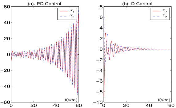
Figure 3: Simulation results of two coupled mass-spring-damper systems with (a) PD control and (b) D control. Parameters are $b=0.5$, $\omega^{2}=5$, $T_{12}=2s$, $T_{21}=4s$, $k_{d}=1,$ $k_{p}=5$ in (a) and $k_{p}=0$ in (b). Initial conditions, chosen randomly, are identical for the two plots.

The instability mechanism in the above example is actually very similar to that of the classical Smale model [27, 31] of spontaneous oscillation, in which two or more identical biological cells, inert by themselves, tend to self-excited oscillations through diffusion interactions. In both cases, the instability is caused by a non-identity metric, which makes the transformed coupling gains lose positive semi-definiteness. Note that the relative simplicity with which both phenomena can be analyzed makes fundamental use of the notion of a metric, central to contraction theory.

2.4 Other Simplified Forms of Wave-Variables

Different simplifications of the original wave-variable design can be made based on the same choice of $V$, yielding different qualitative properties. For instance, the transmitted signals can be defined as

$${\bf u}_{21} = {\bf G}_{21}^{T}{\bf x}_{1}\ +\ k_{21}{\bf\tau}_{21}\ \ \ \ \ \ \ \ \ \ \ \ \ \ \ \ {\bf v}_{12}=-\ k_{21}{\bf\tau}_{21}$$

$${\bf u}_{12} = {\bf G}_{12}^{T}{\bf x}_{2}\ +\ k_{12}{\bf\tau}_{12}\ \ \ \ \ \ \ \ \ \ \ \ \ \ \ \ {\bf v}_{21}=-\ k_{12}{\bf\tau}_{12}$$

which leads to

$$\dot{V} = k_{21}\delta{\bf x}_{1}^{T}\frac{\partial{\bf f}_{1}}{\partial{\bf x}_{1}}\delta{\bf x}_{1}\ +\ k_{12}\delta{\bf x}_{2}^{T}\frac{\partial{\bf f}_{2}}{\partial{\bf x}_{2}}\delta{\bf x}_{2}\ -\ \frac{1}{2}\delta{\bf x}_{1}^{T}{\bf G}_{21}{\bf G}_{21}^{T}\delta{\bf x}_{1}\ -\ \frac{1}{2}\delta{\bf x}_{2}^{T}{\bf G}_{12}{\bf G}_{12}^{T}\delta{\bf x}_{2}$$ (9)

$$= \delta{\bf x}_{1}^{T}(\ k_{21}\frac{\partial{\bf f}_{1}}{\partial{\bf x}_{1}}\ -\frac{1}{2}{\bf G}_{21}{\bf G}_{21}^{T}\ )\delta{\bf x}_{1}\ +\ \delta{\bf x}_{2}^{T}(\ k_{12}\frac{\partial{\bf f}_{2}}{\partial{\bf x}_{2}}\ -\frac{1}{2}{\bf G}_{12}{\bf G}_{12}^{T}\ )\delta{\bf x}_{2}$$

and thus also preserves contraction through time-delayed communications. Similarly to the previous section, if both ${\bf f}_{1}$ and ${\bf f}_{2}$ are contracting and time-invariant, the whole system tends towards a unique equilibrium point, regardless of the delay values. At this steady state, ${\bf u}_{12}(\infty)\ =\ {\bf v}_{12}(\infty)$ and ${\bf u}_{21}(\infty)\ =\ {\bf v}_{21}(\infty)$, which immediately implies that

$${\bf G}_{21}^{T}\ {\bf x}_{1}(\infty)\ =\ {\bf G}_{12}^{T}\ {\bf x}_{2}(\infty)$$

and, if ${\bf G}_{12}={\bf G}_{21}={\bf G}$ with ${\bf G}$ of full rank, that

$${\bf x}_{1}(\infty)\ =\ {\bf x}_{2}(\infty)$$

Thus, contrary to the case (5) of diffusion-like couplings, the remote tracking ability of wave variables is preserved.

• Example 2.2

  : Consider the example of two second-order systems

  $$\begin{cases}\ \ddot{x}_{1}+b_{1}\dot{x}_{1}+\omega_{1}^{2}x_{1}\ =\ F_{21}\ +\ F_{e}\\ \ \ddot{x}_{2}+b_{2}\dot{x}_{2}+\omega_{2}^{2}x_{2}\ =\ F_{12}\end{cases}$$

  where $F_{e}$ is an external force, and $F_{21}$, $F_{12}$ are internal forces undergoing time delays. Performing a coordinate transformation, we get new equations

  $$\left[\begin{array}[]{l}\dot{x}_{1}\\ \dot{y}_{1}\end{array}\right] = \left[\begin{array}[]{c}\omega_{1}y_{1}-b_{1}x_{1}\\ -\omega_{1}x_{1}+\frac{F_{e}}{\omega_{1}}\end{array}\right]\ +\ \left[\begin{array}[]{l}0\\ \frac{F_{21}}{\omega_{1}}\end{array}\right]$$

  $$\left[\begin{array}[]{l}\dot{x}_{2}\\ \dot{y}_{2}\end{array}\right] = \left[\begin{array}[]{c}\omega_{2}y_{2}-b_{2}x_{2}\\ -\omega_{2}x_{2}\end{array}\right]\ +\ \left[\begin{array}[]{l}0\\ \frac{F_{12}}{\omega_{2}}\end{array}\right]$$

  The signals being transmitted are defined as simplified wave variables

  $$u_{21} = y_{1}\ +\ \frac{k_{21}}{\omega_{1}}F_{21}\ \ \ \ \ \ \ \ \ \ \ \ \ \ \ \ v_{12}=-\ \frac{k_{21}}{\omega_{1}}F_{21}$$

  $$u_{12} = y_{2}\ +\ \frac{k_{12}}{\omega_{2}}F_{12}\ \ \ \ \ \ \ \ \ \ \ \ \ \ \ \ v_{21}=-\ \frac{k_{12}}{\omega_{2}}F_{12}$$

  Note that here ${\bf G}_{12}={\bf G}_{21}=\left[\begin{array}[]{cc}0&0\\ 0&1\end{array}\right]$, and that although the variables $y_{1}$ and $y_{2}$ are virtual, their values can be calculated based on $x_{1}$, $\dot{x}_{1}$ and $x_{2}$, $\dot{x}_{2}$. According to the result we derived above, the whole system will tend to reach an equilibrium point asymptotically. This point is independent to the time delays and satisfies $y_{1}(\infty)\ =\ y_{2}(\infty)$, i.e.,

  $$\frac{b_{1}}{\omega_{1}}x_{1}(\infty)\ =\ \frac{b_{2}}{\omega_{2}}x_{2}(\infty)$$

  $\Box$

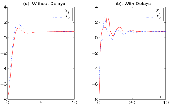
Figure 4: Simulation results of Example 2.2 with (a). $T_{12}=T_{21}=0$ and with (b). $T_{12}=2s$, $T_{21}=4s$. The parameters are $b_{1}=b_{2}=0.5$, $\omega_{1}^{2}=\omega_{2}^{2}=5$, $k_{12}=k_{21}=0.2$, and $F_{e}=10$. Initial conditions, chosen randomly, are identical for the two plots. Convergence to a common equilibrium point independent to the time delays is achieved in both cases.

Finally note that even if the subsystems are not contracting but have upper bounded Jacobian, for instance, as limit-cycle oscillators, the overall system still can be contracting by choosing appropriate gains such that

$${\bf G}_{21}{\bf G}_{21}^{T}\ >\ 2k_{21}(\frac{\partial{\bf f}_{1}}{\partial{\bf x}_{1}})_{s}\ \ \ \ \ \ \ \ \ \rm{and}\ \ \ \ \ \ \ \ \ \ {\bf G}_{12}{\bf G}_{12}^{T}\ >\ 2k_{12}(\frac{\partial{\bf f}_{2}}{\partial{\bf x}_{2}})_{s}$$

Here the transmission of wave variables performs a stabilizing role.

There are also other simplified forms of wave variables. For instance, we can define the transmitted signals as

$${\bf u}_{21} = {\bf G}_{21}^{T}{\bf x}_{1}\ +\ k_{21}{\bf\tau}_{21}\ \ \ \ \ \ \ \ \ \ \ \ \ \ \ \ \ {\bf v}_{12}=k_{21}{\bf\tau}_{21}$$

$${\bf u}_{12} = {\bf G}_{12}^{T}{\bf x}_{2}\ +\ k_{12}{\bf\tau}_{12}\ \ \ \ \ \ \ \ \ \ \ \ \ \ \ \ \ {\bf v}_{21}=k_{12}{\bf\tau}_{12}$$

If both ${\bf f}_{1}$ and ${\bf f}_{2}$ are contracting and time-invariant, and if ${\bf G}_{12}={\bf G}_{21}={\bf G}$ with ${\bf G}$ of full rank, the whole system tends towards a unique equilibrium point such that $\ {\bf x}_{1}(\infty)\ =\ -\ {\bf x}_{2}(\infty)$.

3 Group Cooperation with Time-Delayed Communications

Recently, synchronization or group agreement has been the object of extensive literature [6, 9, 10, 18, 20, 21, 22, 28, 29, 30]. Understanding natural aggregate motions as in bird flocks, fish schools, or animal herds may help achieve desired collective behaviors in artificial multi-agent systems. In our previous work [25, 31], a synchronization condition was obtained for a group of coupled nonlinear systems, where the number of the elements can be arbitrary and the network structure can be very general. In this section, we study a simplified continuous-time model of schooling or flocking with time-delayed communications, and generalize recent results in the literature [19, 14]. In particular, we show that synchronization is robust to time delays both for the leaderless case and for the leader-followers case, without requiring the delays to be known or equal in all links. Similar results are then derived for discrete-time models.

3.1 Leaderless Group

We first investigate a flocking model without group leader. The dynamics of the $i$th element is given as

$$\dot{\bf x}_{i}\ =\ \sum_{j\in{\mathcal{N}}_{i}}{\bf K}_{ji}\ ({\bf x}_{j}-{\bf x}_{i})\ \ \ \ \ \ \ \ \ \ \ \ \ \ \ \ \ \ \ \ \ i=1,\ldots,n$$ (12)

where $\ {\bf x}_{i}\in\mathbb{R}^{m}\$ denotes the states needed to reach agreements such as a vehicle’s heading, attitude, velocity, etc. $\ {\mathcal{N}}_{i}\$ denotes the set of the active neighbors of element $i$, which for instance can be defined as the set of the nearest neighbors within a certain distance around $i$. $\ {\bf K}_{ji}\$ is the coupling gain, which is assumed to be symmetric and positive definite.

Theorem 2

Consider $n$ coupled elements with linear protocol (12). The whole system will tend to reach a group agreement

$${\bf x}_{1}(t)=\cdots={\bf x}_{n}(t)=\frac{1}{n}({\bf x}_{1}(0)+\cdots+{\bf x}_{n}(0))$$

exponentially if the network is connected, and the coupling links are either bidirectional with ${\bf K}_{ji}={\bf K}_{ij}$, or unidirectional but formed in closed rings with identical gains.

Theorem 2 is derived in [25, 31] based on partial contraction analysis, and the result can be extended further to time-varying couplings (${\bf K}_{ji}={\bf K}_{ji}(t)$), switching networks (${\mathcal{N}}_{i}={\mathcal{N}}_{i}(t)$) and looser connectivity conditions.

Assume now that time delays are non-negligible in communications. The dynamics of the $i$th element then turns to be

$$\dot{\bf x}_{i}\ =\ \sum_{j\in{\mathcal{N}}_{i}}{\bf K}_{ji}\ (\ {\bf x}_{j}(t-T_{ji})-{\bf x}_{i}(t)\ )$$ (13)

Theorem 3

Consider $n$ coupled elements (13) with time-delayed communications. Regardless of the explicit values of the delays, the whole system will tend to reach a group agreement ${\bf x}_{1}(t)=\cdots={\bf x}_{n}(t)$ asymptotically if the network is connected, and the coupling links are either bidirectional with ${\bf K}_{ji}={\bf K}_{ij}$, or unidirectional but formed in closed rings with identical gains.

Proof:   For notational simplicity, we first assume that all the links are bidirectional with ${\bf K}_{ji}={\bf K}_{ij}$, but the time delays could be different along the opposite directions, i.e., $T_{ji}\neq T_{ij}$. Thus, Equation (13) can be transformed to

$$\dot{\bf x}_{i}\ =\ \sum_{j\in{\mathcal{N}}_{i}}{\bf G}_{ji}{\bf\tau}_{ji}$$

where ${\bf\tau}_{ji}$ and correspondingly ${\bf\tau}_{ij}$ are defined as

$${\bf u}_{ji} = {\bf G}_{ji}^{T}{\bf x}_{i}\ +\ {\bf\tau}_{ji}\ \ \ \ \ \ \ \ \ \ \ \ \ \ \ {\bf v}_{ij}={\bf G}_{ji}^{T}{\bf x}_{i}$$ (14)

$${\bf u}_{ij} = {\bf G}_{ij}^{T}{\bf x}_{j}\ +\ {\bf\tau}_{ij}\ \ \ \ \ \ \ \ \ \ \ \ \ \ \ {\bf v}_{ji}={\bf G}_{ij}^{T}{\bf x}_{j}$$

with $\ {\bf G}_{ij}={\bf G}_{ji}>0\$ and $\ {\bf K}_{ji}={\bf K}_{ij}={\bf G}_{ij}{\bf G}_{ij}^{T}\$. Define

$$V\ =\ \frac{1}{2}\sum_{i=1}^{n}\delta{\bf x}_{i}^{T}\delta{\bf x}_{i}\ +\ \frac{1}{2}\sum_{(i,j)\in{\mathcal{N}}}\ V_{i,j}$$ (15)

where ${\mathcal{N}}=\cup_{i=1}^{n}{\mathcal{N}}_{i}$ denotes the set of all active links, and $V_{i,j}$ is defined as in Section 2.3 for each link connecting two nodes $i$ and $j$. Therefore

$$\dot{V}\ =\ -\frac{1}{2}\sum_{(i,j)\in{\mathcal{N}}}(\delta{\bf\tau}_{ji}^{T}\delta{\bf\tau}_{ji}+\delta{\bf\tau}_{ij}^{T}\delta{\bf\tau}_{ij})$$

One easily shows that $\ddot{V}$ is bounded. Thus according to Barbalat’s lemma, $\dot{V}$ will tend to zero asymptotically, which implies that, $\forall(i,j)\in{\mathcal{N}}$, $\delta{\bf\tau}_{ji}$ and $\delta{\bf\tau}_{ij}$ tend to zero asymptotically. Thus, we know that $\forall i$, $\delta\dot{\bf x}_{i}$ tends to zero. In standard calculus, a vanishing $\delta\dot{\bf x}_{i}$ does not necessarily mean that $\delta{\bf x}_{i}$ is convergent. But it does in this case because otherwise it will conflict with the fact that $\delta{\bf x}_{i}$ tends to be periodic with a constant period $T_{ji}+T_{ij}$, which can be shown since

$$\delta{\bf u}_{ji}(t) = {\bf G}_{ji}^{T}\delta{\bf x}_{i}(t)+\delta{\bf\tau}_{ji}(t)\ =\ {\bf G}_{ij}^{T}\delta{\bf x}_{j}(t-T_{ji})$$ (16)

$$\delta{\bf u}_{ij}(t) = {\bf G}_{ij}^{T}\delta{\bf x}_{j}(t)+\delta{\bf\tau}_{ij}(t)\ =\ {\bf G}_{ji}^{T}\delta{\bf x}_{i}(t-T_{ij})$$

From (16) we can also conclude that, if $\forall i\ \delta{\bf x}_{i}$ is convergent, they will tend to a steady state

$$\delta{\bf x}_{1}(t)=\cdots=\delta{\bf x}_{n}(t)={\bf c}$$

where ${\bf c}$ is a constant vector whose value dependents on the specific trajectories we analyze. Moreover, we notice that, in the state-space, any point inside the region ${\bf x}_{1}=\cdots={\bf x}_{n}$ is invariant to (13). By path integration, this implies immediately that, regardless of the delay values or the initial conditions, all solutions of the system (13) will tend to reach a group agreement ${\bf x}_{1}=\cdots={\bf x}_{n}$ asymptotically.

In case that coupling links are unidirectional but formed in closed rings with coupling gains identical in each ring, we set

$$V = \frac{1}{2}\sum_{i=1}^{n}\delta{\bf x}_{i}^{T}\delta{\bf x}_{i}\ +\ \frac{1}{2}\sum_{(j\to i)\in{\mathcal{N}}}\ (\ \int_{t-T_{ji}}^{t}\delta{\bf v}_{ji}^{T}\delta{\bf v}_{ji}d\epsilon-\int_{-T_{ji}}^{0}\delta{\bf v}_{ji}^{T}\delta{\bf v}_{ji}\ d\epsilon\ )$$

$$= \frac{1}{2}\sum_{i=1}^{n}\delta{\bf x}_{i}^{T}\delta{\bf x}_{i}\ +\ \frac{1}{2}\sum_{(j\to i)\in{\mathcal{N}}}\ \int_{0}^{t}(\ \delta{\bf v}_{ji}^{T}\delta{\bf v}_{ji}(\epsilon)-\delta{\bf v}_{ji}^{T}\delta{\bf v}_{ji}(\epsilon-T_{ji})\ )\ d\epsilon$$

and the rest of the proof is the same. The case when both types of links are involved is similar. $\Box$

• Example 3.1

  : Compared to Theorem 2, the group agreement point in Theorem 3 generally does not equal the average value of the initial conditions, but depends on the values of the time delays.

  Consider the cooperative group (13) with one-dimensional ${\bf x}_{i}$, $n=6$, and a two-way chain structure

  The coupling gains are set to be identical with value $k=5$. The delay values are different, and each is chosen randomly around $0.5$ second. Simulation results are plotted in Figure 5. $\Box$

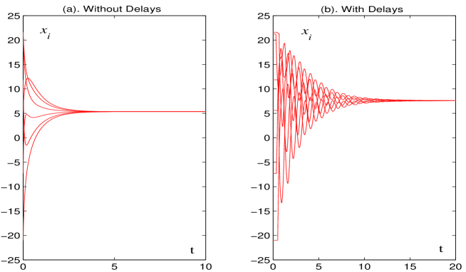
Figure 5: Simulation results of Example 3.1 without delays and with delays. Initial conditions, chosen randomly, are the same for each simulation. Group agreement is reached in both cases, although the agreement value is different.

Remarks

• The conditions on coupling gains can be relaxed. For instance, if the links are bidirectional, we do not have to ask ${\bf K}_{ij}={\bf K}_{ji}$. Instead, the dynamics of the $i$th element could be

  $$\dot{\bf x}_{i}\ =\ {\bf K}_{i}\ \sum_{j\in{\mathcal{N}}_{i}}\ (\ {\bf x}_{j}(t-T_{ji})-{\bf x}_{i}(t)\ )$$

  where ${\bf K}_{i}=\frac{1}{k_{i}}{\bf G}{\bf G}^{T}$ and ${\bf G}$ is unique through the whole network. The proof is the same except that we incorporate $k_{i}$ into the wave variables and the function $V$. Such a design brings more flexibility to cooperation-law design. The discrete-time model studied in Section 3.3 in in this spirit. A similar condition was derived in [4] for a swarm model in the no-delay case.

• Model (12) with delayed communications was also studied in [19], but the result is limited by the assumptions that communication delays are equal in all links and that the self-response part in each coupling uses the same time-delay. Recently, [14] independently analyzed the system (13) in the scalar case with the same assumption that delays are equal in all links.

3.2 Leader-Followers Group

Similar analysis can be applied to study coupled networks with group leaders. Consider such a model

$$\dot{\bf x}_{i}=\sum_{j\in{\mathcal{N}}_{i}}{\bf K}_{ji}\ ({\bf x}_{j}(t-T_{ji})-{\bf x}_{i}(t))+\gamma_{i}\ {\bf K}_{0i}\ ({\bf x}_{0}-{\bf x}_{i})\ \ \ \ \ \ \ \ i=1,\ldots,n$$ (17)

where ${\bf x}_{0}$ is the state of the leader, which we first assume to be a constant. $\forall i$, ${\bf x}_{i}$ are the states of the followers; ${\mathcal{N}}_{i}$ indicate the neighborship among the followers, where time-delays are non-negligible in communications; $\gamma_{i}=0$ or $1$ represent the unidirectional links from the leader to the corresponding followers. For each non-zero $\gamma_{i}$, the coupling gain ${\bf K}_{0i}$ is positive definite.

Theorem 4

Consider a leader-followers network (17) with time-delayed communications. Regardless of the explicit values of the delays, the whole system will tend to reach a group agreement

$${\bf x}_{1}(t)=\cdots={\bf x}_{n}(t)={\bf x}_{0}$$

asymptotically if the whole network is connected, and the coupling links among the followers are either bidirectional with ${\bf K}_{ji}={\bf K}_{ij}$, or unidirectional but formed in closed rings with identical gains.

Proof:  Exponential convergence of the leader-followers network (17) without delays has been shown in [25, 31] using contraction theory. If the communication delays are non-negligible, and assuming that all the links among the followers are bidirectional, we can transform the equation (17) to

$$\dot{\bf x}_{i}\ =\ \sum_{j\in{\mathcal{N}}_{i}}{\bf G}_{ji}{\bf\tau}_{ji}+\gamma_{i}\ {\bf K}_{0i}\ ({\bf x}_{0}-{\bf x}_{i})$$

where ${\bf\tau}_{ji}$ and correspondingly ${\bf\tau}_{ij}$ are defined as the same as those in (14). Considering the same Lyapunov function $V$ as (15), we get

$$\dot{V}\ =\ -\ \sum_{i=1}^{n}\gamma_{i}\delta{\bf x}_{i}^{T}{\bf K}_{0i}\delta{\bf x}_{i}\ -\ \frac{1}{2}\sum_{(i,j)\in{\mathcal{N}}}(\delta{\bf\tau}_{ji}^{T}\delta{\bf\tau}_{ji}+\delta{\bf\tau}_{ij}^{T}\delta{\bf\tau}_{ij})$$

where ${\mathcal{N}}=\cup_{i=1}^{n}{\mathcal{N}}_{i}$ denotes the set of all active links among the followers. Applying Barbalat’s lemma shows that, $\dot{V}$ will tend to zero asymptotically. It implies that, $\forall i$ if $\gamma_{i}=1$, $\delta{\bf x}_{i}$ will tend to zero, as well as $\delta{\bf\tau}_{ji}$ and $\delta{\bf\tau}_{ij}$ $\forall(i,j)\in{\mathcal{N}}$. Moreover, since

$$\delta{\bf\tau}_{ji}(t)\ =\ {\bf G}_{ji}^{T}(\ \delta{\bf x}_{j}(t-T_{ji})\ -\ \delta{\bf x}_{i}(t)\ )$$

we can conclude that, if the whole leader-followers network is connected, the virtual dynamics will converge to

$$\delta{\bf x}_{1}(t)=\cdots=\delta{\bf x}_{n}(t)=0$$

regardless of the initial conditions or the delay values. In other words, the whole system is asymptotically contracting. All solutions will converge to a particular one, which in this case is the point ${\bf x}_{1}(t)=\cdots={\bf x}_{n}(t)={\bf x}_{0}$. The proof is similar if there are unidirectional links formed in closed rings. $\Box$

• Example 3.2

  : Consider a leader-followers network (17) with one-dimensional ${\bf x}_{i}$, $n=6$, and structured as

  The state of the leader is constant with value ${\bf x}_{0}=10$. All the coupling gains are set to be identical with value $k=5$. The delay values are not equal, each of which is chosen randomly around $0.5$ second. Simulation results are plotted in Figure 6. $\Box$

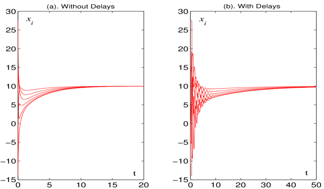
Figure 6: Simulation results of Example 3.2 without delays and with delays. Initial conditions, chosen randomly, are the same for each simulation. In both cases, group agreement to the leader value ${\bf x}_{0}$ is reached.

Note that even if ${\bf x}_{0}$ is not a constant, i.e., the dynamics of the $i$th element is given as

$$\dot{\bf x}_{i}=\sum_{j\in{\mathcal{N}}_{i}}{\bf K}_{ji}\ ({\bf x}_{j}(t-T_{ji})-{\bf x}_{i}(t))+\gamma_{i}\ {\bf K}_{0i}\ ({\bf x}_{0}(t-T_{0i})-{\bf x}_{i}(t))$$

the whole system is still asymptotically contracting according to exactly the same proof. Regardless of the initial conditions, all solutions will converge to a particular one, which in this case depends on the dynamics of ${\bf x}_{0}$ and the explicit values of the delays. Moreover, if ${\bf x}_{0}$ is periodic, as one of the main properties of contraction [11], all the followers’ state ${\bf x}_{i}$ will tend to be periodic with the same period as ${\bf x}_{0}$.

• Example 3.3

  : Consider the leader-followers network in Example 3.2 again. We set everything the same except that the leader’s states is not constant. Instead, we choose

  $${\bf x}_{0}=10\ \sin(\frac{t}{2})$$

  The whole system is still asymptotically contracting regardless of the delays. Simulation results are plotted in Figure 7. $\Box$

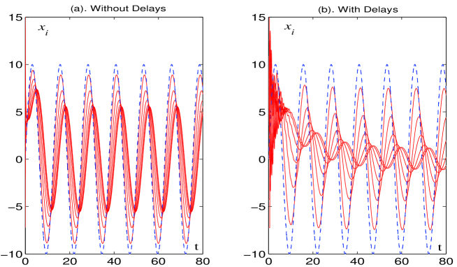
Figure 7: Simulation results of Example 3.3 without delays and with delays. In both plots, the dashed curve is the state of the leader while the solid ones are the states of the followers, which converge to a periodic solution in both cases regardless of the initial conditions.

3.3 Discrete-Time Models

Simplified wave variables can also be applied to study time-delayed communications in discrete-time models. Consider the model of flocking or schooling studied in [9, 30], where each element’s state is updated according to the discrete-time law that computes the average of its neighbors’ states plus its own state, i.e.,

$$x_{i}(t+1)\ =\ \frac{1}{1+n_{i}}\ (\ x_{i}(t)\ +\ \sum_{j\in{\mathcal{N}}_{i}}x_{j}(t)\ )\ \ \ \ \ \ \ \ \ \ \ \ \ \ \ \ \ \ \ \ \ i=1,\ldots,n$$ (18)

or, in an equivalent form

$$x_{i}(t+1)\ =\ x_{i}(t)\ +\ \frac{1}{1+n_{i}}\ \sum_{j\in{\mathcal{N}}_{i}}\ (\ x_{j}(t)\ -\ x_{i}(t)\ )$$

In fact, in equation (18), there is no difference if $x_{i}$ is a scalar or a vector. For notation simplicity we set $x_{i}$ as a scalar, but our analysis can be extended directly to the vector case. In equation (18), $\ t\$ is the index of the updating steps, so that its value is always an integer. $\ {\mathcal{N}}_{i}\$ denotes the set of the active neighbors of element $i$, which for instance can be defined as the set of the nearest neighbors within a certain distance $r$ around $i$. $\ n_{i}\$ equals to the number of the neighbors of element $i$. As proved in [9], the whole system (18) will tend to reach a group agreement if the network is connected in a very loose sense.

Assume now that time delays are non-negligible in communications. The update law of the $i$th element changes to

$$x_{i}(t+1)\ =\ x_{i}(t)\ +\ \frac{1}{1+n_{i}}\ \sum_{j\in{\mathcal{N}}_{i}}\ (\ x_{j}(t-T_{ji})\ -\ x_{i}(t)\ )$$ (19)

where the delay value $T_{ji}$ is an integer based on the number of updating steps. As in previous sections, $T_{ji}$ could be different for different communication links, or even different along opposite directions on the same link. For our later analysis, here we make a few assumptions: all elements update their states synchronously, and the time interval between any two updating steps is a constant; the network structure is fixed and always connected, which implies that $\forall i$, $n_{i}$ is a positive integer; the value of neighborship radius $r$ is unique through the whole network, which leads to the fact that all interactions are bidirectional.

Theorem 5

Consider $n$ coupled elements (19) with time-delayed communications. Regardless of the explicit values of the delays, the whole system will tend to reach a group agreement $x_{1}(t)=\cdots=x_{n}(t)$ asymptotically.

Proof: See Appendix. $\Box$

Similarly, consider the discrete-time model of a cooperating group with a leader-followers structure, where the dynamics of the $i$th follower is given as

$$x_{i}(t+1) = \frac{1}{1+n_{i}+\gamma_{i}}\ (\ x_{i}(t)\ +\ \sum_{j\in{\mathcal{N}}_{i}}\ x_{j}(t-T_{ji})\ +\ \gamma_{i}x_{0}\ )$$

$$= \frac{1+n_{i}}{1+n_{i}+\gamma_{i}}x_{i}(t)\ +\ \sum_{j\in{\mathcal{N}}_{i}}\ \tau_{ji}(t)\ +\ \frac{\gamma_{i}}{1+n_{i}+\gamma_{i}}x_{0}$$

and $\tau_{ji}$ is defined as in (Appendix: Proof of Theorem 5) with $k_{i}=1+n_{i}+\gamma_{i}$ and $\gamma_{i}=0$ or $1$. One easily shows that a very similar analysis leads to the same result as that of Theorem 4.

4 Concluding Remarks

Modified wave variables are analyzed in this paper, and are shown to yield effective tools for contraction analysis of interacting systems with time-delayed feedback communications. Future work on time-delays includes the development of analysis tools for general nonlinear systems, coupled networks with switching topologies, and time-varying time delays.

Appendix: Proof of Theorem 5

Equation (19) can be transformed to

$$x_{i}(t+1)\ =\ x_{i}(t)\ +\ \sum_{j\in{\mathcal{N}}_{i}}\tau_{ji}(t)$$

where the wave variables are defined as

$$u_{ji}=x_{i}\ +\ k_{i}\tau_{ji}\ \ \ \ \ \ \ \ \ \ \ \ \ \ \ \ v_{ij}=x_{i}$$

and $k_{i}=1+n_{i}$. Note that compared to (14), here we have ${\bf G}_{ij}={\bf G}_{ji}=1$ (the cooperation law could be extended to a more general form). Define

$$V(t)\ =\ \sum_{i=1}^{n}k_{i}\delta x_{i}^{2}(t)\ +\ \sum_{(i,j)\in{\mathcal{N}}}\ V_{i,j}(t)$$

where $\forall(i,j)\in{\mathcal{N}}=\cup_{i=1}^{n}{\mathcal{N}}_{i}$

$$V_{i,j}(t)\ =\ \sum_{\epsilon=t-1-T_{ij}}^{t-1}\delta v_{ij}^{2}(\epsilon)\ +\ \sum_{\epsilon=t-1-T_{ji}}^{t-1}\delta v_{ji}^{2}(\epsilon)\ -\ \sum_{\epsilon=-T_{ij}}^{0}\delta v_{ij}^{2}(\epsilon)\ -\ \sum_{\epsilon=-T_{ji}}^{0}\delta v_{ji}^{2}(\epsilon)$$

and therefore

$$V_{i,j}(t) = \sum_{\epsilon=0}^{t-1}(\ \delta v_{ij}^{2}(\epsilon)\ -\ \delta u_{ji}^{2}(\epsilon)\ +\ \delta v_{ji}^{2}(\epsilon)\ -\ \delta u_{ij}^{2}(\epsilon)\ )$$

$$= -\ \sum_{\epsilon=0}^{t-1}(\ 2k_{i}\delta x_{i}\delta\tau_{ji}(\epsilon)\ +\ k_{i}^{2}\delta\tau_{ji}^{2}(\epsilon)\ +\ 2k_{j}\delta x_{j}\delta\tau_{ij}(\epsilon)\ +\ k_{j}^{2}\delta\tau_{ij}^{2}(\epsilon)\ )$$

Since

$$\sum_{(i,j)\in{\mathcal{N}}}\big{(}V_{i,j}(t+1)\ -\ V_{i,j}(t)\big{)} = -\sum_{(i,j)\in{\mathcal{N}}}\ (\ 2k_{i}\delta x_{i}\delta\tau_{ji}(t)\ +\ k_{i}^{2}\delta\tau_{ji}^{2}(t)\ +\ 2k_{j}\delta x_{j}\delta\tau_{ij}(t)\ +\ k_{j}^{2}\delta\tau_{ij}^{2}(t)\ )$$

$$= -\sum_{i=1}^{n}\ (\ 2k_{i}\sum_{j\in{\mathcal{N}}_{i}}\delta x_{i}\delta\tau_{ji}(t)\ +\ k_{i}^{2}\sum_{j\in{\mathcal{N}}_{i}}\delta\tau_{ji}^{2}(t)\ )$$

one has

$$V(t+1) = \sum_{i=1}^{n}k_{i}(\ \delta x_{i}(t)\ +\ \sum_{j\in{\mathcal{N}}_{i}}\delta\tau_{ji}(t)\ )^{2}\ +\ \sum_{(i,j)\in{\mathcal{N}}}\ V_{i,j}(t+1)$$

$$= V(t)\ +\ \sum_{i=1}^{n}k_{i}\ (\ (\ \sum_{j\in{\mathcal{N}}_{i}}\delta\tau_{ji}(t)\ )^{2}\ -\ k_{i}\sum_{j\in{\mathcal{N}}_{i}}\delta\tau_{ji}^{2}(t)\ )$$

Note that

$$(\ \sum_{j\in{\mathcal{N}}_{i}}\delta\tau_{ji}\ )^{2}\ -\ k_{i}\sum_{j\in{\mathcal{N}}_{i}}\delta\tau_{ji}^{2} = \delta\Gamma_{i}^{T}\left[\begin{array}[]{ccc}1&\cdots&1\\ \vdots&\ddots&\vdots\\ 1&\cdots&1\end{array}\right]\delta\Gamma_{i}\ -\ k_{i}\delta\Gamma_{i}^{T}\delta\Gamma_{i}$$

$$= \delta\Gamma_{i}^{T}\left[\begin{array}[]{cccc}-n_{i}&1&\cdots&1\\ 1&-n_{i}&\cdots&1\\ \vdots&\vdots&\ddots&\vdots\\ 1&1&\cdots&-n_{i}\end{array}\right]\delta\Gamma_{i}$$

$$\leq -\ \delta\Gamma_{i}^{T}\delta\Gamma_{i}\ =\ -\ \sum_{j\in{\mathcal{N}}_{i}}\delta\tau_{ji}^{2}$$

where $\ \delta\Gamma_{i}=[\cdots,\ \delta\tau_{ji},\ \cdots]^{T}\in\mathbb{R}^{n_{i}}\$, so that

$$V(t+1)\ \leq\ V(t)\ -\ \sum_{i=1}^{n}k_{i}\ \sum_{j\in{\mathcal{N}}_{i}}\delta\tau_{ji}^{2}(t)$$

Since $V$ is lower bounded it converges to a finite limit as $t\rightarrow+\infty$, which implies that $\forall(i,j)\in{\mathcal{N}}$, $\delta\tau_{ji}$ tends to zero, which in turn implies that $\forall i$, $\delta x_{i}$ tends to zero. The rest of the proof is then similar to that of Theorem 3.

References

• [1] Aghannan, N., Rouchon, P., An Intrinsic Observer for a Class of Lagrangian Systems, I.E.E.E. Trans. Aut. Control, 48(6) (2003).
• [2] Anderson, R., and Spong, M.W. (1989) Bilateral Control of Teleoperators, IEEE Trans. Aut. Contr., 34(5),494-501
• [3] Chopra, N., Spong, M.W., Hirche, S., and Buss, M. (2003) Bilateral Teleoperation over the Internet: the Time Varying Delay Problem, Proceedings of the American Control Conference, Denver, CO.
• [4] Chu, T., Wang, L., and Mu, S. (2004) Collective Behavior Analysis of an Anisotropic Swarm Model, The $16$th International Symposium on Mathematical Theory of Networks and Systems, Belgium
• [5] Egeland, O., Kristiansen, E., and Nguyen, T.D., Observers for Euler-Bernoulli Beam with Hydraulic Drive, I.E.E.E. Conf. Dec. Control (2001).
• [6] Fierro, R., Song, P., Das, A., and Kumar, V. (2002) Cooperative Control of Robot Formations, in Cooperative Control and Optimization: Series on Applied Optimization, Kluwer Academic Press, 79-93
• [7] Godsil, C., and Royle, G. (2001) Algebraic Graph Theory, Springer
• [8] Horn, R.A., and Johnson, C.R. (1985) Matrix Analysis, Cambridge University Press
• [9] Jadbabaie, A., Lin, J., and Morse, A.S. (2003) Coordination of Groups of Mobile Autonomous Agents Using Nearest Neighbor Rules, IEEE Transactions on Automatic Control, 48:988-1001
• [10] Leonard, N.E., and Fiorelli, E. (2001) Virtual Leaders, Artificial Potentials and Coordinated Control of Groups, 40th IEEE Conference on Decision and Control
• [11] Lohmiller, W., and Slotine, J.J.E. (1998) On Contraction Analysis for Nonlinear Systems, Automatica, 34(6)
• [12] Lohmiller, W. (1999) Contraction Analysis of Nonlinear Systems, Ph.D. Thesis, Department of Mechanical Engineering, MIT
• [13] Lohmiller, W., and Slotine, J.J.E. (2000) Control System Design for Mechanical Systems Using Contraction Theory, IEEE Trans. Aut. Control, 45(5)
• [14] Moreau, L (2004) Stability of Continuous-Time Distributed Consensus Algorithms, submitted
• [15] Niemeyer, G., and Slotine, J.J.E. (2001) Towards Bilateral Internet Teleoperation, in Beyond Webcams: An Introduction to Internet Telerobotics, eds. K. Goldberg and R. Siegwart, The MIT Press, Cambridge, MA.
• [16] Niemeyer, G., and Slotine, J.J.E. (1998) Towards Force-Reflecting Teleoperation Over the Internet, IEEE Conf. on Robotics and Automation, Leuven, Belgium
• [17] Niemeyer, G., and Slotine, J.J.E. (1991), Stable Adaptive Teleoperation, IEEE J. of Oceanic Engineering, 16(1)
• [18] Olfati-Saber, R., and Murray, R.M. (2003) Consensus Protocols for Networks of Dynamic Agents, American Control Conference, Denver, Colorado
• [19] Olfati-Saber, R., and Murray, R.M. (2004) Consensus Problems in Networks of Agents with Switching Topology and Time-Delays, to appear in the special issue of the IEEE Transactions On Automatic Control on Networked Control Systems
• [20] Pikovsky, A., Rosenblum, M., and Kurths, J. (2003) Synchronization: A Universal Concept in Nonlinear Sciences, Cambridge University Press
• [21] Reynolds, C. (1987) Flocks, Birds, and Schools: a Distributed Behavioral Model, Computer Graphics, 21:25-34
• [22] Slotine, J.J.E. (2003) Modular Stability Tools for Distributed Computation and Control, International Journal of Adaptive Control and Signal Processing, 17(6)
• [23] Slotine, J.J.E., and Li, W. (1991) Applied Nonlinear Control, Prentice Hall
• [24] Slotine, J.J.E., and Lohmiller, W. (2001), Modularity, Evolution, and the Binding Problem: A View from Stability Theory, Neural Networks, 14(2)
• [25] Slotine, J.J.E., and Wang, W. (2003) A Study of Synchronization and Group Cooperation Using Partial Contraction Theory, Block Island Workshop on Cooperative Control, Kumar V. Editor, Springer-Verlag
• [26] Slotine, J.J.E., Wang, W., and El-Rifai, K. (2004) Contraction Analysis of Synchronization in Networks of Nonlinearly Coupled Oscillators, Sixteenth International Symposium on Mathematical Theory of Networks and Systems, Belgium
• [27] Smale, S. (1976) A Mathematical Model of Two Cells via Turing’s Equation, in The Hopf Bifurcation and Its Applications, Spinger-Verlag, 354-367
• [28] Strogatz, S. (2003) Sync: The Emerging Science of Spontaneous Order, New York: Hyperion
• [29] Tanner, H., Jadbabaie, A., and Pappas, G.J. (2003) Coordination of Multiple Autonomous Vehicles, IEEE Mediterranian Conference on Control and Automation, Rhodes, Greece
• [30] Vicsek, T., Czirók, A., Ben-Jacob, E., and Cohen I. (1995) Novel Type of Phase Transition in a System of Self-Driven Particles, Phys. Rev. Lett., 75:1226-1229
• [31] Wang, W., and Slotine, J.J.E. (2003) On Partial Contraction Analysis for Coupled Nonlinear Oscillators, NSL Report 030100, MIT, Cambridge, MA, to be published in Biological Cybernetics.
• [32] Wang, W., and Slotine, J.J.E. (2004) Where To Go and How To Go: a Theoretical Study of Different Leader Roles, NSL Report 040202, MIT, Cambridge, MA, submitted
• [33] Xie G., Wang L. (2004) Stability and Stabilization of Switched Linear Systems with State Delay: Continuous-Time Case, The $16$th International Symposium on Mathematical Theory of Networks and Systems, Belgium
• [34] Xie G., Wang L. (2004) Stability and Stabilization of Switched Linear Systems with State Delay: Discrete-Time Case, The $16$th International Symposium on Mathematical Theory of Networks and Systems, Belgium