Hyperelliptic Theta-Functions and Spectral Methods II

Abstract.

This is the second in a series of papers on the numerical treatment of hyperelliptic theta-functions with spectral methods. A code for the numerical evaluation of solutions to the Ernst equation on hyperelliptic surfaces of genus 2 is extended to arbitrary genus and general position of the branch points. The use of spectral approximations allows for an efficient calculation of all characteristic quantities of the Riemann surface with high precision even in almost degenerate situations as in the solitonic limit where the branch points coincide pairwise. As an example we consider hyperelliptic solutions to the Kadomtsev-Petviashvili and the Korteweg-de Vries equation. Tests of the numerics using identities for periods on the Riemann surface and the differential equations are performed. It is shown that an accuracy of the order of machine precision can be achieved.

1. Introduction

Solutions to integrable differential equations in terms of theta-functions were introduced at the beginning of the seventies, see [1] for an account of the history. In general, they describe periodic or quasi-periodic solutions. In contrast to the well-known solitonic solutions in terms of elementary functions, the theta-functions are special transcendental functions defined on some Riemann surface. All quantities entering the solution are given in explicit form via integrals which depend implicitly on the branch points of the Riemann surface. A full understanding of the functional dependence on these parameters seems to be only possible numerically. Algorithms have been developed to establish such relations for rather general Riemann surfaces as in [20] or via Schottky uniformization (see [1, 2]), which have been incorporated successively in numerical and symbolic codes, see [4, 5, 7, 13, 14, 19] and references therein (the first two references are distributed along with Maple 6, respectively Maple 8, and as a Java implementation [21]).

These codes are convenient to study theta-functional solutions on a given surface. To establish the dependence of the characteristic quantities of a Riemann surface on the branch points, an efficient calculation of the periods is necessary. This is especially true if the modular dependence of the theta-functions is of interest as in the case of theta-functional solutions to the Ernst equation [8] in [15, 16].

In [12], henceforth referred to as I, we have presented a code for the numerical treatment of hyperelliptic solutions to the Ernst equation on a surface of genus 2. The integrals entering the solution are calculated by expanding the integrands as a series of Chebyshev polynomials using a Fast Cosine Transformation in MATLAB and then integrating the polynomials in an appropriate way. In the present article, this code is extended to hyperelliptic surfaces of arbitrary genus and of branch points in general position. As an example we consider hyperelliptic solutions to the Kadomtsev-Petviashvili (KP) equation and the Korteweg-de Vries (KdV) equation. The precision of the numerical evaluation is tested by checking identities for periods on Riemann surfaces and the differential equations. We show that an accuracy of the order of machine precision ($\sim 10^{-14}$) can be achieved for branch points in general position with 32 polynomials and in the case of almost degenerate surfaces which occurs e.g. in the well-known solitonic limit with at most 256 polynomials. Consequently the solitonic limit can be carried out numerically with machine precision which will be shown at the example of the 2-soliton solution to the KdV equation. This makes it possible to study the parameter space for hyperelliptic surfaces numerically.

This paper is a sequel to I which was devoted to genus 2 solutions to the Ernst equation. We will only briefly repeat the methods already outlined there and refer the reader to I for details. The article is organized as follows: in section 2 we collect useful facts on the KP and the KdV equation and hyperelliptic Riemann surfaces, in section 3 we summarize basic features of spectral methods and explain our implementation of various quantities. The calculation of the periods of the hyperelliptic surface is performed together with tests of the precision of the numerics. The theta-series is approximated as in [5] as a finite sum. It is checked numerically how well the theta-functional solution solves the differential equation. In section 4 we present several examples of hyperelliptic solutions to the KP and the KdV equation in general cases and in almost solitonic situations. In section 5 we add some concluding remarks.

2. KP and KdV equation and hyperelliptic Riemann surfaces

The KP equation for the real valued potential $u$ depending on the three real coordinates $(x,y,t)$ can be written in the form

(1) $$3u_{yy}+\partial_{x}(6uu_{x}+u_{xxx}-4u_{t})=0.$$

The completely integrable equation has a physical interpretation as describing the propagation of weakly two-dimensional waves of small amplitude in shallow water as well as similar physical processes, see [1]. We note that there is a variant of the KP equation having a different sign of the $u_{xxx}$-term which will not be considered here.

Algebro-geometric solutions to the KP equation can be given on an arbitrary Riemann surface. Here we will only consider hyperelliptic surfaces $\Sigma_{g}$ of genus $g$ corresponding to the plane algebraic curve

(2) $$\mu^{2}=\prod_{i=1}^{g+1}(K-E_{i})(K-F_{i})=:K^{2g+2}-S_{1}K^{2g+1}+S_{2}K^{2g}+\ldots,$$

where we have defined the symmetric (in the branch points) functions $S_{n}$, $n=1,\ldots,2g+2$. We will concentrate on real surfaces with real branch points $E_{i}$, $F_{i}$. The branch points are ordered, $E_{1}<F_{1}<\ldots<E_{g+1}<F_{g+1}$.

Hyperelliptic Riemann surfaces are important since they show up in the context of algebro-geometric solutions of various integrable equations such as KdV, Sine-Gordon and Ernst. Whereas it is a non-trivial problem to find a basis for the holomorphic differentials on general surfaces (see e.g. [4]), it is given in the hyperelliptic case (see e.g. [1]) by

(3) $$\left(\frac{dK}{\mu},\frac{KdK}{\mu},\ldots,\frac{K^{g-1}dK}{\mu}\right),$$

which is the main simplification in the use of these surfaces. We introduce on $\Sigma_{g}$ a canonical basis of cycles $(a_{k},b_{k})$, $k=1,\ldots,n$ as in Fig. 1. The holomorphic differentials $d\omega_{k}$ are another basis in the space of holomorphic differentials which is normalized by the condition on the $a$-periods

(4) $$\int_{a_{l}}d\omega_{k}=2\pi{\mathrm{i}}\delta_{lk}.$$

This fixes the $d\omega_{k}$ uniquely given the system of cycles. The corresponding matrix of $b$-periods is given by $\mathbf{B}_{lk}=\int_{b_{l}}d\omega_{k}$. The matrix $\mathbf{B}$ is a so-called Riemann matrix, i.e. it is symmetric and has a negative definite real part.

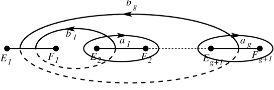
Figure 1. Canonical cycles.

The surfaces we consider here are real, i.e. they have an anti-holomorphic involution $\tau:\Sigma_{g}\to\Sigma_{g}$ with $\tau^{2}=1$. The basis of the homology is chosen to have the property

(5) $$\tau b_{j}=b_{j},\quad\tau a_{j}=-a_{j},\quad j=1,\ldots,g.$$

This implies for the normalized holomorphic differentials $d\omega_{j}$ the reality condition

(6) $$\tau d\omega_{j}=\overline{d\omega_{j}}.$$

The matrix of $b$-periods is real in this case.

The theta-function with characteristics corresponding to the curve $\Sigma_{g}$ is given by

(7) $$\Theta_{\mathbf{p}\mathbf{q}}(\mathbf{x}|\mathbf{B})=\sum_{\mathbf{n}\in\mathbb{Z}^{g}}\exp\left\{\frac{1}{2}\langle\mathbf{B}(\mathbf{p}+\mathbf{n}),(\mathbf{p}+\mathbf{n})\rangle+\langle\mathbf{p}+\mathbf{n},2\pi{\mathrm{i}}\,\mathbf{q}+\mathbf{x}\rangle\right\},$$

where $\mathbf{x}\in\mathbb{C}^{g}$ is the argument and $\mathbf{p},\mathbf{q}\in\mathbb{C}^{g}$ are the characteristics. We will only consider half-integer characteristics in the following. The theta-function with characteristics is, up to an exponential factor, equivalent to the theta-function with zero characteristic (this is the Riemann theta-function, denoted with $\Theta$) and shifted argument,

(8) $$\Theta_{\mathbf{p}\mathbf{q}}(\mathbf{x}|\mathbf{B})=\Theta(\mathbf{x}+\mathbf{B}\mathbf{p}+2\pi{\mathrm{i}}\,\mathbf{q})\exp\left\{\frac{1}{2}\langle\mathbf{B}\mathbf{p},\mathbf{p}\rangle+\langle\mathbf{p},2\pi{\mathrm{i}}\,\mathbf{q}+\mathbf{x}\rangle\right\}.$$

It has the periodicity properties

(9) $$\Theta_{\mathbf{p}\mathbf{q}}(\mathbf{z}+2\pi{\mathrm{i}}\,\mathbf{e}_{j})=e^{2\pi ip_{j}}\Theta_{\mathbf{p}\mathbf{q}}(\mathbf{z}),\quad\Theta_{\mathbf{p}\mathbf{q}}(\mathbf{z}+\mathbf{B}\mathbf{e}_{j})=e^{-2\pi{\mathrm{i}}\,q_{j}-z_{j}-\frac{1}{2}B_{jj}}\Theta_{\mathbf{p}\mathbf{q}}(\mathbf{z}),$$

where $\mathbf{e}_{j}$ is the $g$-dimensional vector consisting of zeros except for a 1 in jth position.

The differentials of the second kind needed here have a pole of order $l=1,2,3$ at infinity. They will be denoted by $d\Omega_{l}$. The Laurent expansion of the corresponding integrals is of the form

(10) $$\int_{\infty}^{P}d\Omega_{l}=k^{l}+o(1),$$

where $k$ is the local parameter in the vicinity of infinity. The singularity structure characterizes the differentials only up to an arbitrary linear combination of holomorphic differentials. This arbitrariness is eliminated by imposing the condition that all $a$-periods vanish. The normalized differentials satisfy the reality conditions $\tau d\Omega_{l}=\overline{d\Omega_{l}}$. The vectors of $b$-periods of these differentials are denoted by

(11) $$U_{n}=\int_{b_{n}}d\Omega_{1},\quad V_{n}=\int_{b_{n}}d\Omega_{2},\quad W_{n}=\int_{b_{n}}d\Omega_{3}.$$

The periods are real under the above conditions. For later use we define the constant $c$ via the expansion of the integral $\Omega_{1}$,

(12) $$\int_{\infty}^{P}d\Omega_{1}=k-\frac{c}{k}+O(k^{-2}).$$

The differentials of the second kind $d\Omega_{i}$ are given explicitly on $\Sigma_{g}$ by

(13) $$d\Omega_{1}=\frac{K^{g+1}-\frac{1}{2}S_{1}K^{g}+c_{1}K^{g-1}+\ldots+c_{g}}{2\mu(K)}\,dK,$$

where the $c_{l}$ are determined by the condition of vanishing $a$-periods,

(14) $$d\Omega_{2}=\frac{K^{g+2}-\frac{1}{2}S_{1}K^{g+1}-(\frac{1}{8}S_{1}^{2}-\frac{1}{2}S_{2})K^{g}}{\mu(K)}\,dK+\ldots,$$

and

(15) $$d\Omega_{3}=\frac{3}{2}\frac{K^{g+3}-\frac{1}{2}S_{1}K^{g+2}-(\frac{1}{8}S_{1}^{2}-\frac{1}{2}S_{2})K^{g+1}-(\frac{1}{16}S_{1}^{3}-\frac{1}{4}S_{1}S_{2}+\frac{1}{2}S_{3})K^{g}}{\mu(K)}dK+\ldots,$$

where $\ldots$ denotes the holomorphic differentials leading to vanishing $a$-periods. For the constant $c$, we get

(16) $$c=\frac{S_{1}^{2}}{8}-\frac{S_{2}}{2}+c_{1}.$$

It is well known that the $b$-periods of normalized differentials of the second kind can be expressed in terms of expansions of the holomorphic differentials in the vicinity of the singularity (see e.g. [1]). We write the holomorphic differentials in the vicinity of some point $a$ in the form

(17) $$d\omega=\sum_{n=0}^{\infty}\mathbf{v}_{n}\frac{t^{n}}{n!}dt,$$

where $t$ is the local parameter in the vicinity of $a$. If we choose $a=\infty^{+}$ (the infinite point in the upper sheet), we have

(18) $$\mathbf{v}_{0}=\mathbf{U},\quad\mathbf{v}_{1}=\mathbf{V},\quad\mathbf{v}_{2}=\mathbf{W}/2.$$

Thus, the periods $\mathbf{U}$, $\mathbf{V}$ and $\mathbf{W}$ can be calculated as the $b$-periods of the differentials $d\Omega_{i}$, $i=1,2,3$, or via an expansion of the holomorphic differentials.

Solutions to the KP equation on the above Riemann surfaces are given by the generalization of the Its-Matveev formula for the KdV equation (see e.g. [17])

(19) $$u=2\partial_{x}^{2}\ln\Theta(\mathbf{U}x+\mathbf{V}y+\mathbf{W}t+\mathbf{D})+2c,$$

where $\mathbf{D}\in\mathbb{C}^{g}$ is an arbitrary real vector. Because of (8) and the second logarithmic derivative in (19), the vector $\mathbf{D}$ can always be absorbed in the form of a real characteristic. By a coordinate change $x\to x+tc/3$ one can change a solution $u$ to the KP equation by $-2c$.

The reality of the argument of the theta-function implies that the theta-function which is an entire function does not vanish. This can be seen from the following argument for the elliptic case:

(20) $$\Theta(x) = \sum_{m\in\mathbb{Z}}\exp\left(\frac{1}{2}m^{2}B+mx\right)$$

$$= 1+2\sum_{m\in\mathbb{N}}\exp\left(\frac{1}{2}m^{2}B\right)\cosh(mx)>0.$$

A generalization of the argument to higher genus is straightforward.

Probably the most elegant way to show that (19) provides a solution to the KP equation is the use of Fay’s trisecant identity [9]. This is an identity for theta-functions which holds for four arbitrary points on a Riemann surface, see [17] for details. Here we need the identity in the limit that all four points coincide which leads to an identity for derivatives of theta-functions. We introduce the directional derivatives on $\mathbb{C}^{g}$ ($\nabla$ acts on $\mathbf{z}\in\mathbb{C}^{g}$)

(21) $$D_{a}=\mathbf{v}_{0}\cdot\nabla,\quad D_{a}^{\prime}=\mathbf{v}_{1}\cdot\nabla,\quad D_{a}^{\prime\prime}=\mathbf{v}_{2}\cdot\nabla.$$

Then for an arbitrary vector $\mathbf{z}$ the following identity holds:

(22) $$\begin{split}D_{a}^{4}\ln\Theta(\mathbf{z})+6(D_{a}^{2}\ln\Theta(\mathbf{z}))^{2}+3D_{a}^{\prime}D_{a}^{\prime}\ln\Theta(\mathbf{z})-2D_{a}D_{a}^{\prime\prime}\ln\Theta(\mathbf{z})&\\ -24C_{1}D_{a}^{2}\ln\Theta(\mathbf{z})+12(10C_{2}-3C_{1}^{2})&=0.\end{split}$$

Here the constants $C_{1}$, $C_{2}$ turn up in the Taylor expansion of the differential $d\Omega_{1}$ from above ($a=\infty^{+}$),

(23) $$d\Omega_{1}=-\frac{1}{t^{2}}+2C_{1}-(6C_{1}^{2}-12C_{2})t^{2}+\ldots.$$

We put $u=2(D_{a}^{2}\ln\Theta(\mathbf{z})-2C_{1})$ and get for relation (22) after differentiation with $D_{a}^{2}$

(24) $$D_{a}(D_{a}^{3}u+6uD_{a}u-2D_{a}^{\prime\prime}u)+3D_{a}^{\prime}D_{a}^{\prime}u=0.$$

Because of (18) this equation is for $\mathbf{z}=\mathbf{U}x+\mathbf{V}y+\mathbf{W}t+\mathbf{D}$ equivalent to the KP equation.

2.1. Reduction to KdV equation and solitonic limit

If the hyperelliptic surface $\Sigma_{g}$ is branched at infinity, i.e. if $F_{g+1}\to\infty$ in (2), the integral $\Omega_{2}$ is single valued. Thus, all its $a$- and $b$-periods vanish which implies that there is no $y$-dependence in the formula (19). Then the KP equation reduces to the KdV equation,

(25) $$6uu_{x}+u_{xxx}-4u_{t}=0.$$

The hyperelliptic surface is now defined by the algebraic curve

(26) $$\mu^{2}=(K-E_{g+1})\prod_{i=1}^{g}(K-E_{i})(K-F_{i})=:K^{2g+1}-S_{1}K^{2g}+S_{2}K^{2g}-\ldots+S_{2g+1}.$$

All definitions apply as before. We use a cut-system of the form Fig. 1 where all $b$-cycles start at the cut $[E_{g+1},\infty]$ along the positive real axis.

As a local parameter at infinity we can use ${\mathrm{i}}\sqrt{\lambda}$. The differentials of the second kind we need here read

(27) $$d\Omega_{1}=\frac{{\mathrm{i}}d\lambda}{2\mu(\lambda)}(\lambda^{g}+c_{1}\lambda^{g-1}+\ldots c_{g}),$$

and

(28) $$d\Omega_{3}=-\frac{3{\mathrm{i}}d\lambda}{2\mu(\lambda)}(\lambda^{g+1}-\frac{1}{2}S_{1}\lambda^{g}+d_{1}\lambda^{g-1}+\ldots+d_{g}),$$

where the constants $c_{i}$ and $d_{i}$ are again defined by the condition that all $a$-periods of the above differentials vanish. Writing the normalized holomorphic differentials as

(29) $$d\omega_{n}=\sum_{k=1}^{g}\frac{c_{nk}\lambda^{g-k}}{\mu}d\lambda,$$

we get for the $b$-periods of the differentials of the second kind

(30) $$U_{n}=c_{n1},\quad W_{n}=c_{n2}+\frac{S_{1}}{2}c_{n1}.$$

The constant $c$ reads

(31) $$c=-\left(\frac{S_{1}}{2}+c_{1}\right).$$

An interesting limiting case of the theta-functional solutions on a genus $g$ surface is the so-called solitonic limit, see [1, 17]. In this case $E_{i}\to F_{i}$ for $i=1,\ldots,g$ which leads to the $g$-soliton solution. Since $g$ of the cuts collapse to double points, the diagonal elements of the Riemann matrix diverge in the used cut-system as $B_{ii}\sim 2\ln(F_{i}-E_{i})$ whereas all other $a$- and $b$-periods remain finite. The theta-series thus breaks down to a sum containing only elementary functions. To obtain the standard form of the $g$-soliton, we choose the vector $\mathbf{D}$ in (19) to correspond to the half-integer characteristic

(32) $$\frac{1}{2}\left[\begin{array}[]{ccc}1&\ldots&1\\ 0&\ldots&0\end{array}\right].$$

On an elliptic surface we get with the above relations for (19) the 1-soliton solution of KdV equation,

(33) $$u=\frac{U^{2}}{2\cosh^{2}\frac{z}{2}}+2c,\quad z=Ux+Wt,$$

where

(34) $$U=2\sqrt{E_{2}-E_{1}},\quad W=-2\sqrt{E_{2}-E_{1}}S_{1},\quad c=-\frac{E_{2}}{2}.$$

Similarly we get for the 2-soliton

(35) $$u-2c=\frac{U_{1}^{2}-U_{2}^{2}}{2}\frac{U_{1}^{2}\cosh^{2}\frac{z_{2}}{2}+U_{2}^{2}\sinh^{2}\frac{z_{1}}{2}}{(U_{1}\cosh\frac{z_{1}}{2}\cosh\frac{z_{2}}{2}-U_{2}\sinh\frac{z_{1}}{2}\sinh\frac{z_{2}}{2})^{2}},$$

where

(36) $$z_{i}=U_{i}x+W_{i}t,\quad U_{1}=2\sqrt{E_{3}-E_{1}},\quad U_{2}=2\sqrt{E_{3}-E_{2}},$$

and

(37) $$W_{1}=-\sqrt{E_{3}-E_{1}}(E_{3}+2E_{1}),\quad W_{2}=-\sqrt{E_{3}-E_{2}}(E_{3}+2E_{2}),\quad c=-\frac{E_{3}}{2}.$$

A generalization to higher genus is straight forward, see [18]. Formulas (34) and (35) hold also for the KP equation with the appropriate definition of $\mathbf{z}$ and $\mathbf{U}$.

3. Numerical implementations

The numerical task in this work is to approximate and evaluate analytically defined functions as accurately and efficiently as possible. To this end it is advantageous to use (pseudo-)spectral methods which are distinguished by their excellent approximation properties when applied to smooth functions. Here the functions are known to be analytic except for isolated points. In this section we explain the basic ideas behind the use of spectral methods and describe in detail how the theta-functions and its derivatives can be obtained to a high degree of accuracy.

3.1. Spectral approximation

The basic idea of spectral methods is to approximate a given function $f$ globally on its domain of definition by a linear combination

$$f\approx\sum_{k=0}^{N}a_{k}\phi_{k},$$

where the functions $\phi_{k}$ are taken from some class of functions which is chosen appropriately for the problem at hand. The spectral coefficients are determined by a so-called collocation method, i.e. by the condition that $f(x_{l})=\sum_{k=0}^{N}a_{k}\phi_{k}(x_{l})$ at selected points $(x_{l})_{l=0:N}$. Since we are interested in an approximation of functions defined on a finite interval, orthogonal polynomials, in particular Chebyshev $T_{n}(x)$ polynomials will be chosen. They are defined on the interval $I=[-1,1]$ by the relation

$$T_{n}(\cos(t))=\cos(nt),\text{where }x=\cos(t),\qquad t\in[0,\pi].$$

The Chebyshev polynomials are used because they have very good approximation properties and because one can use fast transform methods when computing the expansion coefficients from the function values provided one chooses the collocation points $x_{l}=\cos(\pi l/N)$ (see [10] and references therein).

Let us briefly summarize here some basic properties of Chebyshev polynomials: The addition theorems for sine and cosine imply the recursion relations

(38) $$\frac{T^{\prime}_{n+1}(x)}{n+1}-\frac{T^{\prime}_{n-1}(x)}{n-1}=2T_{n}(x)$$

for their derivatives. The Chebyshev polynomials are orthogonal on $I$ with respect to the hermitian inner product

$$\left<f,g\right>=\int_{-1}^{1}f(x)\bar{g}(x)\,\frac{dx}{\sqrt{1-x^{2}}}.$$

We have

(39) $$\left<T_{m},T_{n}\right>=c_{m}\frac{\pi}{2}\,\delta_{mn}$$

where $c_{0}=2$ and $c_{l}=1$ otherwise.

The fact that $f$ is approximated globally by a finite sum of polynomials allows us to express any operation applied to $f$ approximately in terms of the coefficients. Let us illustrate this in the case of integration. So we assume that $f=p_{N}=\sum_{n=0}^{N}a_{n}T_{n}$, and we want to find an approximation of the integral for $p_{N}$, i.e., the function

$$F(x)=\int_{-1}^{x}f(s)\,ds,$$

so that $F^{\prime}(x)=f(x)$. We make the ansatz $F(x)=\sum_{n=0}^{N}b_{n}\,T_{n}(x)$ and obtain the equation

$$F^{\prime}=\sum_{n=0}^{N}b_{n}\,T^{\prime}_{n}=\sum_{n=0}^{N}a_{n}T_{n}=f.$$

Expressing $T_{n}$ in terms of the $T^{\prime}_{n}$ using (38) and comparing coefficients determines all $b_{l}$ in terms of the $a_{n}$ except for $b_{0}$. This free constant is determined by the requirement that $F(-1)=0$. Thus, to find an approximation of the definite integral $\int_{-1}^{1}f(x)dx$ we proceed as described above, first computing the coefficients $a_{n}$ of $f$, computing the $b_{n}$ and then calculating the sum of the necessary coefficients.

3.2. Numerical treatment of the periods

The quantities entering formula (19) are the periods of certain differentials on the Riemann surface. The value of the theta-function is then approximated by a finite sum.

The periods of a hyperelliptic Riemann surface can be expressed as integrals between branch points. Since we need in our example the periods of the holomorphic differentials and differentials of the second kind with poles at $\infty^{\pm}$, we have to consider integrals of the form

(40) $$\int_{P_{i}}^{P_{j}}\frac{K^{n}dK}{\mu(K)},\quad n=0,\ldots,g+3,$$

where the $P_{j}$, $j=1,\ldots,2g+2$ denote the branch points of $\Sigma_{g}$.

We parametrize the straight line between the two branch points $P_{i}$ and $P_{j}$ by

$$K=\frac{1}{2}(P_{j}+P_{i})+\frac{t}{2}(P_{j}-P_{i})$$

to obtain the integral (40) in the normal form

(41) $$\int_{-1}^{1}\frac{\alpha_{0}+\alpha_{1}t+\ldots+\alpha_{g+3}t^{g+3}}{\sqrt{1-t^{2}}}\;H(t)\,dt,$$

where the $\alpha_{i}$ are complex constants and where $H(t)$ is a continuous (in fact, analytic) complex valued function on the interval $[-1,1]$. This form of the integral suggests to express the powers $t^{n}$ in the numerator in terms of Chebyshev polynomials and to approximate the function $H(t)$ by a linear combination of Chebyshev polynomials

$$H(t)=\sum_{n\geq 0}h_{n}T_{n}(t).$$

The integral is then calculated with the help of the orthogonality relation (39) of the Chebyshev polynomials.

This is the procedure used in I for general position of the branch points which can also be applied here for low genus. The problem is that there does not seem to be a direct way to express the terms $K^{n}$ in (40) after the linear transformation in terms of Chebyshev polynomials in $t$. This is an obstacle to the determination of the periods for general genus. Another problem are situations close to the solitonic limit. Since the cut-system Fig. 1 is adapted to this case, the $a$-periods do not lead to problems. For the $b$-periods, the function $H$ in the expression for $b_{i}$ (41) behaves like $1/\sqrt{t+E_{i}-F_{i}}$ near $t=0$. For $E_{i}\sim F_{i}$ this behavior is only satisfactorily approximated by a large number of polynomials. The use of a large number of polynomials however does not only require more computational resources but has the additional disadvantage of introducing larger rounding errors. It is therefore worthwhile to reformulate the problem since a high number of polynomials would be necessary to obtain optimal accuracy in this case.

It is possible to address both problems in one approach. The idea is to use substitutions in the integrals (40) leading to a regular integrand. To determine the $a$-periods, we use

(42) $$K=\frac{E_{i}+F_{i}}{2}+\frac{F_{i}-E_{i}}{2}\cosh x.$$

After a linear transformation which transforms the integration path to the interval $[-1,1]$, the integral is computed with the Chebyshev integration routine sketched above. This also works in situations close to the solitonic limit. To treat the $b$-periods in this case, we split the integral from $F_{i}$ to $E_{i+1}$ in two integrals from $F_{i}$ to $(F_{i}+E_{i+1})/2$ and from $(F_{i}+E_{i+1})/2$ to $E_{i+1}$. In the former case we use the substitution (42) and

(43) $$K=\frac{E_{i+1}+F_{i+1}}{2}+\frac{F_{i+1}-E_{i+1}}{2}\cosh x$$

in the latter. These substitutions lead to a regular integrand even in situations close to the solitonic limit. After a linear transformation, the integrals are computed with the Chebyshev integration routine. The disadvantage of this approach is that the definition of the square root adapted to the cut-system in I via monomials cannot be used in the case of the above non-linear transformations. Here the root is chosen in a way that the integrand is a continuous function on the path of integration. This can be achieved in general for real branch points.

To test the numerics we use the fact that in our case the integral of any holomorphic differential along a contour surrounding the cut $[E_{1},F_{1}]$ in positive direction is equal to minus the sum of all $a$-periods of this integral. Since this condition is not implemented in the code it provides a strong test for the numerics. The symmetry of the Riemann matrix (the matrix of $b$-periods of the holomorphic differentials after normalization) can be used to estimate the error in the numerical evaluation of the $b$-periods. We define the function $err$ as the maximum of the norm of the difference in the $a$-periods discussed above and the difference of the off-diagonal elements of the Riemann matrix. Additional tests for the periods $\mathbf{U}$, $\mathbf{V}$ and $\mathbf{W}$ follow from (18). We show in Fig. 2 a genus 2 situation with the branch points $[-3,-2,-1,-1+\epsilon,1,1+\epsilon]$. It can be seen that 32 polynomials are sufficient in general position ($\epsilon=1$) to achieve optimal accuracy. Since MATLAB works with 16 digits, machine precision is in general limited to 14 digits due to rounding errors. These rounding errors are also the reason why the accuracy drops slightly when a higher number of polynomials is used.

Figure 2. Test of the numerics for the $a$-periods at several points in the space-time. The error is shown in dependence of the number $N$ of Chebyshev polynomials.

In an almost degenerate situation ($\epsilon=10^{-14}$), optimal accuracy is achieved with 128 polynomials. Note that all quantities entering (19) are within $10^{-14}$ and better equal to the limits given in (36) and (37). Thus the solitonic limit can be reached numerically with machine precision.

The above procedure to determine the periods can be directly implemented within MATLAB for arbitrary genus. Due to the efficient vectorization algorithms of MATLAB, the calculation of the periods with optimal accuracy takes only a second even for genus 10 on the used low-end computers. The limiting factor is here whether the matrix $A$ of $a$-periods is ill conditioned. This is the case if a considerable number of the entries of $A$ are of the order of the rounding error ($10^{-16}$). Thus due to the limited number of digits, the inversion of the matrix $A$ which is necessary to determine the Riemann matrix can only be carried out with reduced accuracy which is independent of the number of polynomials used in the spectral expansion. For large genus, this becomes the limiting factor in the determination of the Riemann matrix. For instance in the case of the genus 20 surface with branch points $[-21,20,\ldots,20]$, the identity for $a$-periods is satisfied with 32 polynomials up to $10^{-15}$, the symmetry of the Riemann matrix only up to $10^{-6}$ since the matrix $A$ is badly scaled. The calculation of the periods takes less than a second in this case.

3.3. Theta-functions

The calculation of the theta-functions below is applicable for arbitrary Riemann surfaces, it is not limited to the hyperelliptic case. The theta-series (7) for the Riemann theta-function (the theta-function in (7) with zero characteristic, theta-functions with characteristic follow from (8)) is approximated as the sum

(44) $$\Theta(\mathbf{x}|\mathbf{B})=\sum_{n_{1}=-N}^{N}\ldots\sum_{n_{g}=-N}^{N}\exp\left\{\frac{1}{2}\langle\mathbf{M},\mathbf{B}\mathbf{M}\rangle+\langle\mathbf{M},\mathbf{x}\rangle\right\},$$

where $\mathbf{M}$ is a vector in $\mathbb{Z}^{g}$ with the components $n_{1},\ldots,n_{g}$. We use the periodicity properties of the theta-function (9) to minimize the absolute value of $x$. The value of $N$ is determined by the condition that terms in the series (7) for $n>N$ are strictly smaller than some threshold value $\epsilon$ which is taken to be of the order of $10^{-16}$. To this end we determine the eigenvalues of $\mathbf{B}$ and demand that

(45) $$N>-\frac{1}{gB_{max}}\left(||\mathbf{x}||+\sqrt{||\mathbf{x}||^{2}+2\ln\epsilon gB_{max}}\right),$$

where $B_{max}$ is the real part of the eigenvalue with maximal real part ($\mathbf{B}$ is negative definite). Similar formulas can be obtained for theta-derivatives. For a more sophisticated analysis of theta summations see [7, 5]. In the studied examples we found values of $N$ between 2 and 40. If the eigenvalues of $\mathbf{B}$ differ by more than an order of magnitude which can happen close to partial degeneration of the surface, a summation over an ellipse rather than over a sphere in the hypercube $(n_{1},\ldots,n_{2g})$, i.e. different limiting values for the $n_{i}$ as in [5] could be more efficient. The summation over the hypercube has, however, the advantage that it can be implemented in MATLAB for arbitrary genus. In addition it makes full use of MATLAB’s vectorization algorithms outlined below. Thus it is questionable whether a summation over an ellipse would be more efficient in terms of computation time in this setting.

Here we made use of MATLAB’s efficient way to handle matrices. We generate a $2N+1$-dimensional array containing all possible index combinations and thus all components in the sum (44) which is then summed. To illustrate this we consider the simple example of genus 2 with $N=2$. The summation indices are written as $(2N+1)\times(2N+1)$-matrices since $g=2$. Each of these matrices contains $2N+1$ copies of the vector with integers $-(2N+1),\ldots,2N+1$. $N_{2}$ is the transposed matrix of $N_{1}$. Explicitly, we have

(46) $$N_{1}=\left(\begin{array}[]{ccccc}2&2&2&2&2\\ 1&1&1&1&1\\ 0&0&0&0&0\\ -1&-1&-1&-1&-1\\ -2&-2&-2&-2&-2\end{array}\right),\quad N_{2}=\left(\begin{array}[]{ccccc}2&1&0&-1&-2\\ 2&1&0&-1&-2\\ 2&1&0&-1&-2\\ 2&1&0&-1&-2\\ 2&1&0&-1&-2\end{array}\right).$$

The terms in the sum (44) can thus be written in matrix form

(47) $$\exp\left(\frac{1}{2}N_{1}\star N_{1}B_{11}+N_{1}\star N_{2}B_{12}+\frac{1}{2}N_{2}\star N_{2}B_{22}+N_{1}\star x_{1}+N_{2}\star x_{2}\right),$$

where the operation $N_{1}\star N_{2}$ denotes that each element of $N_{1}$ is multiplied with the corresponding element of $N_{2}$. Thus, the argument of $\exp$ is a $(2N+1)\times(2N+1)$-dimensional matrix. Furthermore, the exponential function is understood to act not on the matrix but on each of its elements individually, producing a matrix of the same size. The approximate value of the theta-function is then obtained by summing up all the elements in (47).

The most time consuming operations are the determination of the bilinear terms involving the Riemann matrix. If one wants to calculate solutions to the KP equation, these terms only have to be determined once for a given surface. The integer $N$ is in this case fixed for the largest $||x||$ in the plot. We note that the summation is very fast even though the used determination of $N$ is rather crude. For instance in the case of genus $2$ with $N=100$, the calculation of the theta-function takes 0.1s on the used computers.

The limiting factor is here the available memory since arrays of the order $(2N+1)^{g}$ have to be multiplied with each other. On the used low-end computers we could deal with rather general genus 4 situations, but the limit was reached for genus 6 and $N=5$. The summation is still very efficient, the calculation of the bilinear terms and the determination of the coefficients took 16s in the latter case, the subsequent calculation of the linear terms in (47) and the summation, which have to be carried out for each value of $x$ and $t$, took roughly 4s. Thus the limitations we had to face were not due to the computing time but due to missing memory.

The quality of the theta summation can be checked directly by putting the approximate solution into the differential equation. The necessary derivatives of the theta-function entering the function $u$ and its derivatives can be calculated directly, e.g.

(48) $$\partial_{x}^{n}\Theta(\mathbf{z},\mathbf{B})=\sum_{n_{1}=-\tilde{N}}^{\tilde{N}}\ldots\sum_{n_{g}=-\tilde{N}}^{\tilde{N}}(\langle\mathbf{M},\mathbf{U}\rangle)^{n}\exp\left\{\frac{1}{2}\langle\mathbf{M},\mathbf{B}\mathbf{M}\rangle+\langle\mathbf{M},\mathbf{z}\rangle\right\},$$

where $\tilde{N}$ is determined as $N$ for the theta-series. The differential equations could be satisfied to the order of $10^{-13}$ and better. For the plots in the next section we use an accuracy of the order of $10^{-10}$. The error is mainly due to the fact that we did not choose $N$ big enough that also the terms in 6th derivative of the form (48) are of the order of the rounding error. For the solution only the second derivative is important. The accuracy of the solution is thus in general much higher as can be seen for instance in the solitonic example where the differential equation is satisfied to the order of $10^{-13}$, but the difference to the solitonic solution is smaller than $10^{-15}$.

4. Hyperelliptic solutions to KdV and KP equations

In this section we present plots of hyperelliptic solutions to the KdV and the KP equation as examples for the previously discussed code. Such plots can already be found in [17, 2] and [7]. We will show general situations as well as almost degenerate surfaces which are identical to their corresponding solitonic solution up to numerical accuracy. In all plots, the vector $\mathbf{D}$ in (19) is chosen to correspond to the characteristic (32).

It turns out that almost solitonic solutions take less computational resources. The calculation of the periods requires the use of more polynomials, but the most time-consuming part is the theta summation. Since the diagonal elements of the Riemann matrix diverge in this limit, less terms have to be considered in the summation. The generation of the plots is thus considerably faster than in general position of the branch points.

To begin we want to discuss plots of genus 2 solutions to the KdV equation. We consider a hyperelliptic surface of the form (26) with branch points $[-2,-2+\epsilon,-1,-1+\epsilon,3]$. In Fig. 3 we show the case for $\epsilon=10^{-14}$ which is identical to the $2$-soliton solution within machine precision. The difference between the shown plot and the solution (35) is actually less than $10^{-15}$. The one dimensional waves in shallow water are depicted in dependence on $x$ and $t$. It can be seen that a soliton coming from the right and traveling in negative $x$-direction has a collision with a soliton traveling in positive $x$-direction. At the collision the typical phase shift can be observed, otherwise the solitons are unaffected.

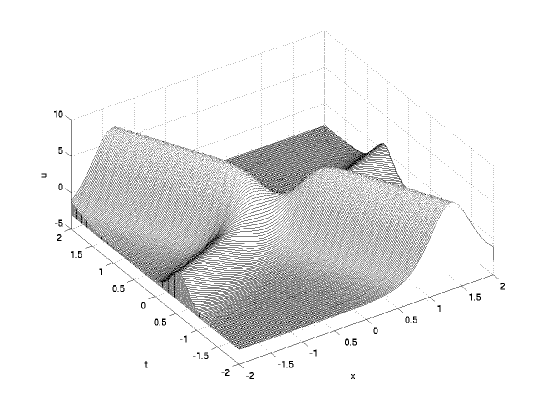
Figure 3. ‘Almost’ solitonic genus 2 solution to the KdV equation.

In Fig. 4 we show the case $\epsilon=1$. The almost periodic nature of the solution is clearly recognizable. The solution can be interpreted as an infinite train of solitons.

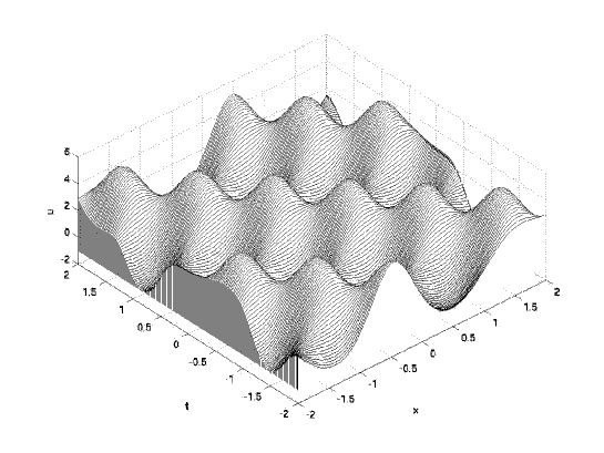
Figure 4. Almost periodic genus 2 solution to the KdV equation.

To obtain solutions on a surface of genus 6 we considered the surface with the branch points $[-6,-6+\epsilon,-4,-4+\epsilon,-2,-2+\epsilon,0,ep,2,2+\epsilon,4,4+\epsilon,6]$. The situation for $\epsilon=1$ is shown in Fig. 5. The depicted situation is at the limit imposed by memory on the used computer.

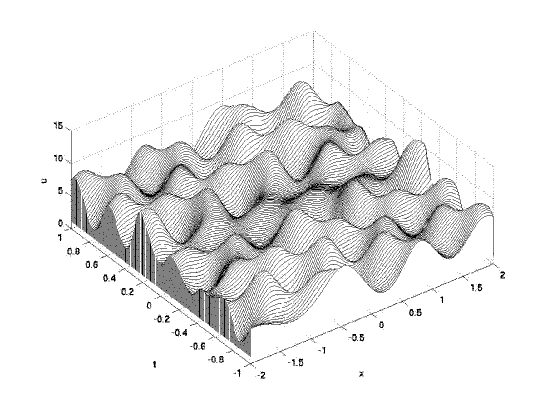
Figure 5. Almost periodic genus 6 solution to the KdV equation.

In Fig. 6 we show a solution of genus 6 in an almost solitonic situation. One can see the collision of 6 solitons at the center of the plot.

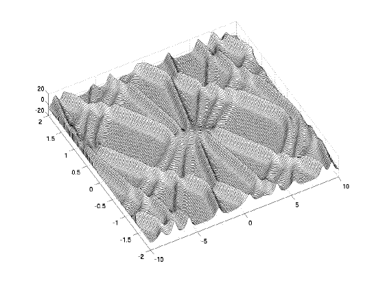
Figure 6. Almost solitonic genus 6 solution to the KdV equation.

A genus 4 solution of the KP equation is shown for fixed $t$ on the hyperelliptic surface with branch points $[-5,-4,-3,-3+\epsilon,-1,-1+\epsilon,1,1+\epsilon,3,3+\epsilon]$. In Fig. 7 we show the almost periodic situation for $\epsilon=1$.

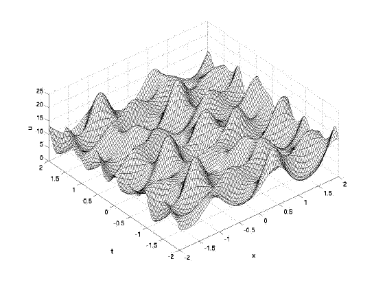
Figure 7. Almost periodic genus 4 solution to the KP equation.

The almost solitonic case with $\epsilon=0.001$ is shown in Fig. 8.

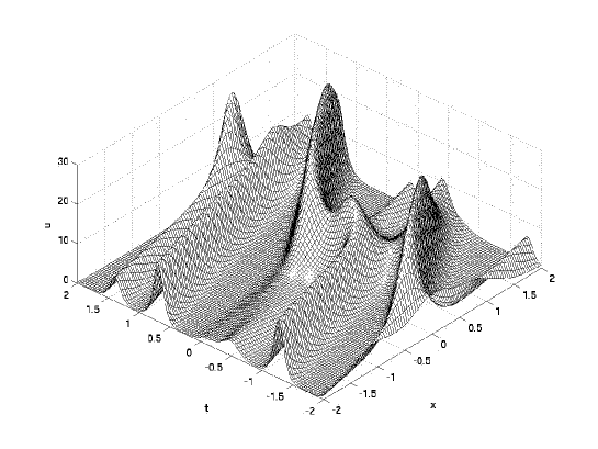
Figure 8. Almost solitonic genus 4 solution to the KP equation.

5. Conclusion

In this article we have presented a scheme based on spectral methods to treat hyperelliptic theta-functions of in principle arbitrary genus numerically. It was shown that an accuracy of the order of machine precision could be obtained with an efficient code. As shown, spectral methods are very convenient if analytic functions are approximated. Close to singularities such as the degeneration of the Riemann surface, analytic techniques must be used to obtain analytic integrands as in the discussed example. This made it possible to study the solitonic limit numerically within machine precision.

To consider the case that more than 2 branch points coincide, a higher number of polynomials or additional analytical techniques have to be used. As shown in I this makes it possible to study the parameter space of hyperelliptic surfaces including almost degenerate cases with at most 512 polynomials with maximal accuracy (here we used at most 128 polynomials). Both the calculation of the periods and the theta summation are very efficient. The limiting factor for the periods is the finite number of digits (16 in MATLAB) which leads to a drop of accuracy if the matrix of $a$-periods is ill-conditioned. The theta summation is limited by the available memory.

The presented numerical code is able to treat general hyperelliptic surfaces. The used method can in principle be extended to more general Riemann surfaces if the differentials are known explicitly as e.g. in the case of $Z_{N}$-curves.

References

- [1] E. D. Belokolos, A. I. Bobenko, V. Z. Enolskii, A. R. Its and V. B. Matveev, Algebro-Geometric Approach to Nonlinear Integrable Equations, Berlin: Springer, (1994).
- [2] A. Bobenko and L. Bordag, Periodic multiphase solutions to the Kadomtsev-Petviashvili equation, J.Phys. A: Math. Gen., 22, 1259 (1989).
- [3] W. L. Briggs and V. E. Henson, The DFT, an owner’s manual for the discrete Fourier transform, Siam Philadelphia, 1995.
- [4] B. Deconinck and M. van Hoeij, Computing Riemann matrices of algebraic curves, Physica D, 152-153, 28 (2001).
- [5] B. Deconinck, M. Heil, A. Bobenko, M. van Hoeij and M. Schmies, Computing Riemann Theta Functions, to appear in Mathematics of Computation.
- [6] B.A. Dubrovin, Theta functions and non-linear equations, Russ. Math. Surv. 36, 11 (1981).
- [7] B.A. Dubrovin, R. Flickinger and H. Segur, Three-phase solutions to the Kadomtsev-Petviashvili equation, Stud. Appli. Math., 99(2), 137 (1997).
- [8] F.J. Ernst, New formulation of the axially symmetric gravitational field problem, Phys. Rev. 167, 1175 (1968).
- [9] J.D. Fay, Theta-functions on Riemann surfaces, Lect. Notes in Math. 352, Springer (1973)
- [10] B. Fornberg, A practical guide to pseudospectral methods, Cambridge University Press, Cambridge (1996)
- [11] J. Frauendiener and C. Klein, Exact relativistic treatment of stationary counter-rotating dust disks: Physical properties, Phys. Rev. D 63, 84025 (2001).
- [12] J. Frauendiener and C. Klein, Hyperelliptic theta-functions and spectral methods, J. Comp. Appl. Math. 167, 193 (2004).
- [13] P. Gianni, M. Seppälä, R. Silhol, B. Trager, Riemann Surfaces, Plane Algebraic Curves and Their Period Matrices, J. Symb. Comp. 26, 789 (1998).
- [14] M. Hoeij, An algorithm for computing an integral basis in an algebraic function field, J. Symb. Comput. 18, 353 (1994).
- [15] C. Klein and O. Richter, Exact relativistic gravitational field of a stationary counter-rotating dust disk, Phys. Rev. Lett. 83, 2884 (1999).
- [16] D. Korotkin, Finite-gap solutions of the stationary axisymmetric Einstein equation, Theor.Math. Phys. 77 1018-1031 (1989).
- [17] D. Mumford, Tata Lectures on Theta II, Boston: Birkhäuser (1984).
- [18] S. Novikov, S. Manakov, L. Pitaevskii and V. Zakharov, Theory of Solitons - The Inverse Scattering Method, Consultants Bureau: New York (1984).
- [19] M. Seppälä, Computation of period matrices of real algebraic curves, Discrete Comput. Geom. 11, 65 (1994).
- [20] C.L. Tretkoff and M.D. Tretkoff, Combinatorial group theory, Riemann surfaces and differential equations, Contemp. Math. 33, 467 (1984).
- [21] www-sfb288.math.tu-berlin.de/ jtem/