Multistable Solitons in the Cubic-Quintic Discrete Nonlinear Schrödinger Equation

Abstract

We analyze the existence and stability of localized solutions in the one-dimensional discrete nonlinear Schrödinger (DNLS) equation with a combination of competing self-focusing cubic and defocusing quintic onsite nonlinearities. We produce a stability diagram for different families of soliton solutions, that suggests the (co)existence of infinitely many branches of stable localized solutions. Bifurcations which occur with the increase of the coupling constant are studied in a numerical form. A variational approximation is developed for accurate prediction of the most fundamental and next-order solitons together with their bifurcations. Salient properties of the model, which distinguish it from the well-known cubic DNLS equation, are the existence of two different types of symmetric solitons and stable asymmetric soliton solutions that are found in narrow regions of the parameter space. The asymmetric solutions appear from and disappear back into the symmetric ones via loops of forward and backward pitchfork bifurcations.

, url]http://www.rohan.sdsu.edu/$\sim$carreter , ,

1 Introduction

Discrete nonlinear Schrödinger (DNLS) equations constitute an important class of discrete lattice models that are of great interest in their own right [1], and also find direct applications to the description of arrays of waveguides in nonlinear optics, as predicted in Ref. [2], and for the first time realized experimentally in Ref. [3], which used a set of parallel semiconductor waveguides made on a common substrate (see review article Ref. [4] and further references therein). In optics, quasi-discrete waveguide arrays can also be created as virtual photonic lattices in photorefractive materials (see review Ref. [5] and references therein), and can be approximately described by the DNLS equations. The waveguide arrays may support both spatial solitons [3, 4] and quasi-discrete spatiotemporal collapse [6].

Besides nonlinear optics, the DNLS model also describes a Bose-Einstein condensate trapped in a strong optical lattice (sinusoidal potential acting on atoms in the condensate), as predicted theoretically [7] and observed in the experiment [8] (see also the recent review Ref. [9]). Additionally, DNLS equations may be naturally derived, in the rotating-phase approximation, from various nonlinear-lattice models that give rise to discrete breathers (alias intrinsic localized modes), see theoretical papers Refs.  [10] and [11], and first reports of the experimental making of these breathers in Ref.  [12].

Properties of discrete solitons in the DNLS equation with the simplest, cubic, nonlinearity have been studied in detail, including three dimensional settings [13], and are now well understood. These solitons were experimentally observed in arrays of nonlinear optical waveguides [3, 4]. They also correspond, in the DNLS approximation, to the intrinsic localized modes in more sophisticated dynamical lattices.

Nonlinear Schrödinger (NLS) equations with more complex nonlinearities were studied in detail in continuum models. As well as their cubic counterparts, such models are of interest by themselves, and may also have direct applications [14]. In particular, glasses and organic optical media whose dielectric response features the cubic-quintic (CQ) nonlinearity, i.e., a self-defocusing quintic correction to the self-focusing cubic Kerr effect, are known [15]. Properties of solitons in the NLS equations with the CQ nonlinearity may be very different from those in the simplest cubic equation, especially in the case when the higher-order nonlinearity is combined with a periodic potential. Recently, a great variety of multistable solitons with different numbers of peaks and different symmetries (even, odd, etc.) have been found in the CQ NLS equation embedded in the linear potential of the Kronig-Penney (KP) type (a periodic array of rectangular potential wells) [16], after bistable solitons were studied in the CQ NLS equation with a single rectangular potential well [17]. Solitons in the continuum cubic NLS equation with the KP potential have been studied too [18].

The limiting case of the CQ NLS equation with a very strong KP potential naturally reduces to the DNLS equation with the CQ nonlinearity, and our objective in this paper is to construct solitons in this discrete model and explore their stability. The model is not only interesting by itself (as is shown in the present work), but may also be realized experimentally in the form of an array of waveguides built of the above-mentioned optical materials featuring the CQ nonlinearity [15]. It is relevant to mention that stable discrete solitons were recently found in the DNLS equation with saturable nonlinearity [20, 21] (note that the latter model was introduced back in 1975 by Vinetskii and Kukhtarev [22]), and, moreover, optical discrete solitons supported by the saturable self-defocusing nonlinearity were experimentally created using the photovoltaic effect in a waveguiding lattice built into a photorefractive crystal [23]. We show in this work that discrete solitons in the CQ model are very different from their counterparts investigated in the aforementioned works [20, 21, 23], (most importantly, they feature a great multistability, as shown below) due to the fundamental fact that, unlike the saturable nonlinearity, the combination of the CQ terms features competition of self-focusing and defocusing types. For the same reason, the solitons in the CQ DNLS equation are drastically different from ones investigated earlier [24, 25] in the DNLS equation with a single nonlinear term of an arbitrary power (for instance, quintic instead of cubic). Finally, a quantum version of a finite-length DNLS equation (Bose-Hubbard model) with the CQ nonlinearity and periodic boundary conditions was considered in Ref. [26], where states with a small number $q$ of quanta (in most cases, $q\leq 6$) were constructed.

The manuscript is organized as follows. In the next section, we introduce the model and its stationary solutions, and derive a two-dimensional map to generate discrete solitons corresponding to homoclinic solutions. Section 3 reports various (multistable) soliton solutions and their stability. In Section 4, we focus on bifurcations that create/annihilate different solutions and account for exchange of stability between them. In Section 5 we present an analytical variational approximation that correctly predicts the main bifurcation branches. Section 6 concludes the paper.

2 The model and dynamical reductions

The one-dimensional cubic-quintic discrete nonlinear Schrödinger (CQ DNLS) equation is

$$i\dot{\psi}_{n}+C\Delta\psi_{n}+B|\psi_{n}|^{2}\psi_{n}-Q|\psi_{n}|^{4}\psi_{n}=0,$$ (1)

where $\psi_{n}$ are the complex fields at site $n$ (in the case of the above-mentioned array of optical waveguides, $\psi_{n}$ is amplitude of the electromagnetic wave in the given core), $\dot{\psi}\equiv d\psi/dt$ (in the above-mentioned model of the waveguide array, the evolutional variable is actually not time but the coordinate along the waveguide), and the discrete second derivative (discrete-diffraction operator in the array of waveguides) is $C\Delta\psi_{n}\equiv C\left(\psi_{n+1}+\psi_{n-1}-2\psi_{n}\right)$, where $C$ is the constant of the tunnel coupling between the cores. The third and fourth terms in Eq. (1) represent, respectively, the cubic and quintic nonlinearities. We assume $C,B,Q>0$, which (as said above) corresponds to the most natural case of the self-focusing cubic (Kerr) nonlinearity competing with its self-defocusing quintic counterpart. Upon renormalization of $\psi$ and $t$, we set $B=2$ and $Q=1$.

Equation (1) conserves two dynamical invariants: the Hamiltonian,

$$H=\sum_{n}\left[C\psi_{n}^{\ast}\left(\psi_{n+1}+\psi_{n-1}-2\psi_{n}\right)+\left|\psi_{n}\right|^{4}-\frac{1}{3}\left|\psi_{n}\right|^{6}\right],$$ (2)

and norm,

$$M=\sum_{n}\left|\psi_{n}\right|^{2}$$ (3)

(in the application to the optical waveguide array, the latter is the total power of the light signal).

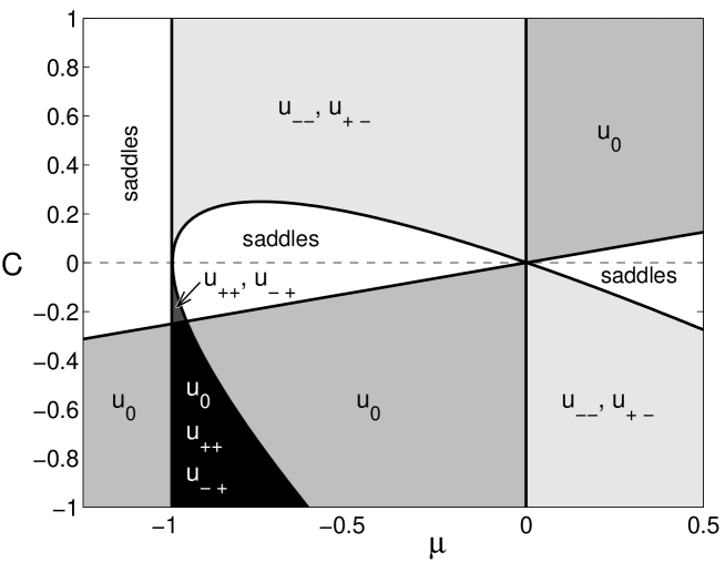
Figure 1: Stability diagram for the fixed points (FPs) of the two-dimensional map (6). In non shaded areas all the FPs are saddles. Shaded areas represent regions where the indicated FPs are centers. The diagonal line and the tilted parabola correspond, respectively, to $C=\mu/4$ and $(C+1+\mu)^{2}=1+\mu$.

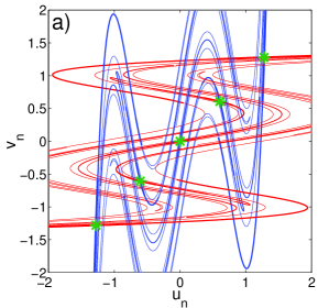
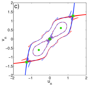
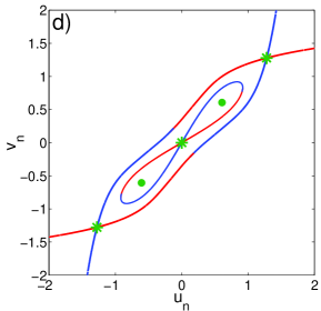
Figure 2: Homoclinic tangles generating localized solutions of Eq. (1) for $\mu=-0.6$, with the coupling constant $C$ increasing from left to right and from top to bottom: (a) $C=0.15$, (b) $C=0.4$, (c) $C=0.8$, and (d) $C=2$. Saddle points and centers are designated by asterisks and circles, respectively. For small $C$, the homoclinic intersections have a much richer structure, including homoclinic and heteroclinic connections between all five fixed points. For large $C$, only one homoclinic and one heteroclinic solutions survive (together with their $u_{n}\leftrightarrow-u_{n}$ symmetric counterparts).

We aim to look for a soliton solution with a frequency $\mu$ by substituting

$$\psi_{n}=u_{n}\exp(-i\mu t)$$ (4)

in Eq. (1). The real stationary lattice field $u_{n}$ must solve the equation

$$\mu u_{n}+C(u_{n+1}+u_{n-1}-2u_{n})+2u_{n}^{3}-u_{n}^{5}=0,$$ (5)

supplemented by the condition of vanishing of $u_{n}$ at $n\rightarrow\pm\infty$, i.e., the soliton can be looked for as a homoclinic solution of Eq. (5) (an alternative approach would be to use an algebraic method of Ref. [27]). Note that stationary soliton solutions of Eq. (5) depend on two parameters, $\mu$ and $C$.

We will study soliton solutions and their stability by viewing Eq. (5) as a recurrence relation between consecutive amplitudes, that can be cast in the form of a two-dimensional map,

$$\left\{\begin{array}[]{rcl}u_{n+1}&=&\displaystyle au_{n}-v_{n}-2C^{-1}u_{n}^{3}+C^{-1}u_{n}^{5}\\[8.61108pt] v_{n+1}&=&u_{n},\end{array}\right.$$ (6)

where $a\equiv 2-\mu/C$. Constant solutions to Eq. (1) correspond to fixed points (FPs) of this map. There exists at most five FPs, that we arrange in increasing order and label as $u_{-+},u_{--},u_{0},u_{+-},u_{++}$, with $u_{0}=0$ and

$$u_{\pm\pm}=\displaystyle\pm\sqrt{1\pm\sqrt{1+\mu}}.$$ (7)

The stability of all the FPs within the framework of map (6) can be easily derived from the linearization of the map around these FPs, leading to the stability chart displayed in Fig. 1.

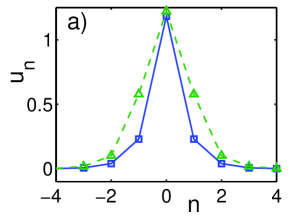
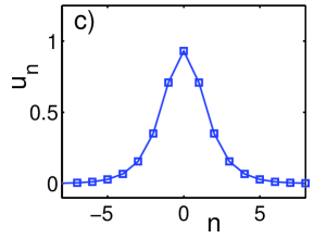
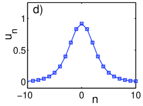
Figure 3: Typical examples of soliton solutions generated by the homoclinic tangles of Fig. 2 as the coupling parameter $C$ increases. Insets pertain to the same values of parameters as the corresponding insets in Fig. 2. (a) Pair of coexisting symmetric solution for small $C$. (b) As $C$ increases, only one stable symmetric solution exists (squares), together with a pair of asymmetric solutions (triangles and circles) appearing in small regions of the parameter space (the asymmetric solutions have been vertically displaced for clarity of presentation). (c) Further increase in $C$ destroys all stable solutions except for the symmetric one, that, as seen in panel (d), tends towards the continuum soliton in the limit of $C\rightarrow\infty$. The parameters are $\mu=-0.6$ and (a) $C=0.15$, (b) $C=0.4$, (c) $C=0.8$, (d) $C=2$.

In this framework, soliton solutions correspond to homoclinic orbits connecting the FP at origin ($u_{0}=0$) with itself, in the case when it is a saddle. The FP $u_{0}=0$ is a saddle for $\{\mu<0$ and $C>\mu/4\}$ and for $\{\mu>0$ and $C<\mu/4\}$. We are only interested in physically meaningful couplings so we restrict our attention to $C>0$. Furthermore, the regions for $\mu<-1$ and $\mu>0$ produce stable and unstable manifolds that do not intersect each other. Therefore, in the remaining of this work, we restrict our area of interest to $C>0$ with $-1<\mu<0$.

In Fig. 2, we depict a progression of the homoclinic tangles (webs of such orbits) emanating from the saddle points as the coupling constant $C$ increases. For small $C$, the homoclinic-connection structure is very rich, including many orbits (i.e., many soliton solutions). As $C$ increases, many connections disappear through a series of bifurcations (see below), so that a single homoclinic loop survives at very large $C$, which corresponds to the well-known exact soliton solution of the continuum CQ NLS equation [28].

Note that, in contrast with the cubic DNLS equation, the CQ discrete equation gives rise to a pair of extra fixed points that support heteroclinic orbits (as shown in Fig. 2). The detailed study of these heteroclinic orbits, which correspond to dark solitons or kinks, falls outside the scope of this work. Here we concentrate on the homoclinic orbits and (bright) soliton solutions corresponding to them.

In Fig. 3 we depict a selection of typical solitons corresponding to the homoclinic tangles in Fig. 2. Each solution is numerically generated by taking the soliton shape as predicted in an approximate form by the homoclinic intersections, and then applying a Newton-type algorithm to find a numerically exact localized solution of Eq. (5). In panel (a) we show a couple of solitons coexisting at given parameter values. Panel (b) depicts a triplet of coexisting solutions that form a part of a loop of pitchfork bifurcations responsible for the creation of asymmetric solutions (see below). Finally, panels (c) and (d) show the unique site-centered (the maximum of the soliton is located at a single central site, cf. Fig. 5(a)) solution which survives in the continuum limit, $C\rightarrow\infty$.

3 Multistability of discrete solitons

We now aim to explore the structure of the homoclinic tangles and their bifurcations in detail, varying the parameters $\mu$ and $C$. As previously mentioned, for small $C$ the rich homoclinic structure leads to the coexistence of multiple solitons at the same values of $\mu$ and $C$, which is a distinctive feature of the CQ model with the competing nonlinearities: in the cubic DNLS equations, this variety of solitons is not observed [1]. Principal types of the localized solutions for small $C$ (taking $C=0.1$ as an example) are depicted in Fig. 4. The following scheme is adopted to denote different species of the solitons. The solution generated by the first (main) homoclinic crossing of the stable and unstable manifolds of the origin (see Fig. 4(a)) is denoted by $S_{1}$. This family corresponds to site-centered solitons, the label $S$ standing for short, as the solitons of this type correspond to the shortest family of homoclinic crossings. As $C$ is increased, the $S_{1}$ soliton suffers a series of alternating stability switches (bifurcations). We use the notation $S_{k}$ to denote solitons corresponding to the series of stable regions between the stability switches. In this work we do not consider higher-order crossings corresponding to repeated iterates in both the stable and unstable manifolds, that would produce bound states of the discrete solitons, alias multi-humped or multibreather (non fundamental) solutions [29].

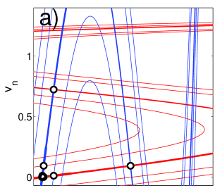
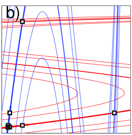
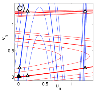
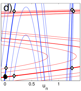
Figure 4: Multistability of discrete solitons in the CQ DNLS equation is illustrated by displaying the homoclinic tangles generating stable localized solutions (see Fig. 5). Parameters are $\mu=-0.6$ and $C=0.1$ (which corresponds to the point marked by the asterisk in the $T_{1}$ region in Fig. 6). Panels (a), (b), (c) and (d) correspond, respectively, to the discrete solitons of the $S_{1}$, $T_{1}$, $T_{2}$, and $T_{3}$ types (see definitions in the text).

The solitons generated by the homoclinic crossings in Figs. 4(b)-(d) correspond, in our notation, to $T_{1}$, $T_{2}$ and $T_{3}$ solitons, $T$ standing for tall solitons. They are generated by the second family of crossings, and are characterized by a higher soliton maximum, in comparison with their $S$ counterparts.

The subscript in the notation for the $T_{k}$ and $S_{k}$ solutions also helps to differentiate between site-centered solutions, for $k$ odd, and bond-centered (alias intersite-centered) ones for even $k$, which feature two central sites with equal magnitude, see examples in Fig. 5.

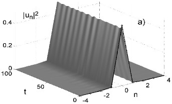
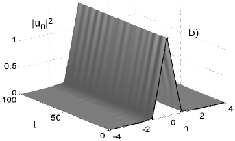
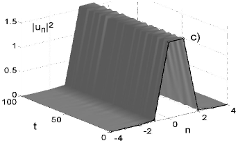
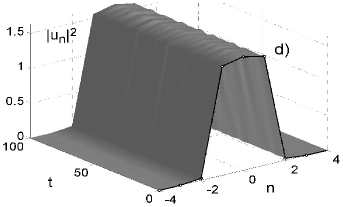
Figure 5: Evolution of the solitons generated by the homoclinic intersections depicted in Fig. 4 after adding random perturbations, with a relative amplitude of $5\%$, to the initial configuration (dark line).

The $S_{1}$, $T_{1}$, $T_{2}$ and $T_{3}$ solitons generated by the highlighted crossings in Fig. 4 are all stable solutions. The stability was checked by calculating the respective eigenvalues from Eq. (1) linearized around the stationary solutions, and also verified by direct numerical integration of the full equation (1) after adding a random perturbation to the soliton, with a (rather large) relative amplitude of $5\%$. The evolution of the so perturbed solutions is displayed in Fig. 5, where the unperturbed solitons are shown by dark lines for $t=0$. The perturbed solutions oscillates about the unperturbed solitons, confirming their stability (the oscillations do not fade because the system is conservative).

In order to identify a stability region of the soliton family in the $(\mu,C)$ parameter plane, we start with a particular soliton solution of the $S$ or $T$ type, generated as described above, and then continued it by varying the parameters, simultaneously computing the stability eigenvalues. The continuation procedure started at small $C$ where, as said above, it is easy to find a particular solution.

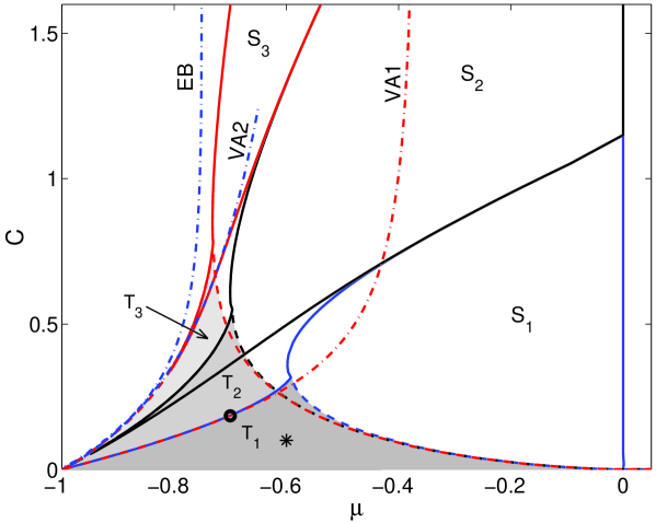
Figure 6: The stability diagram for single-hump localized solitons of the cubic-quintic discrete NLS equation (1). Note that each $S_{k}$ region has a “wedge” that penetrates into the corresponding $T_{k}$ region. The existence region of the solitons is bounded by the curve EB, at which the homoclinic connections of the origin disappear. The curves VA1 and VA2 show the variational approximations described in Section 5. A more detailed description is given in the text.

The resulting stability diagram for the solitons of the $S_{1,2,3}$ and $T_{1,2,3}$ types is displayed in Fig. 6. The $T_{k}$-stable regions (shaded in Fig. 6) feature a tent-like shape, with the base on the line $C=0$ with $-1\leq\mu\leq 0$. Since all these regions share the common base, there should be a nontrivial area where, presumably, the $T_{k}$ solitons exist and are stable for all values of $k$. It is also apparent from the stability diagram in Fig. 6 that the stability regions for the $S_{k}$ solutions with different $k$, in contrast to their $T_{k}$ counterparts, do not intersect each other. Therefore, the solitons of the $S$ type feature no multistability.

We note that each $S_{k}$ stability region features a wedge that penetrates into the region of stability of the $T_{k}$ solitons. Particularly, the $T_{1}$ region is completely embedded in the $S_{1}$ region. This property tends to suggest that, for any $k$, there always exists non-empty regions where the $T_{k}$ and $S_{k}$ solitons coexist and are simultaneously stable. It is interesting too that the $S$-stability regions outlive their $T$-counterparts as $C$ increases. This is due to the fact that the $T$ solutions correspond to the second family of homoclinic crossings that disappear, in saddle-node bifurcations (see below), earlier than the first family of the crossings (i.e., the $S$ solutions).

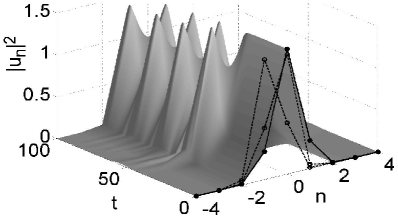
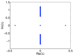
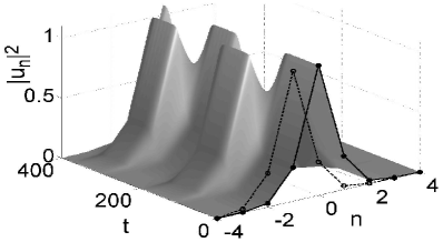
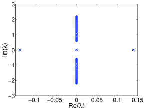
Figure 7: Evolution of unstable solitons (left panels), together with their instability spectrum (right panels). The top row depicts the evolution of an unstable $S_{2}$ soliton, shown by the dashed line in Fig. 3(a) for $(\mu,C)=(-0.6,0.15)$, initiated by a small perturbation. After some transient, the initial configuration (solid line) is changed by one featuring oscillations between two asymmetric states (dashed lines). The bottom row depicts the evolution of an unstable symmetric $S_{1}$ solution from Fig. 3(b) for $(\mu,C)=(-0.6,0.4)$. The evolution amounts to oscillations between the initial configuration (solid line) and its translation by one site (dashed line). The respective (in)stability spectra for the two solutions in the left column are depicted in the right column.

Existence regions for the solitons, which may be broader than the regions where the solitons are stable, are defined as those in which the stable and unstable manifolds emanating from the origin do intersect. We have computed such a region numerically. In Fig. 6, it is located to the right of the dashed-dotted line EB (existence boundary). To the left of this curve, no localized solutions are possible. As $C$ increases, the EB curve approaches the line $\mu=-3/4$, that corresponds to the existence border for solitons in the continuum limit of the CQ equation [16]. More specifically, the existence regions of the $T$ solutions exactly coincide with their stability regions, i.e., the solitons of the $T$ type are always stable. The existence region for the $S$ solutions has a complex structure, contained in the region where homoclinic connections exists to the right of the EB curve, while the stability area for these solitons is really smaller than the existence region. We also note that (as explained in detail below) the $S_{k}$ solutions represent only two distinct families of solitons, one site-centered (for odd $k$) and one bond-centered (for even $k$).

Since some solitons of the $S$ type are unstable, it is necessary to determine what the instability transforms them into. As an example, in the top row of Fig. 7 we display the evolution of an unstable $S_{2}$ soliton in the stability region of $T_{1}$ (for $(\mu,C)=(-0.6,0.15)$, see asterisk in Fig. 6), together with its instability eigenvalues. The nonlinear evolution proceeds through periodic oscillations between two asymmetric states (see dashed lines for $t=0$).

In the bottom row of Fig. 7 we show the evolution of another unstable solution and its associated instability spectrum. In this case, we take the $S_{1}$ solution at $(\mu,C)=(-0.6,0.4)$, which is in the gap between the stability regions of the $S_{1}$ and $S_{2}$ solutions. A loop of pitchfork bifurcations occurs in the gaps between consecutive $S$-stability regions, see details in the next section. The evolution of this unstable solution amounts to periodic oscillations between the original $S_{1}$ soliton (the solid line at $t=0$) and its translation by one site (the dashed line at $t=0$)). Therefore, this solution is a time-periodic one, being close to a heteroclinic connection linking the two unstable solutions, $S_{1}$ and its translation.

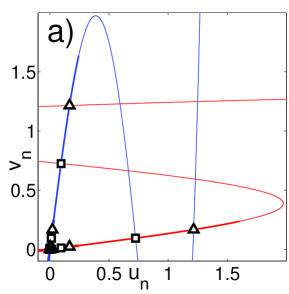
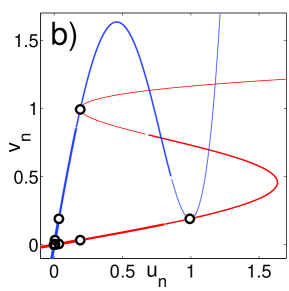
Figure 8: Homoclinic tangles generating the solitons in Fig. 11. a) the point $(\mu,C)=(-0.6,0.1)$ belongs to the bistability region (see asterisk in Fig. 6) that generates two solitons (triangles, $T_{1}$, and squares, $S_{1}$). b) the point $(\mu,C)=(-0.7,0.1855)$ is located at the bifurcation curve (see the circle in Fig. 6), hence the two solutions collapse into one (see the right panel in Fig. 11).

4 Bifurcations of the discrete solitons

In this section we aim to explain how the $T_{1}$ solutions disappear and how the evolution of the $S$ solutions leads to stability changes and creation of pairs of stable asymmetric solitons. It is straightforward to understand the simultaneous disappearance of the $S$ and $T$-type solutions as $C$ increases. The boundary on which this happens corresponds to the left side of the tent-like stability area of the $T$ solutions in Fig. 6. The $S_{k}$ and $T_{k}$ solutions collide on this boundary and disappear in a saddle-node bifurcation. This bifurcation can be easily followed using the homoclinic-tangle approach (see Fig. 8). Before the bifurcation occurs, i.e., below the boundary (see the asterisk in Fig. 6), two intersections, identified by squares and triangles in Fig. 8(a), generate the solitons of the types $S_{1}$ and $T_{1}$, respectively, which are are shown in the left panels of Fig. 11. In contrast, when the bifurcation curve is approached, see Fig. 8(b), the stable and unstable manifolds barely intersect, and the two solitons are nearly identical. Exactly at the bifurcation, the manifolds touch tangentially, and only one solution is generated (i.e., the $S_{1}$ and $T_{1}$ solitons are identical at this point). After this saddle-node bifurcation, these solutions do not exist anymore.

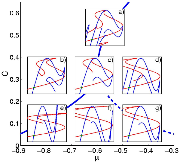
Figure 9: Different types of bifurcations around the cusp of the $T_{1}$ region. A saddle-node bifurcation corresponding to panel (e) annihilates the pair of the $S_{1}$ and $T_{1}$ solutions (the same bifurcation was depicted in Fig. 8). Another saddle-node bifurcation corresponds to panel (g) and is responsible for the destruction of the $T_{1}$ solution. Going from (d) to (a), there is a pitchfork bifurcation which is responsible for the loss of stability of the symmetric soliton and the creation of a pair of stable asymmetric ones (see further details in Fig. 10).

Another family of noteworthy bifurcations points corresponds to cuspidal points of the $T$-stability regions. Three types of bifurcations occur near these points: (A) the saddle-node bifurcation described above, at which the $S$ and $T$ solitons collide and disappear; (B) another saddle-node bifurcation, at which the $T$ solutions disappear; and (C) a bifurcation at which the $S$ solitons lose their stability. These bifurcations are depicted in Fig. 9 as follows: (A) corresponds to going through panels (f)$\rightarrow$(e)$\rightarrow$(b), (B) is displayed by a chain of panels (f)$\rightarrow$(g)$\rightarrow$(d), and (C) corresponds to going through (d)$\rightarrow$(a)$\rightarrow$(b).

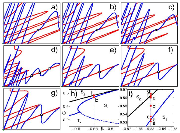
Figure 10: The pitchfork bifurcation leading to asymmetric soliton solutions. This series of plots was obtained by keeping $\mu=-0.55$ and varying $C$ from the $S_{1}$ to $S_{2}$ regions, as shown in insets (h) and (i). The series includes the following panels: (a) the $S_{1}$ region before the bifurcation; (b) at the pitchfork bifurcation; (c), (d) and (e) in the region where asymmetric solitons exist; (f) is a reverse pitchfork that destroys the asymmetric solutions; and (g) the $S_{2}$ region after the latter bifurcation. The square dot represents the same homoclinic orbit throughout the bifurcation, while the triangle and circle in (d) correspond to the asymmetric solitons from Fig. 3.

Bifurcation (C) deserves more attention. In Fig. 10 we depict in more detail the bifurcation scenario corresponding to a route from the stability region of $S_{1}$ to its $S_{2}$ counterpart, which passes through a gap where no $S$ solution is stable. Panels (a) through (g) show the homoclinic tangles as $C$ increases, for fixed $\mu=-0.55$. Parameter values for each of these panels are indicated in panel (h) and its magnification, panel (i). From this figure, the existence of a pitchfork loop —a supercritical pitchfork shortly followed by a reverse subcritical one— is evident. In panel (a) we depict by a square point one of the homoclinic intersections, which gives rise to solution $S_{1}$. As $C$ increases, the supercritical pitchfork bifurcation is reached, panel (b), that gives rise to a pair of extra homoclinic intersections (see panel (c) and triangle and circle in panel (d)). As $C$ increases further, the reverse subcritical pitchfork occurs, eliminating the extra pair of intersections.

Quite interesting are the shape and stability of solitons that this extra pair generates in the narrow gap between the $S_{k}$ and $S_{k+1}$ stability regions (which coincides with the region of the pitchfork loop), where these new solutions exist. They represent asymmetric solitons of the CQ DNLS equation, which are depicted in Fig. 3(b) by means of triangles and circles. As might be expected, the stability is swapped by the pitchfork bifurcations. Indeed, the stable $S$ solitons are unstable inside the pitchfork loop, where the new asymmetric solutions are stable. An example of unstable evolution of an $S$ soliton inside the pitchfork loop is shown in the bottom row of Fig. 7. We stress that such pitchfork loops, and the respective asymmetric solitons, do not exist in the cubic DNLS equation (asymmetric solitons were also found in a DNLS equation with a mixture of cubic onsite and intersite nonlinearities [19]).

Further inspection of the pitchfork loop demonstrates that, if the $S_{1}$ site-centered soliton looses its stability through the direct bifurcation, then the reverse bifurcation, which closes the loop, stabilizes an $S_{2}$ bond-centered soliton. At the next pitchfork loop (in the gap between stability of $S_{2}$ and $S_{3}$), the latter bond-centered solution gets destabilized and, after the loop, an $S_{3}$ site-centered soliton gains its stability. As $C$ is increased further, this process repeats itself, creating stability bands for the $S_{k}$ solitons for larger $k$. In fact, all the solutions $S_{k}$ represent only two distinct soliton families emanating from the principal homoclinic intersection: of site-centered solutions, and of bond-centered ones, the pitchfork loops conducting stability swaps between the two families. For given $S_{k}$, the number of the pitchfork loops passed by the soliton, while developing from the anti-continuum ($C=0$) limit, is $k-1$.

The existence of stable bond-centered solitons is a noteworthy feature by itself, as in the usual DNLS model with the cubic nonlinearity only site-centered states are stable (in the DNLS equation with the saturable onsite nonlinearity, stable bond-centered solitons were found too [20]). An interesting issue which still has to be addressed is whether there exists an accumulation curve for the pitchfork loops, or the loops continue to appear as one approaches the continuum limit, $C=\infty$.

5 The variational approximation

The variational approximation (VA) can be used to describe the shape of stationary soliton solutions in an analytical form. The method will not only be successful in approximating the shape of the most fundamental solitons, but will also predict the saddle-node bifurcation where the $T_{1}$ and $S_{1}$ solutions collide and disappear.

The only tractable ansatz for the VA in the discrete models is one based on an exponential cusp, that was applied in Ref. [25] to solitons in the above-mentioned DNLS equation with an arbitrary power nonlinearity :

$$u_{n}=Ae^{-\alpha|n|},$$ (8)

with real positive constants $A$ and $\alpha$. We identify the value of $\alpha$ without the resort to the VA proper, but rather from the substitution of ansatz (8) in Eq. (5) linearized for the decaying tail of the soliton, which yields

$$\alpha=\ln\left(\frac{a}{2}+\sqrt{\left(\frac{a}{2}\right)^{2}-1}\right)$$ (9)

(recall $a\equiv 2-\mu/C$). Thus, a necessary (but not sufficient) condition for the existence of any soliton solution is $a>2$, or $\mu<0$ (since we set $C>0$, it will then guarantee that Eq. (9) yields a real positive $\alpha$). We stress that the latter soliton-existence condition is an exact one, as it follows from the straightforward consideration of the exponentially localized tails of the soliton, and does not exploit any approximation.

Now we invoke the VA proper, treating the amplitude $A$ in ansatz (8) as a variational parameter, while $\alpha$ was already fixed as per Eq. (9) (i.e., by the condition that the ansatz must match the correct asymptotic form of the soliton solution).

Figure 11: Soliton solutions of Eq. (5) for $(\mu,C)=(-0.6,0.1)$ (left) and $(\mu,C)=(-0.7,0.1845)$ (right) are shown on straight (top) and logarithmic (bottom) scales. Points and lines correspond, respectively, to numerically exact solutions and ones predicted by the variational approximation. The right panels correspond to a point $(\mu,C)$ close to the collision of the soliton solutions of the $S_{1}$ and $T_{1}$ types (see the circle in Fig. 6).

The stationary equation (5) can be derived from the Lagrangian

$${L}=\displaystyle\sum_{n=-\infty}^{\infty}\left[\mu u_{n}^{2}+\frac{B}{2}u_{n}^{4}-\frac{Q}{3}u_{n}^{6}-C(u_{n+1}-u_{n})^{2}\right].$$ (10)

The substitution of the ansatz into the Lagrangian and explicit calculation of the sum lead to the following effective Lagrangian, which is the main ingredient of the VA [30]:

$${L}_{\mathrm{eff}}{(A)}=\displaystyle\mu A^{2}\coth(\alpha)+A^{4}\coth(2\alpha)-\frac{A^{6}}{3}\coth(3\alpha)-2\tanh(\alpha/2)CA^{2}.$$ (11)

Then, the Euler-Lagrange equation, $d{L}_{\mathrm{eff}}{(A)/dA=0}$, yields a quadratic equation for $A^{2}$,

$$-\coth(3\alpha)\left(A^{2}\right)^{2}+2\coth(2\alpha)\left(A^{2}\right)+\mu\coth(\alpha)-2\tanh(\alpha/2)C=0.$$ (12)

  

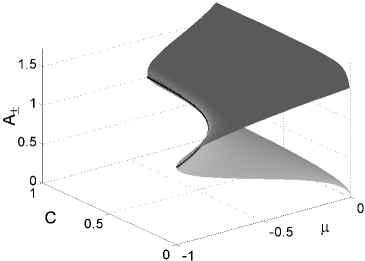
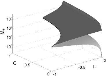
Figure 12: Amplitude $A$ (left) and norm $M$ (right) for the two soliton solutions predicted by the VA (the scale for the norm is logarithmic). The top and bottom branches correspond to the tall and short solitons, respectively. The dark solid line represent the bifurcation curve where the two solutions are predicted to coalesce and disappear.

Equation (12) indicates that there may be two different solutions. The top panel of Fig. 12 depicts the amplitude associated with these two solutions predicted by the VA. It is clear that the two solutions coalesce and disappear at the bifurcation curve (solid line). In Fig. 11 we display examples of these two variational solutions, together with the ones obtained numerically from Eq. (5) through Newton iterations. It is observed that the match between the numerical and variational solutions is extremely good for small values of the coupling parameter $C$. For larger values of $C$, the solution tends to its continuum (smooth) analogue where the cusp-shaped ansatz (8) is obviously irrelevant.

The VA predicts the bistable solutions of the type (8) inside the $(\mu,C)$-parameter regions where the quadratic equation (12) admits two distinct positive roots. The comparison with numerical results in Fig. 11 immediately shows that the two different variational solutions exactly correspond to the $S_{1}$ and $T_{1}$ solitons, as they were defined above. Therefore, the curve where Eq. (12) has a double root represents the saddle-node collision of $S_{1}$ and $T_{1}$. This bifurcation curve predicted by the VA is depicted by the dashed-dotted curve labeled VA1 in Fig. 6. It is quite remarkable that the approximation based on the simple ansatz (8) is able to capture the saddle-node bifurcation so well for small $C$.

It is possible to refine the VA approach by allowing a more general ansatz of the form

$$u_{n}=\left\{\begin{array}[]{lcl}\phantom{\beta}Ae^{-\alpha|n|}&\mathrm{~{}if~{}}&|n|>0,\\[2.15277pt] \beta A&\mathrm{~{}if~{}}&n=0,\end{array}\right.$$ (13)

where we introduce a new free parameter $\beta$. This new ansatz is able to predict the existence of the solitons of two distinct types, which can me immediately identified with short ($S$) and tall ($T$) solitons, that were described in detail above.

The new variational ansatz (13), with two independent variational parameters $(A,\beta)$, is able to very accurately predict the whole existence region of the $T_{1}$ solution, as well as the saddle-node bifurcation which creates the $S_{3}$ solution. The boundary of the $S_{3}$ solitons predicted by the improved VA is depicted by the dash-dotted line VA2 in Fig. 6. As seen from the figure, the new VA gives an extremely good approximation for the boundary, up to $C\lesssim 1$. The results for the existence region of the $T_{1}$ soliton predicted by this VA are not depicted in Fig. 6 because they exactly coincide (up to the resolution of the figure) with both, left and right, numerically found boundaries for the $T_{1}$ soliton, see the darker shaded area in Fig. 6 (the simple VA, based on ansatz (8), which gives rise to curve VA1, only captured the left boundary).

The improved VA with ansatz (13) is also able to pick up solutions with a dip at the central site, corresponding to $\beta<e^{-\alpha}$ in the ansatz, i.e., a bound state of two solitons, or multibreather [29]). Thus, the modified VA is able to describe the respective bifurcation curves too (results not presented here).

A well-known approach to predicting the stability for soliton families is based on the Vakhitov-Kolokolov (VK) criterion [31]. The VK criterion states that a solution family, parameterized by the frequency $\mu$, as in Eq. (4), may be stable if $dM/d\mu<0$, and is definitely unstable otherwise, where $M$ is the soliton’s norm defined as per Eq. (3). The simplest variational ansatz (8) yields $M=A^{2}\coth(\alpha)$ [note that both $\alpha$ and $A$ depend on $(\mu,C)$ through Eqs. (9) and (12)]. The norm given by the latter expression is depicted, as a function of $(\mu,C)$, in the right panel of Fig. 12. It is clear from the figure that $dM/d\mu>0$ for the $T_{1}$ soliton, and $dM/d\mu<0$ for $S_{1}$ (these results can be proven analytically, within the framework of the VA). Thus, the VK criterion suggests that the $T_{1}$ soliton is unstable, while its $S_{1}$ counterpart may be stable. Comparing this conclusion with the numerical results for the stability reported above we conclude that the VK criterion does not apply to our model. In fact, similar conclusions for the failure of the VK criterion where obtained in the continuous CQ NLS equation with an external potential, that might be both a single rectangular potential well [17], and a periodic lattice of rectangular wells (the above-mentioned Kronig-Penney potential) [16].

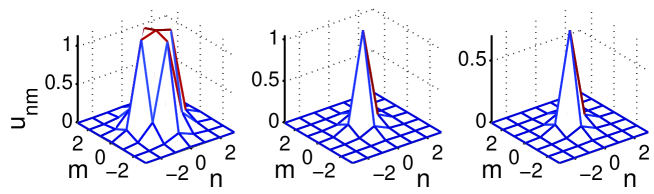
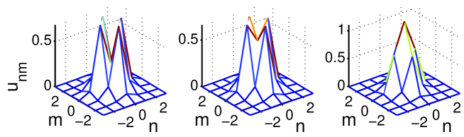
Figure 13: Two-dimensional coexisting soliton solutions for $(\mu,C)=(-0.6,0.07)$. The top row depicts three coexisting stable soliton solutions while the bottom row represents three coexisting unstable soliton solutions. All these solutions were obtained by Newton iteration on the steady state equation with initial seeds predicted by the two-dimensional variational approximation with ansatz (14).

A natural question that arises is the existence of multistable solutions in higher dimensional lattices. The higher dimensional equivalent of (1) is obtained by replacing the one-dimensional index $n$ and the discrete Laplacian by their higher-dimensional analogues. Unfortunately, the homoclinic approach is not applicable in higher dimensional lattices. Nonetheless, the variational approach presented here is still amenable in the higher dimensional case. Namely, a natural ansatz equivalent to (13) but now in two dimensions (2D) becomes

$$u_{nm}=\left\{\begin{array}[]{lcl}\phantom{\beta}Ae^{-\alpha(|n|+|m|)}&\mathrm{~{}if~{}}&|n|+|m|>0,\\[2.15277pt] \beta A&\mathrm{~{}if~{}}&n=m=0,\end{array}\right.$$ (14)

where now we have two indexes $(m,n)$ along the two spatial dimensions, and the decay $\alpha$ is the same as for the one-dimensional case [cf. Eq. (9)]. Preliminary results indicate the coexistence of stable soliton solutions in the 2D model. As an example we depict in Fig. 13 six coexisting solutions for the same parameter values. The top row in the figure depicts three stable coexisting solutions. It is worth mentioning that the variational approach for the 2D case is also able to capture other solutions such as, stable and unstable, multi-humped profiles (see bottom row of Fig. 13). A detailed stability analysis for higher dimensional (2D and 3D) soliton solutions falls outside of the scope of the present manuscript and will be presented elsewhere.

6 Conclusions and extensions

The objective of this work was to introduce the discrete nonlinear Schrödinger (DNLS) equation with the competing cubic-quintic (CQ) nonlinearities. Besides being a new dynamical model, this model may also apply to the description of an array of optical waveguides with the intrinsic CQ nonlinearity.

We have studied the multistability of discrete solitons in the model, looking for homoclinic solutions to the respective stationary discrete equation. Regions of the existence and stability of single-humped soliton solutions were identified by using a numerical continuation method based on Newton-type iterations. The stability of the various types of the solitons was investigated through numerical evaluation of eigenvalues for small perturbations. The resulting stability diagram suggests the existence of an infinite family of branches of stable solitons of the aforementioned type $T_{k}$, for sufficiently small values of the coupling constant $C$. As $C$ increases, these solutions get destroyed through saddle-node bifurcations. We have also identified another type of discrete soliton solutions, $S_{k}$, with $S_{1}$ surviving in the continuum limit, $C\rightarrow\infty$. The stability of solutions of the latter type ($S$) changes, with the increase of $C$, through a series of small pitchfork loops (each opens with a supercritical pitchfork, which is shortly followed by a reverse supercritical one). Inside the loops the symmetric solitons $S_{k}$ loose their stability, while a pair of stable asymmetric solutions is created. The latter solutions have no counterpart in the cubic DNLS equation, nor in the continuum CQ NLS equation. Finally, using the variational approximation (VA), we were able to approximate the main branches of the solutions and their bifurcations for small $C$. We have also proposed an improved version of the VA, with two free parameters rather than one, that drastically (qualitatively) upgrades the accuracy of the VA, making it possible to predict simultaneously the most fundamental solitons and some higher-order ones.

An interesting extension of this work would be to thoroughly investigate localized solutions in the two-dimensional version of the CQ DNLS equation, which may be realized, for instance, as a bunch of the corresponding nonlinear optical waveguides (cf. the recently reported experimental realization for linear waveguides [32]). In particular, the existence and stability of asymmetric solitons in the two-dimensional model would be an issue of great interest. Another promising direction for further considerations may be the study of kink solutions, corresponding to heteroclinic trajectories generated by the intersection of the stable and unstable manifolds of different fixed points of the map (6).

As concerns the underlying mathematical theory, an intriguing issue is to understand why the Vakhitov-Kolokolov criterion was found to consistently fail in the discrete CQ NLS equation and its counterpart with a periodic potential in the continuum case [16, 17].

References

- [1] P. G. Kevrekidis, K. Ø. Rasmussen, A. R. Bishop, Int. J. Mod. Phys. B 15 (2001) 2833.
- [2] D. N. Christodoulides, R. I. Joseph, Opt. Lett. 13 (1988) 794.
- [3] H. S. Eisenberg, Y. Silberberg, R. Morandotti, A. R. Boyd, J. S. Aitchison, Phys. Rev. Lett. 81 (1998) 3383.
- [4] D. N. Christodoulides, F. Lederer, Y. Silberberg, Nature 424 (2003) 817.
- [5] J. W. Fleischer, G. Bartal, O. Cohen, T. Schwartz, O. Manela, B. Freedman, M. Segev, H. Buljan, N. K. Efremidis, Opt. Exp. 13 (2005) 1780.
- [6] D. Cheskis, S. Bar-Ad, R. Morandotti, J. S. Aitchison, H. S. Eisenberg, Y. Silberberg, D. Ross, Phys. Rev. Lett. 91 (2003) 223901.
- [7] A. Trombettoni and A. Smerzi, Phys. Rev. Lett. 86 (2001) 2353; G. L. Alfimov, P. G. Kevrekidis, V. V. Konotop, M. Salerno, Phys. Rev. E 66 (2002) 046608; R. Carretero-González and K. Promislow, Phys. Rev. A 66 (2002) 033610.
- [8] F. S. Cataliotti, S. Burger, C. Fort, P. Maddaloni, F. Minardi, A. Trombettoni, A. Smerzi, M. Inguscio, Science 293 (2001) 843; M. Greiner, O. Mandel, T. Esslinger, T. W. Hänsch, I. Bloch, Nature 415 (2002) 39.
- [9] M. A. Porter, R. Carretero-Gonzalez, P. G. Kevrekidis, B. A. Malomed, Chaos 15 (2005) 015115.
- [10] S. Aubry, Physica 103D (1997) 201; R. S. MacKay and S. Aubry. Nonlinearity 7 (1994) 1623; S. Flach and C. R. Willis, Phys. Rep. 295 (1998) 181; G. P. Tsironis, Chaos 13 (2003) 657.
- [11] D. K. Campbell, S. Flach, Y. S. Kivshar, Physics Today 57 (2004) 43.
- [12] M. Sato, B. E. Hubbard, A. J. Sievers, B. Ilic, D. A. Czaplewski, H. G. Craighead, Phys. Rev. Lett. 90 (2003) 044102; M. Sato and A. J. Sievers, Nature 432 (2004) 486.
- [13] R. Carretero-González, P. G. Kevrekidis, B. A. Malomed, D. J. Frantzeskakis. Phys. Rev. Lett. 94 (2005) 203901; P. G. Kevrekidis, B.A. Malomed, D. J. Frantzeskakis, R. Carretero-González. Phys. Rev. Lett. 93 (2004) 080403.
- [14] T. Dauxois and M. Peyrard. Physics of Solitons, Cambridge University Press (2005).
- [15] F. Smektala, C. Quemard, V. Couderc, A. Barthélémy, J. Non-Cryst. Solids 274 (2000) 232; G. Boudebs, S. Cherukulappurath, H. Leblond, J. Troles, F. Smektala, F. Sanchez, Opt. Commun. 219 (2003) 427; C. Zhan, D. Zhang, D. Zhu, D. Wang, Y. Li, D. Li, Z. Lu, L. Zhao, Y. Nie, J. Opt. Soc. Am. B 19 (2002) 369.
- [16] I. M. Merhasin, B. V. Gisin, R. Driben, B. A. Malomed, Phys. Rev. E 71 (2005) 016613; J. Wang, F. Ye, L. Dong, T. Cai, Y.-P. Li, Phys. Lett. A 339 (2005) 74.
- [17] B. V. Gisin, R. Driben, B. A. Malomed, J. Opt. B: Quant. Semiclass. Opt. 6 (2004) S259.
- [18] W. D. Li and A. Smerzi, Phys. Rev E 70 (2004) 016605; B. T. Seaman, L. D. Carr, M. J. Holland, Phys. Rev. A 71 (2005) 033622.
- [19] M. Öster, M. Johansson, and A. Eriksson Phys. Rev. E 67 (2003) 056606.
- [20] M. Stepić, D. Kip, L. Hadžievski, A. Maluckov, Phys. Rev E 69 (2004) 066618; L. Hadžievski, A. Maluckov, M. Stepić, D. Kip, Phys. Rev. Lett. 93 (2004) 033901.
- [21] A. Khare, K.Ø. Rasmussen, M. R. Samuelsen, A. Saxena, J. Phys. A Math. Gen. 38 (2005) 807.
- [22] V. O. Vinetskii and N. V. Kukhtarev, Sov. Phys. Solid State 16 (1975) 2414.
- [23] F. Chen, M. Stepic, C. E. Ruter, D. Runde, D. Kip, V. Shandarov, O. Manela, M. Segev, Opt. Exp. 13 (2005) 4314.
- [24] E. W. Laedke, K. H. Spatschek, S. K. Turitsyn, Phys. Rev. Lett. 73 (1994) 1055; S. Flach, K. Kladko, R. S. MacKay, Phys. Rev. Lett. 78 (1997) 1207.
- [25] B. A. Malomed and M. I. Weinstein, Phys. Lett. A 220 (1996) 91.
- [26] J. Dorignac, J. C. Eilbeck, M. Salerno, A. C. Scott, Phys. Rev. Lett. 93 (2004) 025504.
- [27] G. P. Tsironis, J. Phys. A: Math. Gen. 35 (2002) 951.
- [28] Kh. I. Pushkarov, D. I. Pushkarov, I. V. Tomov, Opt. Quant. Electr. 11 (1979) 471; S. Cowan, R. H. Enns, S. S. Rangnekar, S. S. Sanghera, Can. J. Phys. 64 (1986) 311.
- [29] T. Bountis, H. W. Capel, M. Kollmann, J. C. Ross, J. M. Bergamin, J.P. van der Weele, Phys. Lett. A 268 (2000) 50; T. Kapitula, P. G. Kevrekidis, B. A. Malomed, Phys. Rev. E 63 (2001) 036604; V. Koukouloyannis and S. Ichtiaroglou, Phys. Rev. E 66 (2002) 066602; V. Koukouloyannis, Phys. Rev. E 69 (2004) 046613.
- [30] B. A. Malomed, Progr. Opt. 43 (2002) 71.
- [31] N. G. Vakhitov and A. A. Kolokolov, Izv. Vyssh. Uchebn. Zaved. Radiofiz. 16 (1973) 10120 [Radiophys. Quantum Electron. 16 (1973) 783].
- [32] T. Pertsch, U. Peschel, F. Lederer, J. Burghoff, M. Will, S. Nolte, A. Tunnermann, Opt. Lett. 29 (2004) 468.