Dynamic Critical approach to Self-Organized Criticality.

Abstract

A dynamic scaling Ansatz for the approach to the Self-Organized Critical (SOC) regime is proposed and tested by means of extensive simulations applied to the Bak-Sneppen model (BS), which exhibits robust SOC behavior. Considering the short-time scaling behavior of the density of sites ($\rho(t)$) below the critical value, it is shown that i) starting the dynamics with configurations such that $\rho(t=0)\rightarrow 0$ one observes an initial increase of the density with exponent $\theta=0.12(2)$; ii) using initial configurations with $\rho(t=0)\rightarrow 1$, the density decays with exponent $\delta=0.47(2)$. It is also shown that he temporal autocorrelation decays with exponent $C_{a}=0.35(2)$. Using these, dynamically determined, critical exponents and suitable scaling relationships, all known exponents of the BS model can be obtained, e.g. the dynamical exponent $z=2.10(5)$, the mass dimension exponent $D=2.42(5)$, and the exponent of all returns of the activity $\tau_{ALL}=0.39(2)$, in excellent agreement with values already accepted and obtained within the SOC regime.

Nearly two decades ago, Bak et al. pb proposed the celebrated concept of Self-Organized Criticality (SOC) in order to describe complex systems capable of evolving toward a critical state without the need of tuning any control parameter. This is in contrast to the case of standard critical behavior where critical points are reached by tuning a suitable control parameter (temperature, pressure, etc.). The study of SOC behavior has attracted huge attention due to its ubiquity in a great variety of systems in the fields of biology (evolutionary models), geology (earthquakes), physics (flick noise), zoology (prey-predators and herds), chemistry (chemical reactions), social sciences (collective behavior of individuals), ecology (forest-fire), neurology (neural networks), etc. book1 ; book2 .

In spite of the considerable effort invested in the study of SOC, it is surprising that little attention has been drawn to the understanding of the dynamic approach to the SOC regime when a system starts far from it. This issue is relevant for a comprehensive description of the phenomena since the SOC state behaves as an attractor of the dynamics. For the case of standard criticality, the existence of a short-time universal dynamic scaling form for model A has only recently been established. In fact, according to a field-theoretical analysis followed by an $\epsilon-$expansion Schmittman , which was subsequently been extensively confirmed by means of numerical simulations Huse , a short-time universal dynamic evolution that sets in right after a time scale $t_{mic}$, which is large enough in the microscopic sense but still very small in the macroscopic one, has been identified. It is worth mentioning that by means of short-time measurement one can not only evaluate the dynamic exponent $z$ and relevant (static) exponents, but also the exponent ($\theta$) describing the scaling behavior of the initial increase of the order parameter of model A.

Within this context, the aim of this work is to propose a dynamic scaling Ansatz to describe the approach to the SOC state. Furthermore, our proposal is validated by extensive simulations of the evolutionary Bak-Sneppen model, showing that the dynamic approach to the SOC state is in fact critical and its study allows us to evaluate exponents that are in excellent agreement with independent measurements performed within the SOC regime.

The Bak-Sneppen (BS) model is aimed at simulating the evolution of life through individual mutations and their relation in the food chain bs ; bs2 ; bs3 ; paczuski . Each site of a $d-$dimensional array of side $L$ represents a species whose fitness is given by a random number $f$ taken from a uniform distribution $P(f)$ in the range $[0,1]$. The system evolves according to the following rules: (1) The site with the smallest fitness is chosen. (2) A new fitness is assigned to that site, i.e., a random number taken from $P$. This rule is based on the Darwinian survival principle, i.e., the species with less fitness are replaced or mutated. (3) At the same time, the fitness of the nearest-neighbor sites are changed. This rule simulates the impact of the mutation over the environment.

The BS model is the archetype example of extremal dynamics and perhaps, it is the simplest example of a system exhibiting a robust SOC behavior. We will perform simulations in $d=1$, assuming periodic boundary conditions. It is well known that the system reaches a stationary (SOC) state where the density $\rho$ of sites with fitness below a critical value is negligible ($f<f_{c}$, with $f_{c}=0.66702(3)$), but it is uniform above $f_{c}$ paczuski . Within the SOC state, the BS model exhibits scale-free evolutionary avalanches and punctuated equilibrium bs ; paczuski .

The dynamic scaling Ansatz. The short-time dynamic scaling form has originally been formulated for the Ising model with two state spins Huse . In the absence of magnetic fields, the Ising magnet exhibits a second-order phase transition when the temperature is tuned at the critical point (i.e., standard critical behavior). By analogy, we also considered that in the BS model, each site can only be in one of two possible states $\sigma_{i}$: occupied ($\sigma_{i}=1$) when its fitness is below $f_{c}$ or empty ($\sigma_{i}=0$) when its fitness is above $f_{c}$. Furthermore, since the magnetization goes to zero at the critical temperature of the Ising system, while in the BS model the density of sites $\rho$ also vanishes when the SOC regime is reached paczuski , it is also reasonable to propose a scaling Ansatz for the density. However, it is worth mentioning that the BS model lacks a control parameter, such as the temperature for the Ising model. Hence, in the limit $L\rightarrow\infty$, the proposed scaling reads

$$\rho(t,\rho_{0})=b^{-\aleph}\rho(b^{-z}t,b^{x_{0}}\rho_{0})$$ (1)

where $\rho_{0}$ is the initial density, $z$ is the dynamic exponent, $x_{0}$ is the exponent of the rescaling of $\rho_{0}$, $\aleph$ is an exponent, and $b$ is a scaling variable.

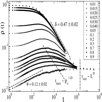
Figure 1: Temporal evolution of average density for several values of initial density $\rho_{0}$ as listed in the figure.

Simulation results and discussion. Computer simulations were performed in ensembles of $10^{3}$ different systems having the same initial density of sites with fitness below $f_{c}$. Notice that usually the site with the smallest fitness value at time $t$ is called the active site. Figure 1 shows the temporal evolution of density $\rho(t,\rho_{0})$ as obtained for different values of $\rho_{0}$. Three different regimes can be distinguished: i) A short-time regime $(0<t<t_{max}\approx 10^{3})$, which holds for low initial densities $\rho_{0}<0.1$, where the density exhibits an initial increase. Since the value of the “effective” exponent slightly depends on $\rho_{0}$, as ussually Huse , we have performed an extrapolation obtaining $\theta=0.12(2)$ in the $\rho_{0}\rightarrow 0$ limit. ii) An intermediate-time regime $(t_{max}<t<t_{stat}\approx 10^{6})$ where the density decreases also following a power-law with exponent $\delta=0.47(2)$, and iii) A long-time regime $(t_{stat}<t)$, where the system arrives at a stationary state with a constant average density $\rho_{stat}$.

In order to understand the observed behavior it is useful to analyze first a simulation started with a single site ($\rho_{0}=1/L$). One observes (not shown here for the sake of space) a single avalanche and the density increases monotonically with exponent $\theta$, as in the case of figure 1 for $\rho_{0}\rightarrow 0$. The spatiotemporal evolution of the avalanche is delimited according to

$$r(t)\sim t^{1/D},$$ (2)

where $D=2.43(1)$ paczuski is the mass dimension exponent.

Then it is convenient to consider the evolution of $n_{e}$ epidemics started simultaneously with a separation of $r_{e}$ empty sites between them. Two neighbor epidemics collide when each of them expands its activity over $\frac{r_{e}}{2}$ sites, on average. Then, the border between them disappears leading to a single epidemic. So, according to equation (2), this requires a time of order $t_{e}\sim(r_{e}/2)^{D}$, hence for the collision of $n_{e}$ epidemics the time required is of order $t\sim n_{e}t_{e}$. Then, one expects an initial increase of the density until $t_{max}$, given by

$$t_{max}\sim n_{e}\left(\frac{r_{e}}{2}\right)^{D}.$$ (3)

Now, for an initial random distribution, one has that $n_{e}=L\rho_{0}$ and the distance between particles at $t=0$ is of order $r_{e}\sim 1/\rho_{0}$. Then, equation (3) becomes

$$t_{max}\sim\rho_{0}^{1-D}.$$ (4)

Also, the system reaches the stationary state for a time of order $t_{stat}\sim L^{D}$ paczuski . In the thermodynamic limit $\rho_{stat}\rightarrow 0$ and $t_{stat}\rightarrow\infty$.

It is worth mentioning that the time $t$ used in this work is a discrete sequential time. An alternative definition corresponds to the parallel time $t_{\parallel}$, usually employed to define the dynamic exponent $z$ according to

$$t_{\parallel}\sim r^{z}.$$ (5)

The unit of parallel time is defined as the average number of actualization steps that have to be performed to change the state of all the occupied sites ($n(t)$), then

$$t\rightarrow t+1\qquad\text{and}\qquad t_{\parallel}\rightarrow t_{\parallel}+\frac{1}{n(t)}$$ (6)

From these definitions one has $t_{\parallel}\sim t^{1-\theta}$, which inserted in equations (5) and (2), yields

$$1-\theta=\frac{z}{D}.$$ (7)

The time scaling behavior of the density can be obtained from equation (1) by replacing $b=t^{1/z}$, which yields

$$\rho(t,\rho_{0})=t^{-\aleph/z}\Phi(t^{x_{0}/z}\rho_{0})$$ (8)

where $\Phi$ is a scaling function. For $\rho_{0}\rightarrow 1$ and within the intermediate time regime, $\rho(t)$ becomes independent of $\rho_{0}$ (see figure 1), thus assuming $x_{0}/z>0$ one has $\Phi(t^{x_{0}/z}\rho_{0}\gg 1)=constant$, which holds for $t\gg t_{max}\propto\rho_{0}^{-z/x_{0}}$. Then, $t_{max}$ sets the time scale for the initial increase of the density, as shown in figure 1 Note . Furthermore, according to equation (4) the following relationship between exponents should hold

$$D-1=z/x_{0}.$$ (9)

Also, $\rho$ should decrease according to

$$\rho(t)\sim t^{-\delta},$$ (10)

with $\delta\equiv\aleph/z=0.47(2)$. On the other hand, for $\rho_{0}\rightarrow 0$ and within the short-time regime ($t\ll t_{max},t\rightarrow 0$) the dependence of $\Phi$ on the initial density becomes relevant, thus we assume $\Phi(x)\sim x^{u}$, where $u$ is an exponent. Hence, replacing in equation (8), one has

$$\rho(t,\rho_{0})=\rho_{0}^{u}t^{\theta},$$ (11)

where $\theta=-\delta+u\frac{x_{0}}{z}$. So, $\theta=0.12(2)$ is the exponent that describes the initial increase of the density within the short-time dynamic critical regime of the BS model.

In order to calculate $u$, the dependence of the density on $\rho_{0}$ (i.e., $\rho(\rho_{0})$) was measured at different times, as shown in figure 2 (a). Also, the scaling Ansatz suggested by equation (11) is shown in figure 2 (b). The observed data collapse is satisfactory and the exponent $u=0.87(3)$ was measured.

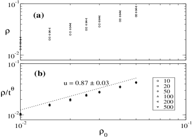
Figure 2: (a) Log-log plots of $\rho$ versus $\rho_{0}$ obtained for times $t=10,20,50,100,200$, and $500$ (from bottom to top). (b) Scaling plot of the curves shown in (a) using equation (11).

On the other hand, replacing $\frac{x_{0}}{z}=\frac{\theta+\delta}{u}$ in equation (8) one obtains

$$\rho(t,\rho_{0})=t^{-\delta}\Phi(\rho_{0}t^{\frac{\theta+\delta}{u}}).$$ (12)

The shape of the scaling function $\Phi$ is shown in figure 3 and the excellent data collapse obtained by plotting the data already shown in figure 1, strongly supports the formulated scaling hypothesis and the calculated exponents. In fact, the best fit of the data obtained, for $\rho_{0}\rightarrow 0$, gives $u=0.89(3)$ (see dotted line covering two decades in figure 3) that is in agreement with the preliminary estimation already performed with the data shown in figure 2 (covering less than one decade).

Also, the scaling of the initial density can also be obtained by replacing $b=\rho_{0}^{-1/x_{0}}$ in equation (1), giving

$$\rho(t,\rho_{0})=\rho_{0}^{\aleph/x_{0}}\Omega(t\rho_{0}^{z/x_{0}}),$$ (13)

where $\Omega$ is a scaling function that, for $t\rightarrow 0$ and $\rho_{0}\rightarrow 0$, can be approximated by $\Omega(x)\rightarrow x^{v}$ ($x\rightarrow 0$), where $v$ is an exponent. Thus one obtains

$$\rho(t,\rho_{0})=\rho_{0}^{\aleph/x_{0}+v\frac{z}{x_{0}}}t^{v}.$$ (14)

Now, by comparing equation (14) with equation (11) it follows that $v=\theta$ and $u=\frac{\aleph}{x_{0}}+v\frac{z}{x_{0}}$. Hence,

$$\frac{\aleph}{x_{0}}=\frac{\aleph/z}{x_{0}/z}=\frac{u\delta}{\delta+\theta}$$ (15)

Then, using $\frac{x_{0}}{z}=\frac{\theta+\delta}{u}$ and equation (15), one has that equation (13) can be written in terms of already measured exponents, so

$$\rho(t,\rho_{0})=\rho_{0}^{\frac{u\delta}{\delta+\theta}}\Omega(t\rho_{0}^{\frac{u}{\delta+\theta}}).$$ (16)

Figure 4 shows plots of the numerical data performed according to equation (16). The shape of the scaling function $\Omega$ can be observed and the collapse of the curves also supports the formulated scaling hypothesis.

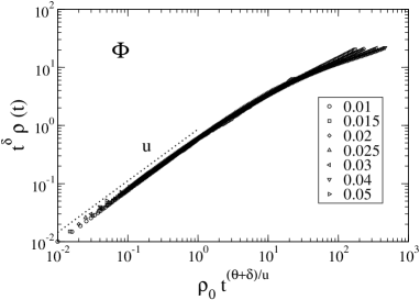
Figure 3: Scaling plot of the data shown in figure 1 obtained by using equation (12) for the time-scaling behavior. The dotted line -slightly shifted up for the sake of clarity- with slope $u=0.89$ corresponds to the best fit of the data obtained for the lowest density.

Figure 4: Scaling plot of the data shown in figure 1 obtained by using equation (16) for the scaling of the initial density.

Valuable information on the dynamic behavior of the system can also be obtained by measuring the temporal autocorrelation of the state of the site ($A(t,t_{0})$, averaged over all sites) that is expected to decay according to a power law Schmittman ; Huse , namely

$$A(t_{0},t)=\langle\sigma_{i}(t_{0})\sigma_{i}(t)\rangle-\langle\sigma_{i}(t_{0})\rangle\langle\sigma_{i}(t)\rangle\sim t^{-C_{a}}$$ (17)

where $\sigma_{i}(t)=1,0$ is the state of the site at time $t$. Also Huse

$$C_{a}=d/z-\theta.$$ (18)

Figure 5 shows log-log plots of the autocorrelation versus $t$ obtained using very low initial densities since equation (17) is expected to hold for $\rho_{0}\rightarrow 0$. From these plots one determines $C_{a}=0.35(2)$, and replacing this value in equation (18) the dynamic exponent $z=2.13(5)$ is obtained. Then by using equation (7) we obtain $D=2.42(5)$. These exponent values are in agreement with those already published in the literature that were obtained within the SOC regime paczuski , i.e., $z=2.1(5)$ and $D=2.43(1)$. Furthermore, equation (9) can be tested, yielding $D-1=1.42(5)$ (left-hand side) and $z/x_{0}=u/(\theta+\delta)=1.47(5)$ (right-hand side).

Now, we can discuss the relationship between short-time dynamic measurements and the behavior of relevant distributions characterizing return times of the activity to a given point in space. In fact, the distribution $P_{ALL}(0,t_{\parallel})$ is the probability for the activity at time $t_{\parallel}$ to revisit a site that was visited at time $0$ and is often referred to as the distribution of all return times paczuski . For $t_{\parallel}\gg 1$ such a distribution decays as a power law of the form $P_{ALL}(0,t_{\parallel})\propto t_{\parallel}^{-\tau_{ALL}}$, where $\tau_{ALL}$ is the ’lifetime’ exponent for all returns of the activity paczuski . Then, considering that $A(0,t)$ is the probability that a given site being occupied at $t=0$ returns to be occupied at time $t$, one has that $A(0,t)\propto P_{ALL}(0,t_{\parallel})$ since a site can change its state only when such a site, or any of its two neighbours, are visited by the activity. Then, by recalling that we are working in terms of the discrete sequential time $t$ such as $t_{\parallel}\propto t^{1-\theta}$ note1 , one has

$$A(t,0)\sim t^{-(1-\theta)\tau_{ALL}},\qquad\text{with}\qquad\tau_{ALL}\equiv\frac{C_{a}}{1-\theta}.$$ (19)

By means of short-time dynamic measurements we have obtained $\tau_{ALL}=0.39(4)$, in excellent agreement with the value calculated within the stationary state ($t>10^{6}$), given by $\tau_{ALL}=0.42(2)$ paczuski .

Summing up, the proposed dynamic scaling Ansatz for the approach to the stationary state generalizes the concepts previously developed to describe the critical dynamics of model A for systems exhibiting SOC. The dynamic scaling behavior was tested with the BS model showing that it holds for the density of sites with fitness below the critical one. Remarkably the exponents calculated by using the dynamic approach are in excellent agreement with those already measured within the stationary state. Using well established relationships between exponents and considering that only two of them are basic, the dynamic measurement allows the self-consistent evaluation of all exponents of the BS model. So, we have shown that the dynamic approach to the SOC regime is indeed critical and it is governed by the dynamic exponent $z$, standard exponents (i.e., those available from stationary determinations), and by the exponent $\theta$ that is introduced to describe the initial increase of the density. It is worth emphasizing that the criticality observed in the approach to the SOC state not only addresses new and challenging theoretical aspects of SOC behavior, but also is of great practical importance for the determination of relevant exponents.

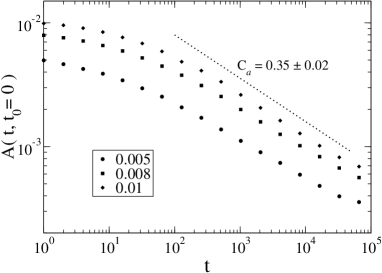
Figure 5: Log-log plots of the temporal autocorrelation versus $t$ obtained for different values of $\rho_{0}$. The dotted line with slope $C_{a}=0.35$ has been drawn for the sake of comparison.

References

- (1) P. Bak, C. Tang and K. Wiesenfeld, Phys. Rev. Lett. 59, 381 (1987), Phys. Rev. A. 38, 364 (1988).
- (2) P. Bak, How Nature Works. Copernicus. Springer-Verlag, New York. (1996).
- (3) H, J. Jensen. Self-Organized Criticality. Cambridge University Press. Cambridge. (1998).
- (4) H. K. Janssen, B. Schaub and B. Schmittmann, Z. Phys. B. 73, 539 (1989).
- (5) D. A. Huse, Phys. Rev. B. 40, 304 (1989), K. Humayun and A. J. Bray, J. Phys. A. (Math. and Gen.) 24, 1915 (1991), P. Grassberger, Physica A 214, 547 (1995) and L. Shulke and B. Zheng, Phys. Lett. A 204, 295 (1995). For reviews see B. Zheng, Int. J. of Mod. Phys. B. 12, 1419 (1998) and Physica A 283, 80 (2000).
- (6) P. Bak and K. Sneppen, Phys. Rev. Lett. 71, 4083 (1993).
- (7) H. Flyvbjerg, K. Sneppen and P. Bak, Phys. Rev. Lett. 71, 4087 (1993).
- (8) K. Sneppen, P. Bak, H. Flyvbjerg and M. H. Jensen, Proc. Natl. Acad. Sci. U.S.A., 92, 5209 (1995), P. Bak and M. Paczuski, ibid 92, 6689 (1995).
- (9) M. Paczuski, S. Maslov and P. Bak, Phys. Rev. E 53, 414 (1996).
- (10) Notice that in magnetic systems the time scale of the initial increase of the magnetization is set by , where is the initial magnetization Huse .
- (11) The relevant time scales involved are discussed in connection to equations (5) and (6).