Synchronization; coupled oscillators Time series analysis

Generalized synchronization onset

Abstract

The behavior of two unidirectionally coupled chaotic oscillators near the generalized synchronization onset has been considered. The character of the boundaries of the generalized synchronization regime has been explained by means of the modified system approach.

Chaotic synchronization is one of the fundamental nonlinear phenomena actively studied recently [1]. Several different types of chaotic synchronization of coupled oscillators, i.e. generalized synchronization (GS) [2], phase synchronization (PS) [1], lag synchronization (LS) [3], complete synchronization (CS) [4] and time scale synchronization (TSS) [5] are well known. There are also attempts to find unifying framework for chaotic synchronization of coupled dynamical systems [6, 7, 8, 9].

One of the interesting and intricate types of the synchronous behavior of unidirectionally coupled chaotic oscillators is the generalized synchronization. The presence of GS between the response $\mathbf{x}_{r}(t)$ and drive $\mathbf{x}_{d}(t)$ chaotic systems means that there is some functional relation ${\mathbf{x}_{r}(t)=\mathbf{F}[\mathbf{x}_{d}(t)]}$ between system states after the transient finished. This functional relation $\mathbf{F}[\cdot]$ may be smooth or fractal. According to the properties of this relation, GS may be divided into the strong synchronization and weak synchronization, respectively [10]. There are several methods to detect the presence of GS between chaotic oscillators, such as the auxiliary system approach [11] or the method of nearest neighbors [2, 12]. It is also possible to calculate the conditional Lyapunov exponents (CLEs) [13, 10] to detect GS. The regimes of LS and CS are also the particular cases of GS.

One of the interesting aspects of the generalized synchronization study is the analysis of the onset of this regime. In particular, the intermittent behavior is known to be revealed on the onset of GS [14, 15] as well as in case of the lag [3, 16, 17] or phase [18, 19, 20] synchronization.

At the same time, there are known examples of the unidirectionally coupled chaotic systems for which the location of the generalized synchronization onset on the “parameter mismatch — coupling strength” plane differs radically from the other synchronization types. Indeed, for two unidirectionally coupled Rössler oscillators with identical control parameters the value of the coupling strength corresponding to the onset of GS is twice as much as for the same oscillators with parameters detuned sufficiently [21]. For two unidirectionally coupled one–dimensional complex Ginzburg–Landau equations with sufficiently detuned control parameters the threshold of the GS regime onset does not depend on the value of the drive system parameter when the response system parameters are fixed [22]. Alternatively, for all other types of chaotic synchronization the dependence of the threshold of the synchronous regime arising on the value of the control parameter mismatch behaves in the different way, i.e. when the control parameter mismatch decreases the coupling parameter value corresponding to the onset of the synchronous regime also declines.

This letter aims to explain the mechanisms resulting in the generalized synchronization arising in the unidirectionally coupled chaotic oscillators and determining the location of the GS onset.

The causes of the generalized synchronization arising may be clarified by means of a modified system approach proposed in [23]. Let us consider the behavior of two unidirectionally coupled chaotic oscillators with slightly mismatched parameters

$$\begin{array}[]{l}\mathbf{\dot{x}}_{d}=\mathbf{H}(\mathbf{x}_{d},\mathbf{g}_{d})\\ \mathbf{\dot{x}}_{r}=\mathbf{H}(\mathbf{x}_{r},\mathbf{g}_{r})+\varepsilon\mathbf{A}(\mathbf{x}_{d}-\mathbf{x}_{r}),\end{array}$$ (1)

where $\mathbf{x}_{d,r}$ are the state vectors of the drive and response systems, respectively; $\mathbf{H}$ defines the vector field of the considered systems, $\mathbf{g}_{d}$ and $\mathbf{g}_{r}$ are parameters vectors, $\mathbf{A}={\{\delta_{ij}\}}$ is a coupling matrix ($\delta_{ii}=0$ or $1$, $\delta_{ij}=0$ ($i\neq j$)), $\varepsilon$ is a scale parameter characterizing the coupling strength.

In this case one can see that the response system $\mathbf{x}_{r}(t)$ may be considered as a modified system

$$\mathbf{\dot{x}}_{m}(t)=\mathbf{H}^{\prime}(\mathbf{x}_{m}(t),\varepsilon)$$ (2)

(where $\mathbf{H}^{\prime}(\mathbf{x}(t))=\mathbf{H}(\mathbf{x}(t))-\varepsilon\mathbf{A}\mathbf{x}(t)$) under the external force $\varepsilon\mathbf{A}\mathbf{x}_{d}(t)$:

$$\mathbf{\dot{u}}_{m}(t)=\mathbf{H}^{\prime}(\mathbf{u}_{m}(t),\varepsilon)+\varepsilon\mathbf{A}\mathbf{x}_{d}(t),$$ (3)

It is easy to see that the term $-\varepsilon\mathbf{A}\mathbf{x}(t)$ brings the additional dissipation into the system (2). Indeed, the phase flow contraction is characterized by means of the vector field divergence. Obviously, the vector field divergences of the modified and the response systems are related with each other as

$$\mathrm{div}\,\mathbf{H}^{\prime}=\mathrm{div}\,\mathbf{H}-\varepsilon\sum\limits_{i=1}^{N}\delta_{ii}$$ (4)

(where $N$ is the dimension of the modified system phase space), respectively. So, the dissipation in the modified system is greater than in the response one and it increases with the growth of the coupling strength $\varepsilon$.

The generalized synchronization regime arising in (1) may be considered as a result of two cooperative processes taking place simultaneously. The first of them is the growth of the dissipation in the system (2) and the second one is an increase of the amplitude of the external signal. Evidently, both processes are correlated with each other by means of parameter $\varepsilon$ and can not be realized in the coupled oscillator system (1) independently. Nevertheless, it is clear, that an increase of the dissipation in the modified system (2) results in the simplification of its behavior and the transition from the chaotic oscillations to the periodic ones. Moreover, if the additional dissipation is large enough the stationary fixed state may be realized in the modified system. On the contrary, the external chaotic force $\varepsilon\mathbf{A}\mathbf{x}(t)$ tends to complicate the behavior of the modified system and impose its own dynamics on it. Obviously, the generalized synchronization regime may not appear unless own chaotic dynamics of the modified system is suppressed.

Note also, that the onset of GS is determined by the stability of the periodic regimes of the modified system (2) which does not seem to depend on the mismatch of the control parameters $\mathbf{g}_{d,r}$ of the unidirectionally coupled oscillators. The stability of the periodical regimes is caused by the property of the modified system only. Therefore, the value of $\varepsilon_{GS}$ is not supposed to depend greatly on the parameter mistuning. Nevertheless, the sensitive dependence of the coupling strength value $\varepsilon_{GS}$ corresponding to the onset of GS on the control parameter mismatch may take place as it has been discussed above (see also [21]).

To explain the mechanisms causing such dependence of the coupling strength on the control parameter mismatch let us consider two unidirectionally coupled Rössler oscillators

$$\begin{array}[]{ll}\dot{x}_{d}=-\omega_{d}y_{d}-z_{d},&\dot{x}_{r}=-\omega_{r}y_{r}-z_{r}+\varepsilon(x_{d}-x_{r}),\\ \dot{y}_{d}=\omega_{d}x_{d}+ay_{d},&\dot{y}_{r}=\omega_{r}x_{r}+ay_{r},\\ \dot{z}_{d}=p+z_{d}(x_{d}-c),\mbox{\qquad\qquad\qquad}&\dot{z}_{r}=p+z_{r}(x_{r}-c),\\ \end{array}$$ (5)

where $\varepsilon$ is a coupling parameter. The control parameter values have been selected by analogy with [21] as $a=0.15$, $p=0.2$, $c=10.0$. The $\omega_{r}$–parameter determining the main frequency of the response system has been selected as $\omega_{r}=0.95$, and the analogous parameter $\omega_{d}$ of the drive system has been varied in the range from 0.8 to 1.1 providing the slight mismatch of the interacting oscillators.

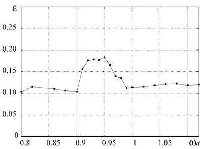
Figure 1: The boundary of the GS onset on the $(\omega_{d},\varepsilon)$ parameter plane for two unidirectionally coupled Rössler systems (5). The $\omega$–parameter of the response system has been fixed as $\omega_{r}=0.95$.

The boundary of the GS regime in system (5) on the $(\omega_{d},\varepsilon)$–plane is shown in Fig. 1. The GS onset has been detected by the conditional Lyapunov exponent computation [10] and verified by the auxiliary system method [11]. The threshold of the GS arising appears to be essentially higher for the small control parameter detuning of the considered systems rather than for the large ones. At the same time, if the parameter mismatch $(\omega_{d}-\omega_{r})$ is large enough, the coupling strength value $\varepsilon_{GS}$ corresponding to the GS regime onset is almost independent on the value $\omega_{d}$ of the drive system (see Fig. 1).

Such system behavior may be explained by means of the modified system method discussed in detail above. The response system (5) can be reduced to the modified system

$$\begin{array}[]{l}\dot{x}_{m}=-\omega_{r}y_{m}-z_{m}-\varepsilon^{*}x_{m},\\ \dot{y}_{m}=\omega_{r}x_{m}+ay_{m},\\ \dot{z}_{m}=p+z_{m}(x_{m}-c).\end{array}$$ (6)

To separate the discussed above different mechanisms resulting in the GS arising the $\varepsilon^{*}$ parameter has been used instead of $\varepsilon$.

In Fig 2 the bifurcation diagram for the modified system (6) is shown. It is clear that with the increase of the $\varepsilon^{*}$ parameter this system undergoes the transition from the chaotic to periodic oscillations through the inverse cascade of the period doubling. One can easily see, that starting from the value $\varepsilon^{*}_{p}\approx 0.06$ the periodic oscillations take place in the modified system (6). So, if the $\varepsilon^{*}$ parameter value is large enough the autonomous modified system displays the periodic oscillations.

To study the GS arising the non-autonomous dynamics of the modified system (6)

$$\begin{array}[]{l}\dot{x}_{m}=-\omega_{r}y_{m}-z_{m}-\varepsilon^{*}x_{m}+\varepsilon F(t),\\ \dot{y}_{m}=\omega_{r}x_{m}+ay_{m},\\ \dot{z}_{m}=p+z_{m}(x_{m}-c),\end{array}$$ (7)

should be considered, the time series $x_{d}(t)$ of the drive system being used as the external force $F(t)$.

For the control parameters pointed above the Fourier spectrum of the drive system (5) is characterized by the single well–defined frequency component $f_{m}$. When varying the $\omega_{d}$-parameter the main frequency $f_{m}$ also changes. Therefore, the behavior of the modified system (7) under the external harmonic signal $F(t)=A\cos(2\pi f_{m}t)$ may be considered as the first approximation of the dynamics of two unidirectionally coupled chaotic oscillators (5). The amplitude $A$ of the external harmonic signal $F(t)$ should correspond to the drive Rössler system behavior.

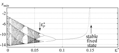
Figure 2: The bifurcation diagram of the modified Rössler system (6) versus the parameter $\varepsilon^{*}$. The value of the parameter $\varepsilon^{*}$ when the modified system starts demonstrating the periodic dynamics is shown by an arrow.

Obviously, when the main frequency of the response system and the frequency $f_{m}$ of the external signal are close enough with each other the frequency entrainment may take place resulting in the synchronization. In this case the behavior of the modified system (and the response one, respectively) may be different qualitatively inside the synchronization tongue and outside it. The location of the boundaries of the GS regime (see Fig. 1) confirms this assumption. When the parameter mismatch of the considered response and drive oscillators is large enough (the main frequencies are not entrained and the system (7) is outside of the synchronization tongue) the GS regime onset is observed practically for the same value of the coupling strength $\varepsilon$ independently of the $\omega_{d}$ parameter value. In this case the threshold of the GS regime arising is defined mainly by the properties of the modified system (7). Obviously, the features of the GS onset location for the small mistuning of the control parameters may be defined by the system dynamics inside the synchronization tongue.

Let us consider the behavior of the non-autonomous modified system (7) under the external harmonic signal in detail. The value of the $\varepsilon^{*}$ parameter has been fixed as $\varepsilon^{*}=0.11$ that corresponds approximately to the threshold of the GS arising when the control parameters of the coupled Rössler oscillators are detuned sufficiently. The amplitude of the external harmonic signal has been used in the form $A=\varepsilon B$, the value of $B$ parameter has been selected as $B\approx 0.105$ for the levels of the energy of the harmonic signal $F(t)=A\cos(2\pi f_{m}t)$ and the main spectral component of the Fourier spectrum of the drive system $\mathbf{x}_{d}(t)$ to be equal. In this case the $\varepsilon$ parameter determines the intensity of the external influence on the modified system and may be considered as a quantity corresponding to the coupling strength of the coupled oscillators (5). Such normalization allows us to mark the synchronization region of the non-autonomous modified system on the $(\omega_{d},\varepsilon)$ directly.

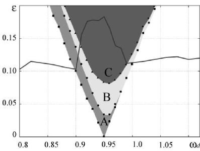
Figure 3: The synchronization tongue of the non-autonomous modified system under the external harmonic signal on the $(\omega_{d},\varepsilon)$ plane. The area of the period–2 regime (marked by the letter “B”) as well as the region of the chaotic oscillations (marked by “C”) inside the synchronization tongue are shown by the different colors. The boundary of the GS onset (compare with Fig. 1) has also been shown.

The synchronization tongue of the non-autonomous modified system (7) on the $(\omega_{d};\varepsilon)$ plane is shown in Fig. 3. The region A presents the set of the parameter values corresponding to the periodic oscillation regime with the frequency $f_{m}$ of the external harmonic signal. With the increase of the $\varepsilon$ parameter value inside this region the system undergoes the transition to chaotic behavior through the cascade of the period doubling. The region C corresponds to the chaotic oscillations, while the area B presents the parameter values of the period doubling cascade. The boundary of the GS regime is also shown in Fig. 3 for the cause of the dependence of the GS arising threshold $\varepsilon_{GS}$ on the control parameter mismatch to be explained clearly. One can see easily, that the behavior of the response system differs essentially inside and outside the synchronization tongue of the modified system.

Let us consider briefly the cause of such location of the GS onset. The external signal (chaotic time series of the drive Rössler system or the simulating harmonic signal) excites the proper chaotic dynamics of the modified system. Therefore, for the considered coupled Rössler systems the GS regime starts being destroyed with the growth (inside the synchronization tongue) of the $\varepsilon$ parameter. To suppress the chaotic oscillations in the modified system the value of the dissipation $\varepsilon^{*}$ should be increased. As in the coupled systems (5) the coupling strength $\varepsilon$ plays simultaneously the role both of the dissipation and of the intensity of the drive system signal, the suppression of the proper chaotic dynamics of the response system takes place for the more larger values of the parameter $\varepsilon$. Therefore, the threshold of the GS regime arising is shifted towards the large values of the coupling strength $\varepsilon$.

Comparing the boundary of the GS regime in the coupled Rössler systems (5) with the location of the synchronization tongue of the non-autonomous modified system (7) under the external harmonic signal on the $(\omega_{d},\varepsilon)$ plane it is necessary to take into account that the synchronization area has been obtained for the fixed value of the parameter $\varepsilon^{*}$. Moreover, the chaotic dynamics of the drive system influencing on the location of the GS onset has also been eliminated from the consideration. Therefore, this synchronization tongue on the $(\omega_{d},\varepsilon)$ plane has only the qualitative character allowing to explain the mechanisms resulting in the GS onset features.

In conclusion, we have explained the peculiarity of the GS onset in the unidirectionally coupled Rössler oscillators by means of the modified system dynamics consideration. The character of the GS onset location is determined by the entrainment (or, on the contrary, by the absence of it) of the main frequencies of the Fourier spectra of the interacting systems. Inside the synchronization tongue the GS onset may be shifted towards the large values of the coupling strength if the external influence excites the proper chaotic dynamics inside the area of the main frequencies entrainment. It is important to note that this conclusion has been made for the chaotic systems with a distinct main frequency in the power spectrum, so, the discussed phenomena and the presented arguments are specific to such systems. Indeed, the mechanism discussed above is determined by the interaction of the main spectral components of coupled chaotic oscillators. Probably, one can expect that the phenomenon of the increase of the coupling strength $\varepsilon_{GS}$ corresponding to the onset of the generalized synchronization regime for the identical parameter values in comparison with the detuned ones may not be observed for the system with broad power spectra without distinct main frequency.

- [1] \NamePikovsky A., Rosenblum M. Kurths J. \BookSynchronization: a universal concept in nonlinear sciences \PublCambridge University Press \Year2001.
- [2] \NameRulkov N.F., Sushchik M.M., Tsimring L.S. Abarbanel H.D.I. \REVIEWPhys. Rev. E511995980.
- [3] \NameRosenblum M.G., Pikovsky A.S. Kurths J. \REVIEWPhys. Rev. Lett.7819974193.
- [4] \NamePecora L.M. Carroll T.L. \REVIEWPhys. Rev. Lett.641990821.
- [5] \NameHramov A.E. Koronovskii A.A. \REVIEWPhysica D2062005252.
- [6] \NameBrown R. Kocarev L. \REVIEWChaos102000344.
- [7] \NameBoccaletti S., Kurths J., Osipov G., Valladares D.L. Zhou C.S. \REVIEWPhysics Reports36620021.
- [8] \NameBoccaletti S., Pecora L.M. Pelaez A. \REVIEWPhys. Rev. E632001066219.
- [9] \NameHramov A.E. Koronovskii A.A. \REVIEWChaos142004603.
- [10] \NamePyragas K. \REVIEWPhys. Rev. E541996R4508.
- [11] \NameAbarbanel H.D.I., Rulkov N.F. Sushchik M.M. \REVIEWPhys. Rev. E5319964528.
- [12] \NamePecora L.M., Carroll T.L. Heagy J.F. \REVIEWPhys. Rev. E5219953420.
- [13] \NamePecora L.M. Carroll T.L. \REVIEWPhys. Rev. A4419912374.
- [14] \NameHramov A.E. Koronovskii A.A. \REVIEWEurophysics Letters442005169.
- [15] \NameZhan M., Wang X., Gong X., Wei G.W. Lai C.-H. \REVIEWPhys. Rev. E682003036208.
- [16] \NameBoccaletti S. Valladares D.L. \REVIEWPhys. Rev. E6220007497.
- [17] \NameZhan M., Wei G.W. Lai C.H. \REVIEWPhys. Rev. E652002036202.
- [18] \NamePikovsky A., Osipov G., Rosenblum M., Zaks M. Kurths J. \REVIEWPhys. Rev. Lett.79199747.
- [19] \NamePikovsky A., Zaks M., Rosenblum M., Osipov G. Kurths J. \REVIEWChaos71997680.
- [20] \NameLee K.J., Kwak Y. Lim T.K. \REVIEWPhys. Rev. Lett.811998321.
- [21] \NameZheng Z. Hu G. \REVIEWPhys. Rev. E6220007882.
- [22] \NameHramov A.E., Koronovskii A.A. Popov P.V. \REVIEWPhys. Rev. E722005037201.
- [23] \NameHramov A.E., Koronovskii A.A. \REVIEWPhys. Rev. E712005067201.