The Domain Chaos Puzzle and the Calculation of the Structure Factor and Its Half-Width

Abstract

The disagreement of the scaling of the correlation length $\xi$ between experiment and the Ginzburg-Landau (GL) model for domain chaos was resolved. The Swift-Hohenberg (SH) domain-chaos model was integrated numerically to acquire test images to study the effect of a finite image-size on the extraction of $\xi$ from the structure factor (SF). The finite image size had a significant effect on the SF determined with the Fourier-transform (FT) method. The maximum entropy method (MEM) was able to overcome this finite image-size problem and produced fairly accurate SFs for the relatively small image sizes provided by experiments.

Correlation lengths often have been determined from the second moment of the SF of chaotic patterns because the functional form of the SF is not known. Integration of several test functions provided analytic results indicating that this may not be a reliable method of extracting $\xi$. For both a Gaussian and a squared SH form, the correlation length $\overline{\xi}\equiv 1/\sigma$, determined from the variance $\sigma^{2}$ of the SF, has the same dependence on the control parameter $\varepsilon$ as the length $\xi$ contained explicitly in the functional forms. However, for the SH and the Lorentzian forms we find $\overline{\xi}\sim\xi^{1/2}$.

Results for $\xi$ determined from new experimental data by fitting the functional forms directly to the experimental SF yielded $\xi\sim\varepsilon^{-\nu}$ with $\nu\simeq 1/4$ for all four functions in the case of the FT method, but $\nu\simeq 1/2$, in agreement with the GL prediction, in the the case of the MEM. Over a wide range of $\varepsilon$ and wave number $k$, the experimental SFs collapsed onto a unique curve when appropriately scaled by $\xi$.

I Introduction

Spatially extended nonlinear non-equilibrium systems continue to be of great interest because they yield qualitatively different phenomena that do not occur in linear systems CH93 . One of these phenomena is spatio-temporal chaos. The examples of spatio-temporal chaos found in Rayleigh-Bénard convection (RBC) lend themselves to particularly detailed experimental study under exceptionally well controlled external conditions BPA00 . RBC occurs in a thin horizontal layer of fluid with thickness $d$ heated from below when the temperature difference $\Delta T$ exceeds a critical value $\Delta T_{c}$ SC .

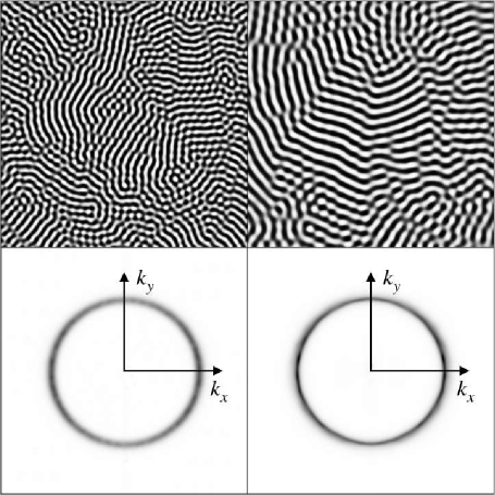
Figure 1: All images are for $\Omega=17.7$ and $\varepsilon=0.05$. Upper left: shadowgraph image of size $60d\times 60d$ from $\Gamma=61.5$. A movie is available MOV1 . Upper right: shadowgraph image of size $44d\times 44d$ from $\Gamma=36$. Lower left: the average SF $S\left(k_{x},k_{y}\right)$ computed using the FT method and a Kaiser-Bessel window with $\alpha=2.5$ and averaged over 4096 images like the one in the upper left. Lower right: the average SF from same data as shown in lower left, except $S\left(k_{x},k_{y}\right)$ was computed with the MEM.

Particularly noteworthy is the state that occurs in RBC when the fluid layer of density $\rho$ and shear viscosity $\eta$ is rotated about a vertical axis with angular frequency $\omega$. When the dimensionless frequency $\Omega\equiv\omega d^{2}\rho/\eta$ exceeds a critical value, then the pattern immediately above onset consists of disordered domains of convection rolls known as domain chaos. This is illustrated in Fig. 1a and 1b. Within each domain the roll orientation is more or less uniform; but different domains have different orientations KL1 ; KL2 ; CB1 ; HB ; BH ; HEA1 ; HEA2 ; HPAE98 . The domains are unstable and undergo a persistent but irregular dynamics. In this case, the time-averaged mean-square velocities and temperature deviations from the conduction state grow continuously from zero as $\Delta T_{c}$ is exceeded, i.e. the bifurcation is supercritical.

Chaos immediately above a supercritical bifurcation offers a unique opportunity for theoretical study because weakly-nonlinear theories are expected to be applicable. These theories, in the form of Ginzburg-Landau (GL) or Swift-Hohenberg (SH) equations, by virtue of their general structure and from their numerical solutions, predict that the inverse half-width at half-height $\xi$ of the structure factor (SF, the power spectrum of the pattern) should vary as $\varepsilon^{-\nu}$ with $\nu=1/2$ as $\varepsilon\equiv\Delta T/\Delta T_{c}-1$ vanishes Friedrich ; Fantz ; Neufeld ; Cross ; CMT ; PPS97 ; PPS972 , and that it is the only length scale in the problem. Thus it was particularly disappointing that measurements for domain chaos disagreed with this expectation HEA1 . Determinations of a correlation length $\bar{\xi}$ based on the variance of the SF found $\bar{\xi}\propto\varepsilon^{-\nu_{eff}}$ with $\nu_{eff}\simeq 1/4$ rather than 1/2.

Several possible explanations of the apparent disagreement with theory were explored by various authors. Hu et al. proposed that defects and fronts injected by the side wall into the bulk may play an important role HPAE98 . Laveder et al. demonstrated that additive white noise intended to mimic the effect of wall defects decreases $\nu$ to the value of $\nu_{eff}$ measured experimentally provided that the noise level is sufficiently large LPPS99 . Recent unpublished experiments in our group using a sample with a radially ramped spacing BMCA99 ; BMOA05 render the side-wall-injected defect idea an unlikely explanation. On the basis of numerical simulation using a SH equation Cross et al. proposed that the finite size of the experimental convection sample decreases the effective value of $\nu$ CLM01 .

Experimental determinations of a characteristic length scale $\overline{\xi}$ usually are based on numerical estimates of the variance $\sigma^{2}$ of the SF, with $\overline{\xi}=1/\sigma$ HEA1 ; MBCA93 . This is so because the precise analytic form of $S(k)$ is not known in the nonlinear regime above onset. In Sect. II we examine the relationship between $\overline{\xi}$ and the length $\xi$ that appears explicitly in various functional forms that might be used as approximations to the SF. We find that $\overline{\xi}\sim\xi^{1/2}$ when $\xi$ is the length appearing in the SF of the linear GL or SH equation. Thus, in those cases $\overline{\xi}$ does not have the same $\varepsilon$-dependence as $\xi$. However, we find that $\overline{\xi}\sim\xi$ for the square of the linear SH SF and for a Gaussian form for the SF. The results suggest that the success of the moment method of data analysis depends upon the rate at which the SF decreases at large $k$.

In Sect. III we discuss two methods of determining the SF from patterns. The standard method, using the Fourier power spectrum, is sensitive to the limited size of the experimental images FNsize . To overcome this limitation we also employed the maximum entropy method (MEM), which is discussed in detail in that section. The benefits of the MEM are exhibited through analysis of images from a SH simulation detailed in Sect. IV. We find that the MEM is quite powerful in its ability to overcome the finite image-size problem.

In Sect. V we present new experimental results for patterns in the domain-chaos state. We compare results from the Fourier analysis to the results from the MEM. We determined $\xi$ by fitting several possible functional forms for the SF to the data and found that the results for $\xi$ are not very sensitive to the form of the fitting function. In the case of the Fourier analysis, the fits did not change the result HEA1 $\nu\simeq 1/4$ that had been found before by the moment method. The reason why the moment method also gave this result can be found in the behavior of $S(k)$ at large $k$, where $S(k)$ drops off fast enough for $\overline{\xi}$ to be essentially proportional to $\xi$. In the case of the MEM, we found that $\nu\simeq 1/2$ as expected. This indicates that the findings from Fourier analysis are dominated by the finite image-size effect.

We also examined the maximum height $B$ of the SF and found $B\sim\varepsilon^{\beta}$ with $\beta\simeq 3/4$ in the case of Fourier analysis. The two results $\nu\simeq 1/4$ and $\beta\simeq 3/4$ conspire to retain the expected dependence of the total power on $\varepsilon^{\nu+\beta}$ with $\nu+\beta=1$ even though both $\nu$ and $\beta$ do not have the expected value 1/2. Once again, we find that the MEM overcomes the finite data length yielding $\beta\simeq 1/2$. We also find that the result for $\nu$ and $\beta$ are not strongly dependent on $\Omega$ for either the Fourier analysis or the MEM. Thus we conclude that, in light of careful analysis using the MEM, the experimental domain-chaos state does possess a length scale in agreement with the prediction from the GL model.

Finally, in Sect. VI, we examine the extent to which the SF can be represented by a unique scaling function over a range of $\varepsilon$ and $k$. We obtain excellent collapse of the data, both in the case of Fourier analysis and the MEM, when the results for $\xi$ obtained from a fit to the SF at each $\varepsilon$ are used to scale the SF.

II Moments of Analytic Functions

In order to better understand the consequences of using numerical moments to compute the correlation length, we derived analytic expressions for the zeroth, first, and second moments of several proposed forms of the SF. This yielded results for the correlation length $\overline{\xi}$ based on moments that could be compared with the correlation length $\xi$ that occurs directly in the functional form chosen for the SF. We found that the $\overline{\xi}\sim\xi^{m}$ where $m$ depended on the particular form of the structure factor. This suggests that using moments to measure the correlation length does not necessarily yield $\overline{\xi}$ with the $\varepsilon$ dependence implied by the GL model.

We investigated four particular forms of the SF. The exact form for domain chaos is not known. For our purposes one useful form is the SF of the linear SH equation

$$S\left(k\right)=\frac{4k_{0}^{2}B}{\xi^{2}\left(k^{2}-k_{0}^{2}\right)^{2}+4k_{0}^{2}}\textrm{.}$$ (1)

It is an excellent approximation to the SF of the linearized full equations of motion (the Boussinesq equations) in the presence of additive noise for RBC below onset OS02 . Another useful form is the squared SH SF

$$S\left(k\right)=\left[\frac{4k_{0}^{2}\sqrt{B}}{\xi_{s}^{2}\left(k^{2}-k_{0}^{2}\right)^{2}+4k_{0}^{2}}\right]^{2}$$ (2)

used by some authors for fits to numerical results in order to estimate a half width at half height $\delta k$ of the distribution sqSH ; sqSH2 . In the limit of large $\xi$, the correlation length $\xi$ in Eq. 1 approaches $1/\delta k$, but $\xi_{s}$ in Eq. 2 approaches $\sqrt{\sqrt{2}-1}/\delta k$ for large $\xi_{s}$. When we directly compare $\xi$ and $\xi_{s}$, as in Fig. 16 below, we divide $\xi_{s}$ by $\sqrt{\sqrt{2}-1}$ so that it approaches $1/\delta k$.

We also considered a Gaussian form

$$S\left(k\right)=B\exp\left[-\left(\ln 2\right)\left(k-k_{0}\right)^{2}\xi^{2}\right]$$ (3)

and a Lorentzian form

$$S\left(k\right)=\frac{B}{\xi^{2}\left(k-k_{0}\right)^{2}+1}\textrm{.}$$ (4)

The latter is the SF of the one-dimensional linearized GL equation. The correlation length $\xi$ of both the Gaussian and the Lorentzian is exactly equal to $1/\delta k$ regardless of the size of $\xi$. For all four of these functions we note that the position of the peak of $S\left(k\right)$ is at $k_{0}$ and $S\left(k_{0}\right)=B$.

The total power is $P=2\pi\int_{0}^{\infty}S\left(k\right)kdk$. In the case of the SH form,

$$P=\frac{2\pi k_{0}B}{\xi}\left[\frac{\pi}{2}-\tan^{-1}\left(-\frac{\xi k_{0}}{2}\right)\right]$$ (5)

which reduces to

$$P=\frac{2\pi^{2}k_{0}B}{\xi}\left[1-\frac{2}{\pi\xi k_{0}}+\mathcal{{O}}\left(\frac{1}{\xi^{3}}\right)\right]$$ (6)

in the limit of large $\xi$. In the case of the squared SH form,

$$P=2\pi k_{0}^{2}B\left\{\frac{1}{4+\xi_{s}^{2}k_{0}^{2}}+\frac{1}{2\xi_{s}k_{0}}\left[\frac{\pi}{2}-\tan^{-1}\left(-\frac{\xi_{s}k_{0}}{2}\right)\right]\right\}$$ (7)

which reduces to

$$P=\frac{\pi^{2}k_{0}B}{\xi_{s}}\left[1+\mathcal{{O}}\left(\frac{1}{\xi_{s}^{3}}\right)\right]$$ (8)

in the limit of large $\xi_{s}$.

The first moment is $\overline{k}=(2\pi/P)\int_{0}^{\infty}S\left(k\right)k^{2}dk$.

In the case of the SH form

$$\overline{k}=k_{0}\frac{\frac{2}{\xi k_{0}}\sin\left[\frac{1}{2}\tan^{-1}\left(\frac{2}{\xi k_{0}}\right)\right]+\cos\left[\frac{1}{2}\tan^{-1}\left(\frac{2}{\xi k_{0}}\right)\right]}{\left(1+\frac{4}{\xi^{2}k_{0}^{2}}\right)^{1/4}\left[\frac{1}{2}-\frac{1}{\pi}\tan^{-1}\left(-\frac{\xi k_{0}}{2}\right)\right]}$$ (9)

which reduces to

$$\overline{k}=k_{0}\left[1+\frac{2}{\pi\xi k_{0}}+\mathcal{{O}}\left(\frac{1}{\xi^{2}}\right)\right]$$ (10)

in the limit of large $\xi$.

In the case of the squared SH form

$$\overline{k}=k_{0}\frac{\pi\sin\left[\frac{1}{2}\tan^{-1}\left(\frac{2}{\xi_{s}k_{0}}\right)\right]+\pi\xi_{s}k_{0}\cos\left[\frac{1}{2}\tan^{-1}\left(\frac{2}{\xi_{s}k_{0}}\right)\right]}{2\xi_{s}^{2}k_{0}^{2}\left(1+\frac{4}{\xi_{s}^{2}k_{0}^{2}}\right)^{1/4}\left(\frac{1}{4+\xi_{s}^{2}k_{0}^{2}}+\frac{1}{2\xi_{s}k_{0}}\left[\frac{\pi}{2}-\tan^{-1}\left(-\frac{\xi_{s}k_{0}}{2}\right)\right]\right)}$$ (11)

which reduces to

$$\overline{k}=k_{0}\left[1-\frac{1}{2\xi_{s}^{2}k_{0}^{2}}+\mathcal{{O}}\left(\frac{1}{\xi_{s}^{3}}\right)\right]$$ (12)

in the limit of large $\xi_{s}$.

The second moment does not converge for the SH form but it does for the squared SH form. In the case of squared SH, $\sigma^{2}\equiv\overline{k^{2}}-\overline{k}^{2}$, where

$$\overline{k^{2}}=k_{0}^{2}\frac{\frac{1}{\xi_{s}^{2}k_{0}^{2}}+\frac{1}{2\xi_{s}k_{0}}\left[\frac{\pi}{2}-\tan^{-1}\left(-\frac{\xi_{s}k_{0}}{2}\right)\right]}{\frac{1}{4+\xi_{s}^{2}k_{0}^{2}}+\frac{1}{2\xi_{s}k_{0}}\left[\frac{\pi}{2}-\tan^{-1}\left(-\frac{\xi_{s}k_{0}}{2}\right)\right]}$$ (13)

and Eq. 11 gives $\overline{k}^{2}$. For large $\xi_{s}$,

$$\sigma^{2}=\frac{1}{\xi_{s}^{2}}\left[1-\frac{8}{3\pi\xi_{s}k_{0}}+\mathcal{{O}}\left(\frac{1}{\xi_{s}^{2}}\right)\right]$$ (14)

so that $\overline{\xi}_{s}\sim\xi_{s}$.

In order to compute a similar expression for the SH form, we introduced a cutoff $k_{C}$ so that the second moment remained finite. In that case $\sigma^{2}=2\pi P^{-1}\int_{0}^{k_{C}}S\left(k\right)k^{3}dk-\overline{k}^{2}$ so that

$$\sigma^{2}=\frac{k_{0}^{2}\left\{\tan^{-1}\left(\frac{\xi}{2k_{0}}\left[k_{C}^{2}-k_{0}^{2}\right]\right)+\tan^{-1}\left(\frac{\xi k_{0}}{2}\right)\right\}+\frac{k_{0}}{\xi}\ln\left(\frac{4k_{0}^{2}+\xi^{2}\left[k_{C}^{2}-k_{0}^{2}\right]^{2}}{4k_{0}^{2}+\xi^{2}k_{0}^{4}}\right)}{\tan^{-1}\left(\frac{\xi k_{C}^{2}}{2k_{0}}-\frac{\xi k_{0}}{2}\right)-\tan^{-1}\left(-\frac{\xi k_{0}}{2}\right)}-\overline{k}^{2}$$ (15)

and in the limit of large $\xi$

$$\sigma^{2}\simeq\frac{1}{\xi}\left[\frac{k_{0}}{\pi}\ln\left(\frac{\left[k_{C}^{2}-k_{0}^{2}\right]^{2}}{k_{0}^{4}}\right)-\frac{4k_{0}}{\pi}\right]+\mathcal{{O}}\left(\frac{1}{\xi^{2}}\right)\textrm{.}$$ (16)

Equation 16 indicates that in the case of the SH form $\bar{\xi}\sim\sqrt{\xi}$ regardless of the cutoff $k_{C}$. Although we do not present the details here, we also found that $\overline{\xi}\sim\sqrt{\xi}$ for the Lorentzian form but $\overline{\xi}\sim\xi$ for the Gaussian form.

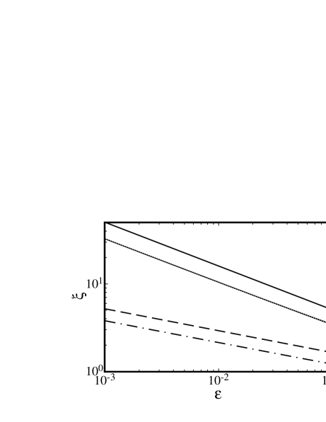
Figure 2: $\overline{\xi}$ computed from integration of the SH SF and the squared SH SF. The analytic results were evaluated with $\xi=1.6\varepsilon^{-1/2}$, $k=\pi$, and $k_{C}=14$. Solid line: $\xi=1.6\varepsilon^{-1/2}$ (chosen to match the solid line in Fig. 16). Dashed line: $\overline{\xi}$ from SH computed with Eq. 15 using $k_{C}=14$ and computing $\overline{k}$ numerically so that the integration is done only over the range $0<k<14$ for consistency. Dashed-dotted line: Approximate $\overline{\xi}$ from SH computed with Eq. 16. Dotted line: $\overline{\xi}_{s}$ computed from Eq. 11 and Eq. 13. Thin solid line that passes almost directly through dotted line: Approximate $\overline{\xi}_{s}$ from squared SH computed from Eq. 14.

Figure 2 compares these results for $\overline{\xi}$ computed by numerically integrating the SH SF and the squared SH SF. The lowest order expansion for the squared SH SF in Eq. 14 is an excellent approximation to the exact result as it lands almost directly on top of it. However, although the exponent is $-1/2$, it does give a $\overline{\xi}_{s}$ that is smaller than the input $\xi$ (shown as the solid line in Fig. 2) because of the extra constant $\sqrt{\sqrt{2}-1}$ discussed earlier. The approximate result for the SH SF (from Eq. 16) is not very close to the exact result (from Eq. 15) because the exact result for $\overline{k}$ (Eq. 9) was used to compute Eq. 16 while the dashed curve shown in Fig. 2 was computed with a finite cutoff for $\overline{k}$ to match the cutoff used in the integral for $\overline{k^{2}}$ for the sake of consistency. Nevertheless, the approximate result is parallel to the exact result with cutoff indicating that regardless of these details, the exponent from integrating the SH SF is $-1/4$.

According to the GL model, at small $\varepsilon$ one expects $\xi\sim\varepsilon^{-\nu}$ with $\nu=1/2$ Cross ; CMT . One also expects the total power to vanish at onset in proportion to $\varepsilon$. Thus, if Eq. 1 or Eq. 2 gives the shape of $S\left(k\right)$ correctly, then according to Eq. 6 or Eq. 8, $P\sim\varepsilon^{\nu+\beta}$with $\nu+\beta=1$ and $B\sim\varepsilon^{\beta}$ with $\beta=1/2$.

III Estimation of $S\left(k\right)$ from pattern images

We found that the accuracy of $S\left(k\right)$, estimated from the Fourier power spectrum, suffered greatly due to the finite size of the images of patterns that are available from experiment. In applying the Fourier-transform (FT) method to compute $S\left(k\right)$ from experimental data, we divided the images by a reference image taken below onset, applied a Kaiser-Bessel window KK66 to the divided images, and computed the magnitude squared of the FT. The azimuthal average of the squared magnitude of the FT yielded the SF $S\left(k\right)$.

We experimented with three windowing functions: a square window, a Welch window, and a Kaiser-Bessel window KK66

$$w_{KB}\left(t\right)=\left\{\begin{array}[]{cc}\textrm{I}_{0}\left(\pi\alpha\sqrt{1-\left[t/\tau\right]^{2}}\right)/\textrm{I}_{0}\left(\pi\alpha\right)&\left|t\right|<\tau\\ 0&\left|t\right|>\tau\ .\end{array}\right.$$ (17)

In Eq. 17 $t$ is the distance along one of the axes from the center, $\tau$ is the half-width of the image, and $\textrm{I}_{0}$ is the modified Bessel function of the first kind and order zero. The parameter $\alpha$ controls the rate at which the window drops off as the edge of the image is approached. Since the data was two dimensional, the window was the product of a one-dimensional window function in each direction. Since the windowing function attenuates the signal around the edges of the image, it reduces the total power. To compensate for this we divided $S\left(k\right)$ by a constant so that the total power in the final SF agreed with the total power of the raw image.

The specific windowing function did not greatly affect the result for $\xi$. We ultimately settled on using a Kaiser-Bessel window with $\alpha=2.5$ for the results given in this paper. Our major results, namely the exponents $\nu$ and $\beta$ and the scaling collapse of the SF, were independent of the windowing function.

We used a fast Fourier-transform (FFT) algorithm FFTW capable of transforming images of arbitrary size to compute the SF so that no interpolation or zero padding was required to re-size the image to an integer power of two. We found that interpolation distorts the large-$k$ behavior of the SF because it smooths out random noise that is present in the original signal. The use of zero padding circumvents the smoothing of the noise and thus avoids this distortion at large $k$, but instead inserts ringing at small $k$. Due to the easy availability of FFT algorithms that can work on any size image and the speed of modern computers, there is no reason to sacrifice the behavior of the SF at either large or small $k$. A minor tradeoff is that previous work utilized an aspect-ratio correction to the image that removed a slight anisotropy in the frame grabber Hu . Because this correction requires interpolation of the raw image we avoided using it. We expected only a very slight error by doing so because the raw images are nearly square. However, in the $\Gamma=36$ sample there was a radial distortion, due to optical aberration, that was strong enough to warrant its removal in order to avoid a systematic error in the length scale. We did not investigate the large $k$ behavior in that sample, so we expect no significant problem from the distortion correction.

Even after dividing the experimental images by an optical background, the resulting SF still contained the non-deterministic part of the background spectrum present in the images taken below onset. Since fluctuations WAC95 ; OA03 are too feeble to be detected for the parameters of the present experiment, we attributed this background signal primarily to electronic noise and subtracted a background, determined below onset, from the SF above onset. As a result, for the case of experimental data, the analysis that follows is applied to the background subtracted SF $\delta S\left(k\right)\equiv S\left(k\right)-S_{b}\left(k\right)$ where $S_{b}\left(k\right)$ is the SF averaged over many images below the onset. We also applied the FT to simulations of the SH domain-chaos model. In that case there was no need to divide by a reference image or to subtract electronic noise, so we used $S\left(k\right)$ computed directly from the simulation images.

We attempted to overcome the finite image-size problem of the FT method by using the maximum entropy method (MEM) to estimate $S\left(k\right)$. Although this method is commonly used for 1D data NR , computing the spectrum of 2D data with this technique is still somewhat of an open problem MEM3 . We implemented the algorithm detailed in Ref. MEM1 which uses an iterative method to arrive at the power-spectrum estimate. Figure 4 in Ref. MEM1 provides a detailed flowchart of the MEM algorithm, which we followed precisely. The MEM provides the power spectrum as an expansion of the form

$$S\left(k_{x},k_{y}\right)=\frac{1}{F\left[\lambda\left(n_{1},n_{2}\right)\right]},$$ (18)

where $\lambda\left(n_{1},n_{2}\right)$ are the coefficients of the expansion and $F\left[\cdots\right]$ is the discrete Fourier transform. Because the MEM provides an expansion containing sines and cosines in the denominator, in contrast with the FT where sines and cosines are in the numerator, the resulting power spectrum may more accurately represent sharp peaks because it may contain poles NR . It was also shown previously MEM2 that the MEM is much less sensitive to short data lengths than standard Fourier analysis.

The algorithm in Ref. MEM1 depends on an accurate estimate of the auto-correlation of the data. A central section is cut from the auto-correlation data and used in the iterative process. For all the analysis in the present work we used a region size of $45\times 45$ data points, which corresponded to about $12d\times 12d$ for the $\Gamma=61.5$ sample and also for the SH simulation. The iterative process produces auto-correlation data that is continued beyond this region according to the spectral-entropy maximization-criteria that defines the MEM. The number of coefficients $\lambda\left(n_{1},n_{2}\right)$ determines the size of the continued region. In principle it is possible to use a relatively small continued-region size, in order to reduce the required amount of computation, and then embed the resulting $\lambda\left(n_{1},n_{2}\right)$ into a larger region, setting higher order coefficients to zero in order to produce a finely meshed power spectrum. In practice we found that this approach, while advocated in Ref. MEM1 , did not always produce positive-definite power spectra and thus was not stable for our purposes. Instead we ran the entire algorithm on a large $720\times 720$ mesh for $\lambda\left(n_{1},n_{2}\right)$. Although this was heavily computation intensive, it did provide a reliable power spectrum estimate after a sufficient number of iterations. On our modest fleet of 2 GHz PowerMac G5s, we could run roughly 200 iterations per minute per CPU. Typically we needed 50,000 to 1 million iterations for convergence, depending on the $\varepsilon$ step, making the processing of all the data in the present work a fairly massive undertaking.

The number of iterations depended on the auto-correlation error $\epsilon_{0}$, as defined by Eq. 25 in Ref. MEM1 , which was reduced to a specified level. In the case of the SH simulation data discussed in Sect. IV, we found that $\epsilon_{0}=10^{-5}$ was sufficiently small to give convergence of the SF. Table 1 shows the results for $\nu$ and $\beta$ in the convergence test. By $\epsilon_{0}=10^{-5}$, $\nu$ and $\beta$ have nearly reached a constant. In the case of the experimental data discussed in Sect. V, we found that we only needed $\epsilon_{0}=10^{-3}$ for satisfactory convergence. This is likely due to the better statistics for the auto-correlation function in the case of the experiment due to the fact that we averaged the auto-correlation function over 4096 images per $\varepsilon$ step in the experiment, but only 256 images per $\varepsilon$ step in the simulation.

Table 1: Convergence test for SH simulation data with $\Gamma^{*}=150$.

$\epsilon_{0}$	$\nu$	$\beta$
$10^{-3}$	0.858	0.277
$10^{-4}$	0.619	0.455
$10^{-5}$	0.555	0.496
$10^{-6}$	0.533	0.506

We applied the MEM to the pattern images in a similar way that the FT was used. We averaged the auto-correlation over many images in order to reduce statistical fluctuations. Then the MEM was applied to this averaged auto-correlation to yield a single estimate of $S\left(k_{x},k_{y}\right)$ at each temperature step. This is in contrast to the Fourier analysis where we computed an $S\left(k_{x},k_{y}\right)$ for each image, directly from the Fourier power spectrum, and then averaged them together to get an averaged spectrum. Since the Fourier transform is linear, this technique is algebraically equivalent to making a single Fourier transform of an averaged auto-correlation function, similar to what was done for the MEM case. Due to the iterative nature of the MEM algorithm we used, it was prohibitively slow to compute an $S\left(k_{x},k_{y}\right)$ for each image individually.

We used the SF to determine the correlation length. However, we modified the analysis scheme compared to earlier work HEA1 ; MBCA93 , in light of the results presented in Sect. II, to avoid using numerical moments. We determined $\xi$ by fitting each of the functions in Eqs. 1-4, multiplied by the shadowgraph transfer function from Refs. BBMTHCA96 ; TC03 , to the data near the peak of the SF averaged over all images at a particular $\varepsilon$.

IV Finite image size effect in simulation of SH model for domain chaos

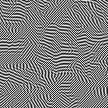
Figure 3: A solution of Eq. 19 for $\tilde{\varepsilon}=0.12$. This is a $512\times 512$ ($\Gamma^{*}=150$) cutout from the center of a $1024\times 1024$ image with $\Gamma^{*}=300$. A movie is available MOV2 .

The finite size of the pattern images has a significant impact on the accuracy of a measurement of $\xi$ from $S\left(k\right)$. To study this effect, we ran simulations using the Swift-Hohenberg model for domain chaos CMT . We utilized the algorithm in Ref. CMT and periodic boundary conditions to solve the equation

$$\partial_{t}\psi=\tilde{\varepsilon}\psi-\left(\nabla^{2}+1\right)^{2}\psi-g_{1}\psi^{3}+g_{2}\hat{z}\cdot\nabla\times\left[\left(\nabla\psi\right)^{2}\nabla\psi\right]+g_{3}\nabla\cdot\left[\left(\nabla\psi\right)^{2}\nabla\psi\right]$$ (19)

for $\psi$, a field that can be used to model the temperature of the convection sample at the midplane. Figure 3 shows an example of $\psi$. The time step for numerical integration was $0.1$. The initial condition for $\psi$ was a random grid of straight-roll patches. At each $\tilde{\varepsilon}$, $10000$ warmup time steps were performed followed by $256$ snapshots of $\psi$ recorded at an interval of $1250$ time steps. The pixel spacing was chosen to reflect a non-unity sample thickness, unlike the choice in Ref. CMT , in order for the wave number and $\xi$ to be nearer the values in the experiment. The choice of this constant has no effect on the value of $\nu$, $\beta$, or $\mu$, thus it does not affect our main conclusions.

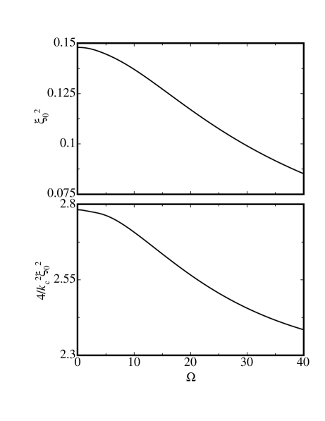
Figure 4: Top figure: curvature $\xi_{0}^{2}$ of the neutral curve. Bottom figure: $4/k_{c}^{2}\xi_{0}^{2}$.

The control parameter in the simulation is related to the experimental control parameter by $\tilde{\varepsilon}=\left(4/k_{c}^{2}\xi_{0}^{2}\right)\varepsilon=2.60\varepsilon$ CH93 , where $k_{c}$ is the critical wave number and $\xi_{0}$ is the curvature of the neutral curve SCEQ . The numerical value $2.60$ corresponds to $\Omega=17.5$. Figure 4 shows both $\xi_{0}^{2}$ and $4/k_{c}^{2}\xi_{0}^{2}$ as a function of $\Omega$ as computed numerically from the neutral curve. We note that the exact value of $4/k_{c}^{2}\xi_{0}^{2}$ has no effect on the results for $\xi$, $B$, $\nu$, $\beta$, $f$, or $\mu$, and only serves to adjust the range of $\varepsilon$.

The parameters $g_{1}$, $g_{2}$, and $g_{3}$ control the stability balloon and can be chosen to model a specific $\Omega$ and Küppers-Lortz angle $\theta_{KL}$. In the present work we used $g_{1}=1$, $g_{2}=-2.4534$, and $g_{3}=0.522$ which are the same parameters used in Fig. 1b of Ref. CMT and which correspond to $\theta_{KL}=51^{\circ}$ and roughly $\Omega\simeq 17.5$ for the Prandtl number in the present experiment. Note that Eq. 19 assumes infinite Prandtl number, so this rough value of $\Omega$ comes from comparing $\Omega/\Omega_{c}$, where $\Omega_{c}$ is Prandtl number dependent.

As a check on the accuracy of our implementation of the solver algorithm we attempted to reproduce Fig. 7a of Ref. CMT . Our simulation agreed within 2% for the data points at $\tilde{\varepsilon}=0.1$, $0.2$, and $0.3$ in that figure, but differed by about 27% for the data point at $\tilde{\varepsilon}=0.03$ for an unknown reason. Nevertheless, we are confident in the correctness of our simulation and in the results to follow.

In order to determine the effect of the finite image size on the measured value of $\xi$ we ran simulations of image size $1024\times 1024$ corresponding to an image aspect ratio $\Gamma^{*}=300$, where $\Gamma^{*}$ refers to the horizontal width of the image. This is in contrast to the aspect ratio $\Gamma$ which refers to the physical aspect ratio of the convection sample. From these large simulations we cut various sized center sections and computed the SF using both the FT and the MEM following the procedure described in Sect. III. We fit the SH function and the squared SH function to the SF.

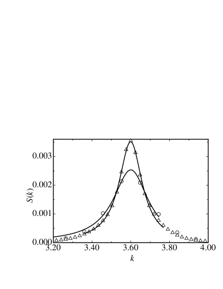
Figure 5: Structure factor (SF) from simulations using Eq. 19 with $\tilde{\varepsilon}=0.12$, computed with the Fourier-transform method. Both data sets are from the same simulation except with a different size center-cutout used to compute the SF. Triangles: $\Gamma^{*}=300$. Circles: $\Gamma^{*}=75$. Solid lines: Fits of Eq. 1 to the data over the range $k\pm 3/\xi$.

The choice of $\Gamma^{*}$ strongly affected the shape of the SF when computed with the FT. Figure 5 compares the SF of the same data for two different values of $\Gamma^{*}$. The same data analyzed with the MEM, as shown in Fig. 6, is affected slightly by $\Gamma^{*}$, but it is not nearly as sensitive as the FT. It is important to note that the sharpest SF peak is not necessarily the best. The $\Gamma^{*}=300$ SF from the FT is sharper than either of the MEM peaks, but it is not at all consistent with its shorter data length relative, $\Gamma^{*}=75$. In contrast, the MEM SFs land nearly on top of each other when comparing $\Gamma^{*}=300$ and $\Gamma^{*}=75$. The ability to accurately represent the SF peak for relatively small image sizes is crucial because system sizes as large as $\Gamma^{*}=300$ are experimentally inaccessible.

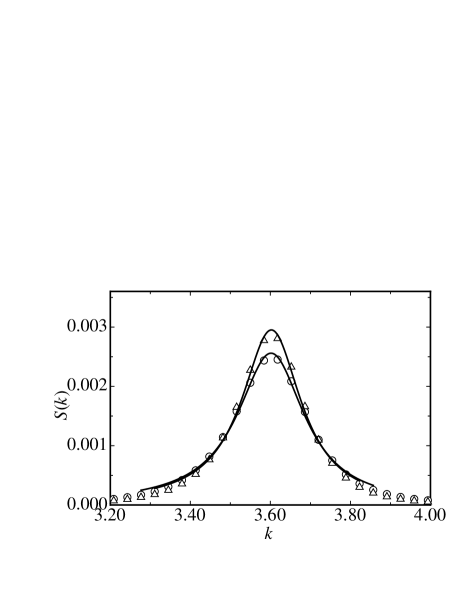
Figure 6: Structure factor (SF) from simulations using Eq. 19 with $\tilde{\varepsilon}=0.12$, computed with the maximum entropy method (MEM). Both data sets are from the same simulation except with a different size center-cutout used to compute the SF. Triangles: $\Gamma^{*}=300$. Circles: $\Gamma^{*}=75$. Solid lines: Fits of Eq. 1 to the data over the range $k\pm 3/\xi$.

From fitting the SF for both the FT and MEM, we computed $\xi$ for many $\varepsilon$ and $\Gamma^{*}$ as shown in Fig. 7. Once again we found that the MEM provides significantly more consistent results for vastly different $\Gamma^{*}$. In the case of the FT results, it is critical to note that increasing $\Gamma^{*}$ does not simply increase $\xi$ due to the larger data length. It also increases the slope of $\xi$ vs. $\varepsilon$ on logarithmic scales, thus affecting the measured $\nu$. Since we wish to measure $\nu$ accurately enough to compare with the model prediction $\nu=1/2$, this is a discouraging outcome.

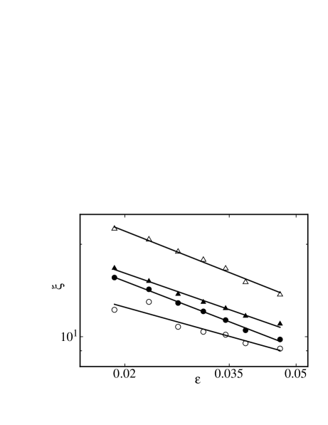
Figure 7: Measurements of $\xi$ from fits of Eq. 1 to many SFs like those shown in Figs. 5 and 6. Open symbols: from the FT method. Solid symbols: from the MEM. Triangles: $\Gamma^{*}=300$. Circles: $\Gamma^{*}=75$. Solid lines: Fits of the power law $\xi\propto\varepsilon^{-\nu}$ to the data over the range shown.

We ascertained the effect of image size on the accuracy of $\nu$ by computing $\nu$ as a function of $\Gamma^{*}$ as shown in Fig. 8. The two lowest $\Gamma^{*}$ points in that figure correspond to the available image size in the experimental samples discussed in the present work. The $\nu$ values from the MEM and FT method both approached nearly the same asymptotic value at large $\Gamma^{*}$. Fortunately, the result from the MEM has nearly reached this asymptote at even the smallest $\Gamma^{*}$ indicating that it may be reliably used for measuring $\nu$ even in the case of small images. Not only is the FT measurement of $\nu$ much too low at the smallest $\Gamma^{*}$, but it also contains rather large fluctuations at those values. At the largest $\Gamma^{*}$ it is almost as good as the MEM, but that does not help for the analysis of experiments which are limited roughly to $\Gamma^{*}<100$ BSCA05 .

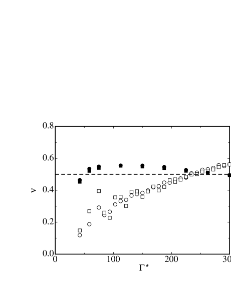
Figure 8: Results for $\nu$ from fits like those shown in Fig. 7. Solid symbols: from the MEM. Open symbols: from the FT method. Circles: $\xi$ was determined by fitting the SH SF Eq. 1 to the data. Squares: $\xi$ was determined by fitting a squared SH SF Eq. 2 to the data. Dashed line: the $\nu=1/2$ prediction from model equations.

We observed a similar finite image-size effect for the scaling of $B$ with $\varepsilon$. As discussed in Sect. II we expect that $B\sim\varepsilon^{1/2}$ provided that $\xi$ obeys the scaling in the amplitude model, i.e. $\xi\sim\varepsilon^{-1/2}$. Our SF fits that yielded $\xi$ also gave $B$. Figure 9 shows some examples of $B$ for the same data as shown in Fig 7.

Figure 9: Results for $B$ from fits of Eq. 1 to many SFs like those shown in Figs. 5 and 6. Open symbols: from the FT method. Solid symbols: from the MEM. Triangles: $\Gamma^{*}=300$. Circles: $\Gamma^{*}=75$. Solid lines: Fits of the power law $B\propto\varepsilon^{\beta}$ to the data over the same range as shown in Fig. 7.

We extracted a scaling exponent $\beta$ by fitting the equation $B\propto\varepsilon^{\beta}$ to the data. As indicated by Fig. 10, the result is similar to the finite image-size effect on $\nu$. At the smallest $\Gamma^{*}$ values, the MEM results exhibit a slight $\Gamma^{*}$ dependence, but they quickly reach a nearly constant value as $\Gamma^{*}$ increases. The FT method suffers from a strong $\Gamma^{*}$ dependence. However, it is quite satisfying that for $\Gamma^{*}$ near the experimental values, we obtained $\nu\simeq 0.25$ and $\beta\simeq 0.75$ from the FT method, in agreement with what we (and others previously) observed in the experiment.

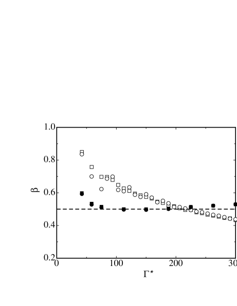
Figure 10: Results for $\beta$ from fits like those shown in Fig. 9. Solid symbols: from the MEM. Open symbols: from the FT method. Circles: $\xi$ was determined by fitting the SH SF Eq. 1 to the data. Squares: $\xi$ was determined by fitting the squared SH SF Eq. 2 to the data. Dashed line: the $\beta=1/2$ prediction from model equations.

Figure 11 shows the results for $\nu+\beta$ for both the MEM and the FT method. Both are close to the expected result $\nu+\beta=1$, and approach it even more closely as $\Gamma^{*}$ increases.

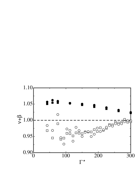
Figure 11: Values of $\nu+\beta$ from combining the results shown in Figs. 8 and 10. Solid symbols: from the MEM. Open symbols: from the FT method. Circles: $\xi$ and $B$ determined by fitting the SH SF Eq. 1 to the SFs. Squares: $\xi$ and $B$ determined by fitting the squared SH SF Eq. 2 to the SFs. Dashed line: $\nu+\beta=1$.

Unlike for $\xi$ and $B$, the finite image size does not interfere with the determination of the characteristic frequency scale $f$ of the domain chaos (the domain precession frequency) when the FT method is used to compute the SF. We computed $f$ using the method explained in Ref. HPAE98 . We extracted a time scale from the auto-correlation of the angle-time plot of the radially averaged SF. This yielded the results for $f$ shown in Fig. 12. All of the $f$ data in that figure land nearly on top of each other regardless of $\Gamma^{*}$. Since the measurement of $f$ depends more on the position of the peak in the two-dimensional SF than on its width, the FT method is able provide enough resolution to accurately measure $f$ at smaller $\Gamma^{*}$.

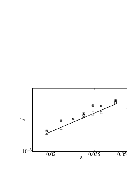
Figure 12: Determinations of the characteristic frequency scale $f$ of the domain chaos from the auto-correlations of time-angle plots of the SFs computed with the FT method. Triangles: $\Gamma^{*}=300$. Squares: $\Gamma^{*}=150$. Circles: $\Gamma^{*}=75$. Crosses: $\Gamma^{*}=58.6$. Pluses: $\Gamma^{*}=42.2$. Solid line: Fit of the power law $f\propto\varepsilon^{\mu}$ to the data over the same range as shown in Fig. 7.

We fit a power law $f\propto\varepsilon^{\mu}$ to $f$ because the GL model predicts such a power law with $\mu=1$. Figure 13 shows that this exponent is independent of $\Gamma^{*}$. However, the result $\mu\simeq 0.9$ is somewhat lower that the predicted value. We do not know the reason for this. However, the value we found for $\mu$ is much larger than the experimental value $\mu\simeq 0.6$ HEA1 . Recently it was found BSCA05 that this difference is caused by the centrifugal force which influences the experiment but is omitted in Eq. 19.

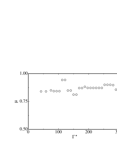
Figure 13: Measurements of $\mu$ from fits, like those shown in Fig. 12, to data for $f$ computed from SFs with the FT method.

V New experimental measurements

We acquired new data using an apparatus described previously BBMTHCA96 . There were two samples which both used compressed SF₆ gas. The primary sample was at a pressure of 20.00 bars and mean temperature of $38.00^{\circ}\textrm{C}$ where the Prandtl number $\eta/\left(\rho\kappa\right)$ ($\kappa$ is the thermal diffusivity) was $0.87$. The aspect ratio $\Gamma\equiv D/\left(2d\right)$ ($D$ is the sample diameter) was 61.5. A secondary sample with $\Gamma=36$, which is discussed briefly in this work, was pressurized at 12.34 bars with a mean temperature of $38.00^{\circ}\textrm{C}$ and the Prandtl number was $0.82$.

We determined $\xi$ by fitting each of the functions in Eqs. 1-4, multiplied by the shadowgraph transfer function from Refs. BBMTHCA96 ; TC03 , to the data near the peak of the SF. Typically we used a range $k_{0}\pm 3/\xi$ where the initial guess of $\xi$ and $k_{0}$ for the fitting range was estimated by Eq. 6 using the zeroth numerical moment, peak value, and peak position. The fit was not very sensitive to the range of $k$ provided that the range included a sufficient number of points. Figure 14 shows that for the FT method, all of the functions provide a good fit near the half height, where $\xi$ is determined, and near the peak where the fits give the value of $B$. Figure 15 shows similarly good fitting results for the SF estimated with the MEM.

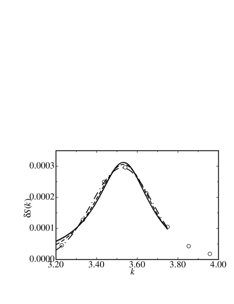
Figure 14: Fits of Eqns. 1-4 to the experimental SF computed with the FT for $\Omega=17.7$ and $\varepsilon=0.05$. Solid line: fit of SH SF Eq. 1. Dashed line: fit of squared SH SF Eq. 2. Dashed-dotted line: fit of Gaussian SF Eq. 3. Dotted line: fit of Lorentzian SF Eq. 4. All fitting functions are multiplied by the shadowgraph transfer function.

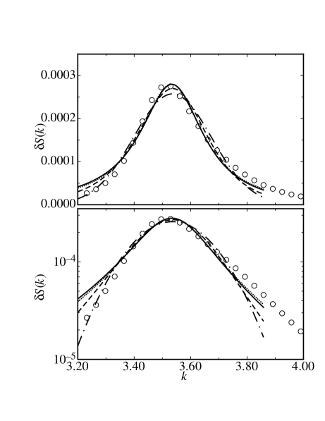
Figure 15: Fits of Eqns. 1-4 to the experimental SF computed with the MEM for $\Omega=17.7$ and $\varepsilon=0.05$. Top figure: linear-linear plot. Bottom figure: log-linear plot. Solid line: fit of SH SF Eq. 1. Dashed line: fit of squared SH SF Eq. 2. Dashed-dotted line: fit of Gaussian SF Eq. 3. Dotted line: fit of Lorentzian SF Eq. 4. All fitting functions are multiplied by the shadowgraph transfer function.

Figure 16 shows the effect of the fitting function on the dependence of $\xi$ on $\varepsilon$ for $\Omega=17.7$. Although each of the fitting functions gave slightly different values for $\xi$, all of them gave nearly the same value for $\nu$, with $\nu\simeq 0.25$ from the FT method and $\nu\simeq 0.5$ from the MEM. This suggests that the function fitting is a robust method for measuring $\xi$ because knowledge of the exact functional form of the SF is not required to yield a consistent measurement for $\xi$. In spite of this consistency for $\nu$, we concluded that some fitting functions are better than others as will be seen below.

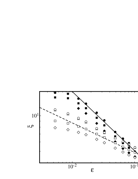
Figure 16: Measurements of $\xi$ by fitting Eqns. 1-4 to the experimental SF for $\Omega=17.7$. Open symbols: SF was computed using a Kaiser-Bessel window with $\alpha=2.5$. Solid symbols: SF was computed with the MEM. Dashed line: $\varepsilon^{-1/4}$. Solid line: $\varepsilon^{-1/2}$. Circles: $\xi$ from fitting of SH SF. Squares: $\xi$ from fitting of squared SH SF. Diamonds: $\xi$ from fitting of Gaussian SF. Triangles: $\xi$ from fitting of Lorentzian SF.

The results from the MEM are in much better agreement, than the results from the FT method, with the prediction $\nu=1/2$ from the GL model. This difference is even more dramatic when considering a smaller-sized cutout region from the data. Figure 17 shows $\xi$ for two different $\Gamma$, where the analysis has been applied to a central region of identical size in either case. Although in the case of $\Gamma=61.5$ the data shown in Fig. 17 is from the same raw data as shown in Fig. 16, the FT method gives a somewhat smaller value of $\nu$ because of the reduced image size of the smaller cutout region. The MEM also suffers some minor decrease in the value of $\nu$, as this cutout size corresponds to the smallest $\Gamma^{*}$ data point in Fig. 8. Although only barely noticeable in the FT result, the MEM clearly shows that $\xi$ is larger in the case of $\Gamma=36$ as compared to $\Gamma=61.5$. A likely explanation is the increased influence of the centrifugal force in the larger sample. The presence of the centrifugal force has been shown to decrease the domain size BSCA05 .

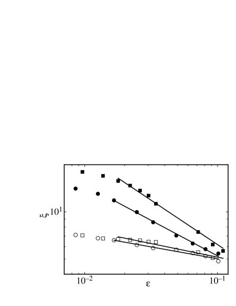
Figure 17: Comparison of $\xi$ for $\Omega=17.7$ and both $\Gamma=36$ and $\Gamma=61.5$, measured with SFs computed from $44d\times 44d$ square cutouts using both the MEM and the FT method. Squares: $\Gamma=36$. Circles: $\Gamma=61.5$. Open symbols: FT. Solid symbols: MEM. For $\Gamma=36$ the fitting range was $0.018\leq\varepsilon\leq 0.11$, MEM: $\nu=0.57$, FT: $\nu=0.17$. For $\Gamma=61.5$ the fitting range was $0.017\leq\varepsilon\leq 0.10$, MEM: $\nu=0.45$, FT: $\nu=0.15$.

The diminishing slope at very small $\varepsilon$ shown in Figs. 16 and 17 may be indicative of a physical finite-size effect CLM01 due to the lateral boundary of the experimental samples. However, over the range of fitting shown in Fig. 17, no such effect is observed. As a comparison with the result in Fig. 3 of Ref. CLM01 , Fig. 18 shows a plot of $\varepsilon^{-1/2}$ scaled with $\xi$ against $\varepsilon^{-1/2}$ scaled with $\Gamma$. The data is roughly constant over the range of $\varepsilon$ indicating agreement with the GL prediction for $\nu$. Unfortunately the data from two different $\Gamma$ do not collapse onto a single curve as in Ref. CLM01 . This may be due to the effect of the centrifugal force, which was neglected in that work, but is unavoidable in the present experiment.

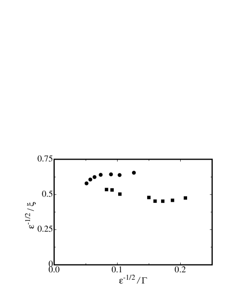
Figure 18: $\varepsilon^{-1/2}$ scaled against $\xi$ and $\Gamma$ for $\Omega=17.7$ and both $\Gamma=36$ and $\Gamma=61.5$, measured with SFs computed from $44d\times 44d$ square cutouts using the MEM. Squares: $\Gamma=36$. Circles: $\Gamma=61.5$. The data is the same as in Fig. 17 and is shown over the range of the fits in that figure.

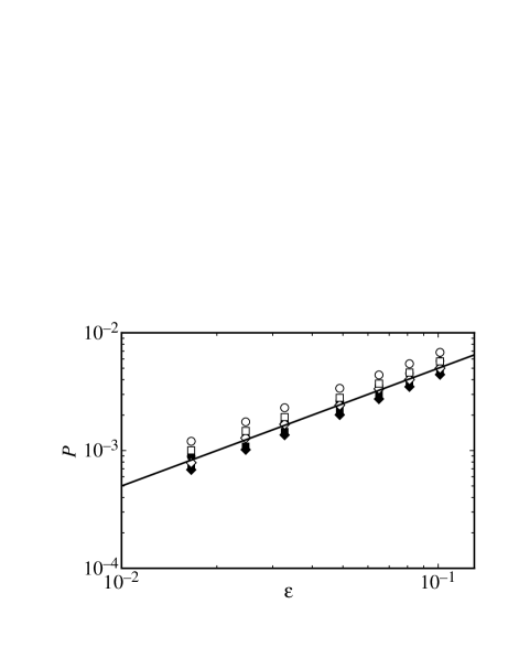
Figure 19: Total power for $\Omega=17.7$ from SFs computed with both the FT method and the MEM and given by various methods. Solid line: $\varepsilon^{1}$. Open symbols: from the FT method. Solid symbols: from the MEM. Diamonds: power from zeroth numerical moment of the SF data integrated over $k_{0}-3/\xi\leq k\leq k_{0}+3/\xi$. Circles: power given by Eq. 5 using the parameters acquired from fitting the SH SF to the data. Squares: power given by Eq. 7 using the parameters acquired from fitting the squared SH SF to the data.

Although, in the case of the FT method, the scaling exponent $\nu$ did not agree with the GL model, the scaling of the total power agreed for both the FT method and the MEM. Figure 19 shows the total power for $\Omega=17.7$ measured by several methods. The zeroth numerical moment of the data did not perfectly agree with the total power computed from Eq. 5 or Eq. 7 but it was close. In the case of those equations, the fit parameters $B$, $k_{0}$, and $\xi$ (or $\xi_{s}$ for the squared SH) were used to calculate $P$. Since Eqs. 5 and 7 represent the total power over the range $0<k<\infty$ and the zeroth numerical moment was necessarily computed over a finite range $k_{0}-3/\xi\leq k\leq k_{0}+3/\xi$, the slight discrepancy in total power is not surprising. A numerical integration of Eqs. 1 and 2 over a finite $k$ range yields a total power closer to the numerical moment result, however, it is absent from Fig. 19 because it is too close to the other data points to be easily distinguishable. In spite of this minor discrepancy, all three measurements of the total power are proportional to $\varepsilon$ as expected.

Since, in the case of the FT method, the dependence of $\xi$ on $\varepsilon$ differed from the GL prediction of $\varepsilon^{-1/2}$, it is important to also investigate the dependence of $B$ on $\varepsilon$. As shown in Fig. 19, the combination of $B$ and $\xi$ according to Eqs. 6 and 8 yielded a total power that depended on $\varepsilon$ in the predicted way for both the FT method and the MEM.

Figure 20 shows the result for $B$ measured by fitting the SH SF to the experimental SF at all $\Omega$ values. The slight variation of the values of $\beta$ (slopes of the lines in the figure) did not depend systematically on $\Omega$ and most likely it is due to experimental error. The power-law fits shown in the figure were over the same range as was used to determine $\nu$ in Fig. 21. One sees that $B$ alone did not depend on $\varepsilon^{1/2}$ as expected; instead $B\sim\varepsilon^{\beta}$ with, averaging over the results from all $\Omega$, $\beta\simeq 0.73$ while the $\Omega$-averaged $\nu\simeq 0.25$. In other words, in the case of the FT method, $B$ and $\xi$ conspired to produce the expected $P\sim\varepsilon^{\nu+\beta}$ with $\nu+\beta\simeq 1$.

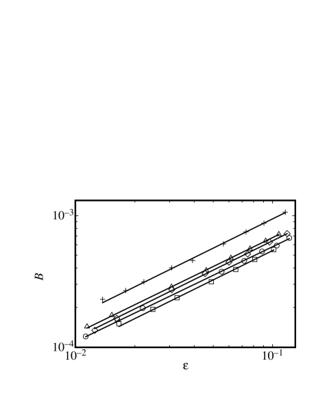
Figure 20: $B$ determined by fitting the FT experimental SF to the SH function. Solid lines: power law fits to the data to measure $\beta$. Pluses: $\Omega=15$. Circles: $\Omega=16.25$. Squares: $\Omega=17.7$. Triangles: $\Omega=19.5$. Diamonds: $\Omega=21.7$.

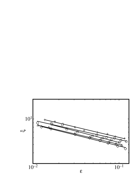
Figure 21: $\xi$ determined by fitting the FT experimental SF to the SH function. Solid lines: power-law fits to the data to determine $\nu$. Pluses: $\Omega=15$. Circles: $\Omega=16.25$. Squares: $\Omega=17.7$. Triangles: $\Omega=19.5$. Diamonds: $\Omega=21.7$.

Figures 22 and 23 show the analogous results from the MEM. The MEM yielded much more steeply sloped $\xi$ vs. $\varepsilon$ curves as indicated by Fig. 23. The resulting $\nu$ was in much better agreement with the GL model prediction. Likewise, $\beta$ was much closer to $1/2$ than for the FT method. Averaged over $\Omega$, $\nu\simeq 0.46$ and $\beta\simeq 0.63$ from the MEM. Figure 24 summarizes the behavior of the exponents for both the MEM and the FT method as a function of $\Omega$. The MEM clearly gave the closest result in agreement with the prediction $\nu=1/2$ and also $\beta=1/2$. However, the FT method yielded the best agreement with the prediction $\nu+\beta=1$, with the MEM not much further off. Considering the results of Sect. IV, the MEM is more reliable. Thus we conclude that the experimental length scale is in agreement with the prediction from the GL model.

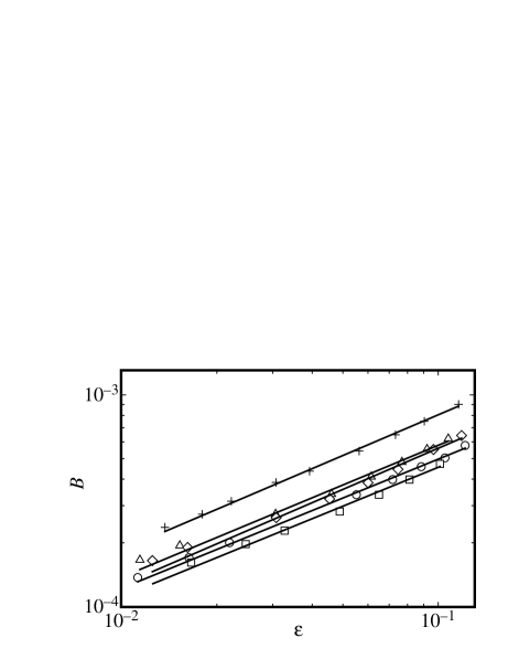
Figure 22: $B$ determined by fitting the MEM experimental SF to the SH function. Solid lines: power-law fits to the data to determine $\beta$. Pluses: $\Omega=15$. Circles: $\Omega=16.25$. Squares: $\Omega=17.7$. Triangles: $\Omega=19.5$. Diamonds: $\Omega=21.7$.

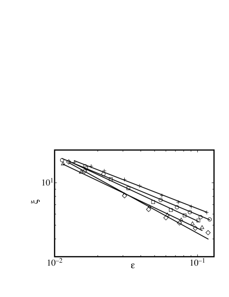
Figure 23: $\xi$ determined by fitting the MEM experimental SF to the SH function. Solid lines: power-law fits to the data to determine $\nu$. Pluses: $\Omega=15$. Circles: $\Omega=16.25$. Squares: $\Omega=17.7$. Triangles: $\Omega=19.5$. Diamonds: $\Omega=21.7$.

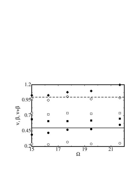
Figure 24: Exponents from data shown in Figs. 20-23. Open symbols: from the FT method. Solid symbols: from the MEM. Circles: $\nu$. Squares: $\beta$. Diamonds: $\nu+\beta$. Solid line: $\nu=\beta=1/2$ prediction from GL model. Dashed line: $\nu+\beta=1$.

VI Scaling of $\delta S\left(k\right)$ for Experimental Data and Analytic Functions

The scaling analogy to critical phenomena extends beyond the power-law dependence of $\xi$ and $B$ on $\varepsilon$. In order to more deeply probe this scaling, we re-scaled the SFs at different $\varepsilon$ in an attempt to collapsed them all onto a single curve. We followed the procedure of Ref. XLG97 . First we normalized the structure factor so that $2\pi$$\int_{0}^{\infty}\delta S\left(k\right)kdk=1$. In applying this normalization to the experimental data, we evaluated the integral over the range $k_{0}-3/\xi\leq k\leq k_{0}+3/\xi$. This included most of the total power present in the experimental data. Figure 25 shows the MEM results for several $\varepsilon$ values and demonstrates that normalization alone is not sufficient to collapse the data onto a unique curve. It is also necessary to re-scale the SF on both the abscissa and ordinate axes so that $x\equiv\left(k-k_{0}\right)\xi$ and $\delta\tilde{S}\left(x\right)\equiv\left(k/\xi\right)\delta S\left(x\right)$.

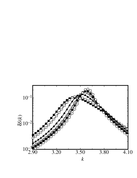
Figure 25: The normalized SFs for $\Omega=17.7$ computed with the MEM. Open circles: $\varepsilon=0.017$. Solid circles: $\varepsilon=0.025$. Open triangles: $\varepsilon=0.033$. Solid triangles: $\varepsilon=0.05$. Open squares: $\varepsilon=0.08$. Solid squares: $\varepsilon=0.10$.

Applying this variable transformation to the analytic forms in Eqs. 1-4 provides some insight into the effect of rescaling. In the critical-point limit, of $\xi\rightarrow\infty$ and evaluating the integral normalization over the range $0\leq k\leq\infty$, all parameters cancel, leaving only a function of $x$. This yields

$$\tilde{S}\left(x\right)=\frac{1}{2\pi^{2}\left(1+x^{2}\right)}$$ (20)

in the case of the SH form,

$$\tilde{S}\left(x\right)=\frac{1}{\pi^{2}\left(1+x^{2}\right)^{2}}$$ (21)

in the case of the squared SH form, and

$$\tilde{S}\left(x\right)=\frac{\exp\left(-x^{2}\right)}{2\pi^{3/2}}$$ (22)

in the case of the Gaussian form. We refrain from listing the rescaled Lorentzian because the zeroth moment diverges, making it impossible to normalize without introducing a cutoff.

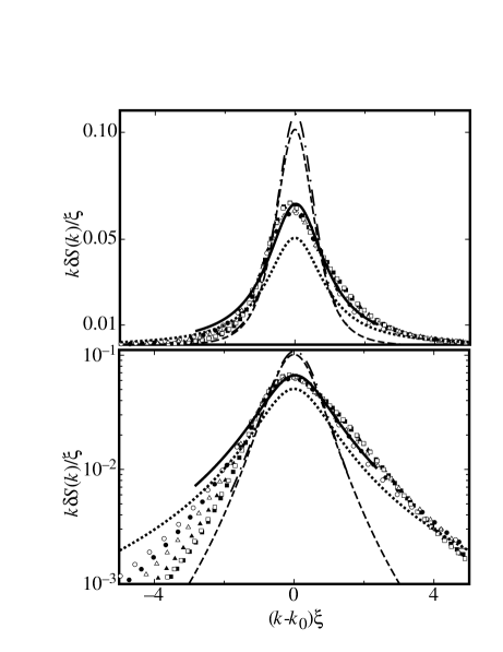
Figure 26: Scaled SFs for $\Omega=17.7$ computed with the MEM. Top figure: linear-linear plot. Bottom figure: log-linear plot. The symbols are as in Fig. 25. Dotted line: rescaled SH SF Eq. 20. Dashed line: rescaled squared SH SF Eq. 21. Solid line: numerically rescaled SH SF using finite limits for its normalization. Dashed-dotted line: numerically rescaled squared SH SF using finite limits for its normalization.

Figure 26 shows the re-scaled experimental SFs from the MEM on a linear (top figure) and on a logarithmic (bottom figure) scale. Although not shown, we found comparable results for both the normalized and rescaled SFs computed with the FT method. The figure also includes the rescaled SH and squared SH SFs given by Eqs. 20 and 21. We omit the Gaussian form in Eq. 22 in order to maximize the clarity of the figure. It is the poorest empirical representation out of Eqs. 20-22, and the least physically justifiable. Note that the curves of Eqs. 20 and 21 are not fits to the experimental data; there are no free parameters for fitting. None of them provide a particularly good scaled representation of the data near the peak. The experimental results fall somewhere between the SH (dotted line) and the squared SH (dashed line) form.

The disagreement between the scaled data and the scaled functions is primarily due to the normalization of the experimental data, which is over a finite range unlike the normalization in Eqs. 20 and 21 which is over all $k$. Also shown are collapsed forms of Eqs. 1 and 2 computed numerically using the normalization over the same finite range as in the experimental SFs. The numerically-computed forms were evaluated at finite $\varepsilon$, instead of taking the limit of $\xi\rightarrow\infty$, as was done in the analytic cases of Eqs. 20-22. As a result, $\xi$ and $k_{0}$ remained as constants in the collapsed forms. We used the values of $\xi$ and $k_{0}$ from the $\varepsilon=0.10$ data point. This choice barely affected the numerically collapsed curves because $k_{0}\xi$ was relatively large for all values of $\varepsilon$ shown. These curves provide insight into the agreement of the shape of Eqs. 1 and 2 with the experimental data. The numerically computed SH SF agreed quite well with the collapsed experimental data, while the squared SH SF did not.

VII Summary and Conclusion

In this paper we carefully examined two methods, the FT method and the MEM NR , for determining critical parameters describing the spatio-temporal chaos state in rotating Rayleigh-Bénard convection known as domain chaos. We found that a correlation length $\xi$, equal to the inverse half-width at half-height of the structure factor $S(k)$, can be determined reliably by fitting one of several trial functions to the experimental data. We examined a Lorentzian, Swift-Hohenberg, squared Swift-Hohenberg, and Gaussian form. We prefer this fitting method over computing numerical moments from the data (as had been done in the past) because we were able to show analytically that the length $\bar{\xi}=1/\sigma$ ($\sigma^{2}$ is the variance of the data) will be proportional to $\xi$ only when $S(k)$ decreases sufficiently fast at large $k$.

For a technique of estimating the SF, we found that the MEM was much superior to the classic FT method. There is a severe dependence on image size in the case of the FT method that is quite apparent from our analysis of various sized images from the simulation using the SH domain-chaos model. Since the experimental images are relatively small, the MEM is required in order to accurately determine the SF from the patterns.

We analyzed new experimental shadowgraph images of domain chaos for a sample of aspect ratio $\Gamma=61.5$ over the range $15\stackrel{{\scriptstyle<}}{{{}_{\sim}}}\Omega\stackrel{{\scriptstyle<}}{{{}_{\sim}}}22$. Using the above four functional forms as fitting functions, we obtained results for $\xi$ that depended only slightly on the function used, but that all had the same dependence on the distance $\varepsilon$ from the onset of convection. In the case of the FT method, we found $\xi\sim\varepsilon^{-\nu}$ with $\nu\simeq 0.25$, in agreement with previous measurements for a sample with $\Gamma=40$ but in disagreement with expectations based on the weakly-nonlinear amplitude model. Fortunately the MEM was able to overcome the image-size problem of the FT method and yielded $\nu\simeq 0.46$, roughly in agreement with the theoretical models. We also determined the maximum height $B$ of $S(k)$ from fits of the functions to the data and found that $B\sim\varepsilon^{\beta}$ with $\beta\simeq 0.73$ for the FT method, in disagreement with the value $\beta=1/2$ suggested by the amplitude model. However, we note that the FT method yielded a total power proportional to $\varepsilon^{\nu+\beta}$ with $\nu+\beta\simeq 0.98$, that agrees with the theoretical expectation that $\nu+\beta=1$. The MEM yielded $\beta\simeq 0.63$, somewhat closer to the prediction of $\beta=1/2$ than the FT method.

We also showed that it is possible to present the structure factor in a scaled form that largely collapses the data onto a unique curve. This was the case for both the FT method and the MEM, even though the scaling exponents of the FT method results did not agree with the prediction from theory.

In summary, our new experimental data and analysis yielded results that differ from the earlier result that $\nu\simeq 0.25$ in disagreement with theory. We have shown that this difference is due to the limitations of the FT analysis method. The MEM is capable of extracting scaling exponents from the data that are in agreement with the theoretical prediction. In addition to the exponent $\nu$, we also examined a scaling parameter $\beta$ that describes the height of the structure factor, and found it to also agree with predictions when the MEM results were used.

VIII Acknowledgment

We are grateful for numerous stimulating conversations with a number of people, including especially E. Bodenschatz, M.C. Cross, P.C. Hohenberg, M. Paul, W. Pesch, and J.D. Scheel. This work was supported by the US National Science Foundation through Grant DMR02-43336.

References

- (1) See, for instance, M.C. Cross and P.C. Hohenberg, Rev. Mod. Phys. 65, 851 (1993).
- (2) For a review, see for instance E. Bodenschatz, W. Pesch, and G. Ahlers, Annu. Rev. Fluid Mech. 32, 709 (2000).
- (3) S. Chandrasekhar, Hydrodynamic and Hydromagnetic Stability, (Oxford University Press, Oxford, 1961).
- (4) G. Küppers and D. Lortz, J. Fluid Mech. 35, 609 (1969).
- (5) G. Küppers, Phys. Lett. 32A, 7 (1970).
- (6) R.M. Clever and F.H. Busse, J. Fluid Mech. 94, 609 (1979).
- (7) K.E. Heikes and F.H. Busse, Ann. N.Y. Acad. Sci. 357, 28 (1980).
- (8) F.H. Busse and K.E. Heikes, Science 208, 173 (1980).
- (9) Y.-C. Hu, R. Ecke, and G. Ahlers, Phys. Rev. Lett. 74, 5040 (1995).
- (10) Y.-C. Hu, R. Ecke, and G. Ahlers, Phys. Rev. E 55, 6928 (1997).
- (11) Y. Hu, W. Pesch, G. Ahlers, and R.E. Ecke, Phys. Rev. E 58, 5821(1998).
- (12) See EPAPS Document No. ??? for an MPEG movie of Fig. 1a at actual speed. This document can be reached via a direct link in the online article’s HTML reference section or via the EPAPS homepage (http://www.aip.org/pubservs/epaps.html).
- (13) J.M. Rodriguez, C. Perez-Garcia, M. Bestehorn, M. Fantz, and R. Friedrich, Phys. Rev. A 46, 4729 (1992).
- (14) M. Fantz, R. Friedrich, M. Bestehorn, and H. Haken, Physica D 61, 147 (1992).
- (15) M. Neufeld, R. Friedrich, and H. Haken, Z. Phys. B 92, 243 (1993).
- (16) Y. Tu and M. Cross, Phys. Rev. Lett. 69, 2515 (1992).
- (17) M. Cross, D. Meiron, and Y. Tu, Chaos 4, 607 (1994).
- (18) Y. Ponty, T. Passot, and P. Sulem, Phys. Rev. Lett. 79, 71 (1997).
- (19) Y. Ponty, T. Passot, and P. Sulem, Phys. Rev. E 56, 4162 (1997).
- (20) D. Laveder, T. Passot, Y. Ponty, and P. L. Sulem, Phys. Rev. E 59, R4745 (1999).
- (21) K.M.S. Bajaj, N. Mukolobwiez, N. Currier, and G. Ahlers, Phys. Rev. Lett. 83, 5282 (1999).
- (22) K.M.S. Bajaj, N. Mukolobwiez, J. Oh, and G. Ahlers, J. Stat. Mech., submitted.
- (23) M. C. Cross, M. Louie, and D. Meiron, Phys. Rev. E 63, 45201 (2001).
- (24) S. W. Morris, E. Bodenschatz, D. S. Cannell, and G. Ahlers, Phys. Rev. Lett. 71, 2026 (1993).
- (25) We distinguish between finite-sample-size effects due to the lateral boundaries that were discussed in Ref. CLM01 , and finite image-size effects that would prevail even if a small image were extracted from a central region of a much larger sample.
- (26) J. M. Ortiz de Zárate and J. V. Sengers, Phys. Rev. E 66, 036305 (2002).
- (27) M.C. Cross and D.I. Meiron, Phys. Rev. Lett. 75, 2152 (1995).
- (28) Q. Hou, S. Sasa, and N. Goldenfeld, Physica A 239, 219 (1997).
- (29) J. F. Kaiser, in System Analysis by Digital Computer, edited by F. F. Kuo and J. F. Kaiser (John Wiley & Sons, Inc., New York, 1966), p. 232.
- (30) M. Frigo and S. G. Johnson, in Proc. 1998 IEEE Intl. Conf. Acoustics Speech and Signal Processing, (IEEE, 1998), p 1381.
- (31) Y.-C. Hu, Ph.D. Thesis, University of California at Santa Barbara, 1995 (unpublished).
- (32) M. Wu, G. Ahlers, and D.S. Cannell, Phys. Rev. Lett. 75, 1743 (1995).
- (33) J. Oh and G. Ahlers, Phys. Rev. Lett. 91, 094501 (2003).
- (34) W.H. Press, S.A. Teukolsky, W.T. Vetterling, and B.P. Flannery, Numerical Recipes in C, (Cambridge University Press, Cambridge, 1992).
- (35) J.S. Lim, Two-Dimensional Signal and Image Processing, (Prentice-Hall, New Jersey, 1990).
- (36) J.S. Lim and N.A. Malik, IEEE Trans. Acoust., Speech, Signal Processing, 29, 401 (1981).
- (37) N.A. Malik and J.S. Lim, IEEE Trans. Acoust., Speech, Signal Processing, 30, 788 (1982).
- (38) J.R. deBruyn, E. Bodenschatz, S. Morris, S. Trainoff, Y.-C. Hu, D.S. Cannell, and G. Ahlers, Rev. Sci. Instrum. 67, 2043 (1996).
- (39) S.P. Trainoff and D.S. Cannell, Phys. Fluids 14, 1340 (2003).
- (40) See Eq. 159 of Ch. III of Ref. SC for the neutral curve of rotating RBC.
- (41) See EPAPS Document No. ??? for an MPEG movie of a cutout () from Fig. 3 at 1500 time steps per second. This document can be reached via a direct link in the online article’s HTML reference section or via the EPAPS homepage (http://www.aip.org/pubservs/epaps.html).
- (42) N. Becker, J.D. Scheel, M.C. Cross, and G. Ahlers, submitted to Phys. Rev. E.
- (43) H.-W. Xi, X.-J. Li, and J.D. Gunton, Phys. Rev. Lett. 78, 1046 (1997).