Geometry-induced pulse instability in microdesigned catalysts:
the effect of boundary curvature

Abstract

We explore the effect of boundary curvature on the instability of reactive pulses in the catalytic oxidation of CO on microdesigned Pt catalysts. Using ring-shaped domains of various radii, we find that the pulses disappear (decollate from the inert boundary) at a turning point bifurcation, and trace this boundary in both physical and geometrical parameter space. These computations corroborate experimental observations of pulse decollation.

I Introduction

Pattern formation in spatially uniform media has been studied extensively (see e.g. the review by Cross and Hohenberg Cross and Hohenberg (1993) and, specifically for catalytic surfaces, the recent review by Imbihl Imbihl (2005)). Since the pioneering Photoemission Electron Microscopy (PEEM) work of Ertl and coworkers in 1989 Rotermund et al. (1990), high vacuum CO oxidation on single crystal Pt catalysts has been a paradigm for such studies. Current research increasingly focuses on the interplay between spontaneous pattern formation and spatial medium nonuniformity, as well as with spatiotemporal variations of the medium properties. Intentionally designing the geometry of the medium at the microscopic level has been finding an increasing number of applications across disciplines in recent years: from the guidance of cell migration through micropatterning Jiang et al. (2004) and the template-based self-assembly of diblock copolymers (e.g Park et al. (1997)) to the observation of binary fluids Verberg et al. (2004) and phase separation in confined geometries (e.g. Böltau et al. (1998)). Examples of complex, microdesigned geometries used in the study of reacting systems include Belousov-Zhabotinsky (BZ) catalyst microprinting Steinbock et al. (1995) and CO oxidation on microlithographically shaped domains on Pt catalysts Graham et al. (1994). The study of reactive pattern formation in random heterogeneous media is a topic of active current modelling work (e.g. Tusscher and Panfilov (2005); Bub et al. (2005)); natural heterogeneous media (such as water-in-oil microemulsions in Kaminaga et al. (2005)) are also being studied. Microfluidics is another field that hinges on the micron-scale design of geometry to control flow and transport (see e.g. the review Stone et al. (2004)); beyond passive geometry design, extensive developments in active addressing, for example in control of droplet breakup Joanicot and Ajdari (2005) or micromixing Stroock et al. (2002) have been realized. Actively and spatiotemporally altering the activity of chemically reactive media is exemplified in Wolff et al. (2001) for thermally addressed heterogeneous catalytic reactions and in Sakurai et al. (2002) for photosensitive BZ media. The recent work of Lucchetta et al. (2005) marries microfluidic technology with the active addressing of pattern forming reactive media in a developmental biology context, using temperature fields to perturb pattern formation in drosophila embryos.

The interplay of nonlinear reaction-diffusion dynamics with the effects of boundaries has been extensively studied both in theory and in experiments; a remarkable early observation was that rotating spiral waves of a BZ reagent could be initiated close to domain boundaries with sharp corners Agladze et al. (1994). Observations in catalytic reactions include that (a) below a certain critical domain size, the frequency of rotating waves in a small circular domain is affected by the domain size Hartmann et al. (1996); and (b) that the interaction of patterns with inert or active boundaries causes the pinning, transmission and boundary backup of spirals, and instability of pulses turning around corners Bär et al. (1996). The presence of boundaries can also give rise to new patterns that have not been observed in homogeneous reaction-diffusion systems Graham et al. (1994).

Travelling pulses in excitable media constitute an important building block of pattern formation. They have been documented in a variety of nonlinear dynamical systems, including CO oxidation on Pt(110), arising from a localized, finite perturbation of a linearly stable steady state Tyson and Keener (1988); Mikhailov (1994). The instabilities and bifurcations of solitary travelling pulses in the CO oxidation on Pt(110) have been well studied in the one-dimensional case for a wide range of parameters Krishnan et al. (1999); Or-Guil et al. (2001). A recent study explored the effects of anisotropic diffusion on two-dimensional pulse propagation in the thin ring limit Krishnan et al. (2001). However, the experimentally observed pulses in the catalytic CO oxidation on Pt(110) propagate on a truly two-dimensional surface and interact with boundaries and heterogeneities of finite size; a more detailed study of the boundary effects on two-dimensional pulse propagation has been missing. The use of a simplified two-variable reaction-diffusion model Bär et al. (1994) in previous studies of pulses in CO oxidation also creates some difficulty in comparing computational results with experimental data. Derived from the full, three-variable model Krischer et al. (1992) through approximations and simplifications, the parameters in the two-variable model do not have simple, explicit physical meaning; variation of such model parameters is not easy to realize experimentally.

In this paper, we use the full, three-variable Krischer-Eiswirth-Ertl (KEE) model for CO oxidation on Pt(110) to study and analyze the behavior of travelling pulses in fully two-dimensional ring structures. In particular, we perform stability and continuation computations with respect to both physical parameters (such as the partial pressure of CO($P_{CO}$)) and geometric parameters such as the ring radii. The curvature of an inert boundary on which a pulse is attached plays a crucial role in affecting the pulse dynamics; the ring geometry provides an ideal setting in which to study this fundamental interaction since the (constant) curvature is prescribed and can be varied systematically when constructing the domain.

The paper is organized as follows: We begin with a brief introduction to the KEE reaction-diffusion model for catalytic CO oxidation on Pt(110) in Section II. Section III shows the effect of boundary curvature on the stability of two-dimensional travelling pulses in two distinct cases: for fixed geometry, the dependence of pulse stability on the partial pressure of CO is first studied ; then, keeping $P_{CO}$ constant, we study the dependence of pulse stability on the boundary curvature —both inner and outer—. Representative experimental results supporting the calculation are presented in Section IV. We briefly summarize our results and conclude in Section V.

II Modeling

We use the KEE reaction-diffusion model for CO oxidation on Pt(110) with a surface phase transition Krischer et al. (1992). This surface reaction follows a Langmuir-Hinshelwood mechanism:

$$CO+*\leftrightharpoons CO_{ads}$$

$$2*+O_{2}\rightarrow 2O_{ads}$$

$$CO_{ads}+O_{ads}\rightarrow 2*+CO_{2}\uparrow$$

accompanied by a $1\times 2\rightarrow 1\times 1$ phase transition of the Pt(110) surface due to CO adsorption. The equations in this kinetic model are

$$\dot{u}=k_{u}s_{u}p_{CO}\left(1-\left(\frac{u}{u_{s}}\right)^{3}\right)-k_{1}u-k_{2}uv+D_{u}\nabla^{2}u$$ (1)

$$\dot{v}=k_{v}p_{O_{2}}(ws_{v_{1}}+(1-w)s_{v_{2}})\left(1-\frac{u}{u_{s}}-\frac{v}{v_{s}}\right)^{2}-k_{2}uv$$ (2)

$$\dot{w}=k_{3}(f(u)-w)$$ (3)

where $u$, $v$ and $w$ denote the surface coverage of CO and O, and the surface fraction of the $1\times 1$ phase respectively. The adsorption rate constant for CO and O₂, $k_{u}$ and $k_{v}$ respectively, are set to be constant within the temperature range considered in this paper. The rate constants $k_{1},k_{2}$ and $k_{3}$ for the desorption, reaction and surface phase transition are given by the Arrhenius formula $k_{i}=(k^{0})_{i}exp(-E_{i}/RT)$; $T$ is the temperature of the single crystal. The function $f(u)$ has been fitted to experimental data to give the rate of surface phase transition as a function of $u$, the coverage of CO, as follows:

$$f(u)=\left\{\begin{array}[]{ccc}0&\mbox{for}&u\leqslant 0.2\\ \frac{u^{3}-1.05u^{2}+0.3u-0.026}{-0.0135}&\mbox{for}&0.2<u<0.5\\ 1&\mbox{for}&u\geqslant 0.5\end{array}\right.$$

The variable $v$ can, in principle, be adiabatically eliminated to give an activator-inhibitor type PDE system of two equations Bär et al. (1994).

We discretize the three model equations over a two-dimensional ring-shaped domain using the Finite Element Method as implemented in the package FEMLAB (http://www.comsol.com). FEMLAB provides a dynamic simulator for the problem; we want to find stable and unstable stationary (in a travelling frame) states, perform continuation/bifurcation calculations, and compute the linearized stability of the solutions we find. We used matrix-free linear algebra algorithms to perform these computations, with the right-hand-side of our equations provided on demand by FEMLAB. Newton-Krylov GMRES (see e.g. Kelley (1995)) was used for stationary state computations, coupled with pseudo-arclength continuation to trace the bifurcation diagrams; the Jacobian of the discretized equations was exported from FEMLAB into a MATLAB code for this purpose. ARPACK was used within MATLAB for stability computations of the resulting generalized eigenvalue problem.

Due to the symmetry of the domain, we rewrite the system of differential equations in a frame which rotates at an angular speed $\omega$. The model equations written in co-moving frame and polar coordinates are given by:

$$\dot{u}=k_{u}s_{u}p_{CO}\left(1-\left(\frac{u}{u_{s}}\right)^{3}\right)-k_{1}u-k_{2}uv+D_{u}\nabla^{2}u+\omega\partial_{\theta}u$$ (4)

$$\dot{v}=k_{v}p_{O_{2}}(ws_{v_{1}}+(1-w)s_{v_{2}})\left(1-\frac{u}{u_{s}}-\frac{v}{v_{s}}\right)^{2}-k_{2}uv+\omega\partial_{\theta}v$$ (5)

$$\dot{w}=k_{3}(f(u)-w)+\omega\partial_{\theta}w$$ (6)

The diffusion of CO is chosen to be isotropic for simplicity. By appending an extra pinning condition to remove rotational invariance, we can find the appropriate co-rotating speed $\omega$ as well as the steady pulse shape travelling with this speed, as steady state solutions to Eqn. 4, 5 and 6. It is worth noting that ways to find the “right” co-rotating speed, even during transient evolution, have been devised using a “template based” approach (Rowley and Marsden (2000); Rowley et al. (2003); Beyn and Thümmler (2004)).

We want to study the influence, on the stability of the travelling pulses, of the boundary curvature by varying the ring radii. The ring radii do not appear explicitly in the equations, however; they only appear in the boundary conditions. We therefore first carry out a linear transformation of coordinates, mapping the physical domain (the strip between the inner radius $r_{i}$ and outer radius $r_{o}$) to a constant computational domain (between the fixed values $\rho_{i},\rho_{o}$)

Let $r,\theta$ be the independent variables in the original polar coordinates. The diffusion term in Eqn. (1) is expressed as

$$\nabla^{2}u=\frac{1}{r}\frac{\partial{u}}{\partial{r}}+\frac{\partial^{2}u}{\partial{r^{2}}}+\frac{1}{r^{2}}\frac{\partial^{2}{u}}{\partial{\theta^{2}}},~{}r\in[r_{i},r_{o}],~{}\theta\in(0,2\pi]$$

Define another set of polar coordinates($\rho,\phi$)

$$\rho = (r-r_{i})\times\frac{\rho_{o}-\rho_{i}}{r_{o}-r_{i}}+\rho_{i},~{}~{}~{}~{}\rho\in[\rho_{i},\rho_{o}]$$

$$\phi = \theta,~{}~{}~{}~{}~{}~{}~{}~{}~{}~{}~{}~{}~{}~{}~{}~{}~{}~{}~{}~{}~{}~{}~{}~{}~{}~{}~{}~{}~{}~{}~{}~{}\phi\in(0,2\pi]$$

and express the term of CO diffusion in the new polar coordinates:

$$\nabla^{2}u = \frac{\sqrt{c_{1}c_{2}}}{\rho}\frac{\partial{u}}{\partial{\rho}}+c_{1}\frac{\partial^{2}u}{\partial{\rho^{2}}}+\frac{c_{2}}{\rho^{2}}\frac{\partial^{2}{u}}{\partial{\phi^{2}}}$$ (9)

$$= \widetilde{\nabla}\cdot\left(\left[\begin{array}[]{cc}c_{1}&0\\ 0&c_{2}\end{array}\right]\cdot\widetilde{\nabla}{u}\right)+\left[\frac{\sqrt{c_{1}c_{2}}-c_{1})}{\rho},0\right]\cdot\widetilde{\nabla}{u}$$

(10)

where

$$c_{1}=\left(\frac{\rho_{o}-\rho_{i}}{r_{o}-r_{i}}\right)^{2},~{}c_{2}=\left(\frac{\rho}{(\rho-\rho_{i})\times\frac{r_{o}-r_{i}}{\rho_{o}-\rho_{i}}+r_{i}}\right)^{2}$$

and $\widetilde{\nabla}u$ is the gradient of $u$ in the new polar coordinates. Now $r_{o}$ and $r_{i}$ appear explicitly in $c_{1},c_{2}$. By substituting Eqn. (10) in Eqn. (1), we obtain a new PDE system that can be discretized and rewritten in the co-moving frame to solve for the steady pulse solutions.

III Computational results

III.1 Influence of the presence of boundary

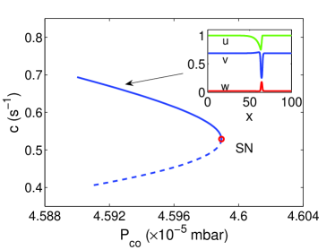
Figure 1: Bifurcation diagram of 1D pulses with respect to the partial pressure of CO. The variable $c$ is the propagating speed of the steady pulse (a representative one is shown in the inset). The turning point (saddle-node bifurcation) is indicated by a red circle. Solid (dashed) lines denote stable (unstable) steady pulse solutions. $T=540K,P_{O_{2}}=1.33\times 10^{-4}mbar$. The inset shows the typical shape of $u$, $v$ and $w$ at the steady state marked by the arrow.

We recall some results for simple, one-dimensional solitary pulses with respect to the variation of $Pco$, as shown in Fig. 1. The travelling speed of a stable solitary pulse decreases as $Pco$ increases. When $Pco$ is above some critical value ($4.599\times 10^{-5}mbar$ in Fig. 1), the medium can not support pulses any more. Checking the leading eigenvalues of the linearization of the system equations we identify the bifurcation at which the pulse is lost as a turning point (or saddle-node) instability: a single eigenvalue crosses zero and becomes positive as the branch of travelling pulses turns around and becomes unstable (saddle-type). In a two-dimensional ring-shaped domain, the shape and stability of travelling pulses is affected by the presence of inert boundaries, as shown in Fig. 2.

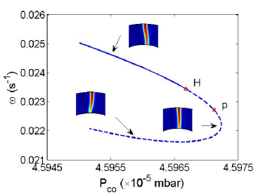
Figure 2: Bifurcation diagram of pulses in a 2D ring showing the influence of the CO partial pressure on the angular speed ($\omega$) of the travelling pulse at stationarity. Point $H$, marked with a red circle, denotes a Hopf bifurcation. Solid (dashed) lines denote stable (unstable) steady pulse solutions. The insets show profiles of O coverage. The color is scaled from blue to red according to the coverage of oxygen from low to high. The leading eigenvalues and corresponding eigenvectors at points $H$ and $p$ are plotted in Fig.  3. The inner and outer dimensionless radius of the ring are 20 and 30 respectively. $T=540K,P_{O_{2}}=1.33\times 10^{-4}mbar;P_{CO}$ is the bifurcation parameter.

The insets show the oxygen coverage profile corresponding to the steady pulse at different locations along the diagram. The inner and outer radius of the ring are fixed at dimensionless values of 20 and 30 respectively (1 unit corresponds to approximately 3.8 ${\mu}m$s). Comparing the bifurcation diagrams in Fig. 2 and 1 shows that the turning point bifurcation is still present, but now we find that the pulse loses stability before the turning point due to a Hopf bifurcation; simulations indicate that this bifurcation is subcritical. We plot the eigenmodes corresponding to the leading eigenvalues at points $H$ and $p$ along the diagram in Fig. 3.

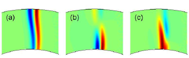
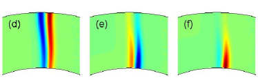
Figure 3: The corresponding eigenmodes of three leading eigenvalues at point $H$ and $p$ as in Fig.  2. (a)-(c) are eigenmodes for point $H$. (a) $\lambda=0.0005$, (b) and (c) $\lambda=-0.0006\pm 0.2591i$. (d)-(f) are eigenmodes for point $p$. (d) $\lambda=0.0026$, (e) $\lambda=0.1172$, (f) $\lambda=0.2324$.

The leading eigenmodes at the Hopf bifurcation point $H$, Fig. 3(b) and 3(c), constitute a complex pair crossing the imaginary axis and rendering the pulse unstable. The spatial structure of these eigenmodes clearly resides close to the inner boundary, suggesting that this boundary is responsible for the instability. An eigenvalue zero corresponding to the rotational invariance is also found; its eigenvector (Fig. 3(a) and 3(d)) can be obtained from the pulse shape by differentiation with respect to $\theta$. When the pulse propagates in the ring, its shape is no longer planar (see the snapshot of a pulse on the stable branch in Fig. 2); it has to curve so as to satisfy the no-flux boundary condition on both curved boundaries. The end of the pulse close to the inner boundary takes a convex shape and it is known that such a convex shape of pulses may lead to instability when the curvature grows above some critical value Mikhailov (1994). We will see this boundary effect on the stability of pulses more clearly below, when we present bifurcation diagrams from a direct continuation in the ring radius. After the Hopf bifurcation, the eigenvalue pair responsible for it collapses on the real axis, giving rise to two real positive eigenvalues close to point $p$. Fig. 3(e) and 3(f) show the corresponding eigenmodes of these two real eigenvalues at point $p$; the absolutely smaller one of the two proceeds to cross zero at the turning point.

For the two-dimensional ring structure, the shape and stability of the pulse solutions are dictated by the choice of $r_{i}$ and $r_{o}$. For more general geometries (e.g. non-concentric boundaries) one can parameterize the geometry through the inner curvature, the outer curvature and the distance between the boundaries. We will look at the effect of geometry taking two distinct one-parameter paths: (a) change radii while keeping the ring width fixed; and (b) fix the outer boundary and vary the inner one.

III.2 Influence of varying the boundary curvature

Figure 4 reflects the influence of the curvature (of both boundaries) on the pulse stability with $r_{o}-r_{i}$ held fixed.

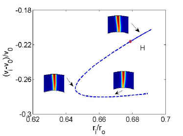
Figure 4: Bifurcation diagram varying the boundary curvatures while fixing ring width. $v_{i}$ is the local velocity of the propagating pulse at the inner boundary. $v_{0}$ is the propagating speed of a one-dimensional pulse. The increase of boundary curvature leads to a pulse instability that is associated with a Hopf bifurcation, followed again by a turning point. $T=540K,P_{O_{2}}=1.33\times 10^{-4}mbar,P_{CO}=4.597\times 10^{-5}mbar$. $r_{o}-r_{i}$ is fixed at 8.

The leading eigenvalues and corresponding eigenmodes at the Hopf bifurcation point are plotted in Fig. 5.

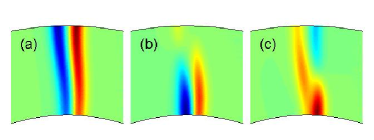
Figure 5: Three leading eigenvalues and corresponding eigenmodes at the Hopf bifurcation point $H$ in Fig. 4. (a) $\lambda=-0.0012$, (b) and (c) $\lambda=-0.0025\pm 0.2899i$.

Similar to the first row of Fig. 3, the eigenmodes corresponding to the eigenvalue pair crossing the imaginary axis show some structure close to the inner boundary, but here both the Hopf and SN bifurcation (at the turning point) are induced by the change of boundary curvature alone. The Hopf bifurcation is again subcritical (as simulations indicate).

In the limit of $r_{i}/r_{o}=1$ as $r_{i}\rightarrow\infty$, we should have an effectively one-dimensional planar pulse with a constant velocity $v_{0}$. As we decrease $r_{i}$, the local curvature of the pulse close to the inner boundary increases and the local shape of the pulse becomes more convex (compare the top inset in Fig. 4 with a planar pulse). This is associated with a decreasing local velocity. For a stable two-dimensional pulse expanding in an infinite medium as a two-dimensional ring (with azimuthally uniform curvature), the propagating velocity (and the pulse stability) increases as the ring grows and the pulse becomes less convex Mikhailov (1994). There also exists a critical curvature above which no pulse solution exists. A pulse “fragment” propagating within a two-dimensional ring structure acquires a non-uniform curvature, so as to satisfy the no-flux boundary conditions applied on both curved boundaries (and the linear speed distribution required for it to propagate coherently). This can lead to a locally concave shape of the pulse (larger local velocity) close to the outer boundary and a locally convex shape (smaller local velocity) close to the inner boundary. The difference in the local curvature of the 2D pulse close to the inert boundaries contributes to the spatial structure of the unstable eigenmodes near the Hopf bifurcation point. We now study how the pulse responds to changes in $r_{i}$ while keeping $r_{o}$ fixed. In this case, as we vary $r_{i}$, both the curvature of the inner boundary and the distance between the two boundaries change. A typical bifurcation diagram with respect to $r_{i}$ with fixed $r_{o}$ is plotted in Fig. 6.

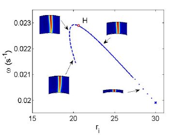
Figure 6: Bifurcation diagram of pulses in a 2D ring showing the influence of varying the inner ring radius $r_{i}$ on the travelling pulse stability. Point $H$, marked with a red circle, denotes a Hopf bifurcation. Solid (dashed) lines denote stable (unstable) steady pulse solutions. For $r_{i}$ close to 30, steady pulse solutions are computed at discrete points. Insets show the profiles of O coverage. The dimensionless outer radius of the ring $r_{o}$ is fixed at 30. $T=540K,P_{O_{2}}=1.33\times 10^{-4}mbar,P_{CO}=4.597\times 10^{-5}mbar$.

When $r_{i}$ approaches the outer ring radius $r_{o}$, the pulse becomes effectively one-dimensional and propagates at a limiting velocity of approximately $0.6s^{-1}$ ($0.02s^{-1}$ for $\omega$ with $r_{o}=30$), consistent with the value read from the one-dimensional pulse bifurcation diagram in Fig. 1. The qualitative structure of the bifurcation diagram in Fig. 6 is similar to that in Fig. 4.

The continuation of pulse solutions with respect to $r_{i}$ for several fixed values of $r_{o}$ is shown in Fig. 7.

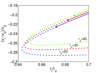
Figure 7: Bifurcation diagram varying the inner ring radius $r_{i}$ while fixing $r_{o}$. $v_{i}$ is the local velocity of the propagating pulse at the inner boundary. $v_{0}$ is the propagating speed of a one-dimensional pulse. The $v_{i}$ associated with the Hopf bifurcation point depends on $r_{o}$.

We see that, at criticality, the pulse speed at the inner boundary (the slowest linear speed along the pulse) does depend on the actual value of $r_{o}$ (and thus the overall pulse shape and its nonuniform curvature). All three stable branches for different $r_{o}$ converge to a distinct point at $r_{i}/r_{o}=1$, that corresponds to the one-dimensional problem (and so do, separately, all three unstable ones).

When the diffusion coefficient is sufficient small, the medium can no longer support a pulse solution; this is associated with a turning point on the continuation curve with respect to the diffusion coefficient at fixed $r_{i}$ and $r_{o}$ (not shown). Scaling both ring radii by a factor of $k$ is equivalent to fixing the geometry but solving a problem with a diffusion coefficient scaled by a factor of $1/k^{2}$. This can be used to rationalize the movement of the bifurcation curves towards the right in Fig. 7: Using increasingly larger $r_{o}$ should lead to a critical $r_{o}$ above which there exists no pulse solution for a given $r_{i}/r_{o}$.

IV Dynamic simulations and experiments

We now consider how the boundary curvature-associated pulse instabilities manifest themselves in time for both simulations and experiments. A dynamic simulation close to (but just beyond) the Hopf bifurcation point shows an initial “tornado like” oscillation of the “tip” of the pulse close to inner boundary. This tip becomes increasingly thinner (as indicated by the color contours) and after some time the pulse “decollates” from the inner boundary and eventually dies (Fig. 8(a)). This transient eventually evolves to the spatially uniform steady state which is stable; thus the simulation is consistent with a subcritical Hopf bifurcation. The limit cycle branch is born unstable and “backwards” in parameter space; the saddle-type limit cycle and its stable manifold constitute the separatrix between the stable pulse and the stable uniform solution when these coexist.

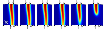
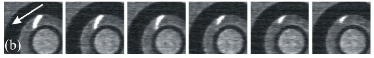
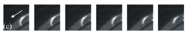
Figure 8: Sequences of snapshots showing the decollation of propagating pulses from the inner boundary of a ring structure. (a) Numerical simulation. The time interval between each snapshot is 2 seconds. Position-fixed arrows are used to show the change of decollating pulse. The arrows are aligned to the boundary of the pulse in the first snapshot. The “tip” of the pulse at the inner boundary first slowly moves toward the left and shrinkes at the same time, then it decollates from the boundary. (b) and (c) are experimental observations. The dark area is TiO₂ and the gray area is Pt(110). The white propagating pulse is a CO-rich one.Experimental conditions: $T=447K,P_{O_{2}}=4\times 10^{-4}mbar$, (b) $P_{co}=3.35\times 10^{-5}mbar$, (c) $P_{co}=2.95\times 10^{-5}mbar$.

Figure 8(b) and 8(c) show this “decollation” mechanism from experimental observations of a CO-rich pulse in a sequence of still shots 0.28 second apart. The direction of motion of the pulse in the ring is denoted by an arrow. The data come from photoemission electron microscopy (PEEM) observations of CO oxidation on micro-designed Pt catalysts; the black areas are 2000 Å tall Ti layers, deposited through microlithography on the Pt(110) single crystal. The inner and outer rings of the ring-shaped Pt “corridor” between the tall Ti “walls” are 12.5 (160) and 20 (180) $\mu$m respectively in Fig. 8(b) (Fig. 8(c)). The experimental conditions are given in the figure caption; one must remember, however, when observing these experiments that diffusion on the Pt(110) crystal is anisotropic. The “thinning” and decollation of the pulse close to the inner boundary can be clearly seen.

V Summary and Conclusions

We studied the effect of operating conditions and of geometry (in particular, of boundary curvature) on the speed and stability of pulses in excitable media; our illustrative model described CO oxidation under high vacuum conditions on Pt(110). The main instability is a decollation that occurs at the inner ring boundary; while the turning point bounding one-dimensional pulses still exists in full two-dimensional studies, the primary destabilization occurs earlier, before the turning point itself. We found that this primary instability involves a (subcritical) Hopf bifurcation, leading to the decollation of the pulse from the inner boundary, and (here) its eventual death.

In microdesigned/microstructured media, pulses often encounter sudden changes in curvature (for example, at corners, or channel exits); a ring geometry -more precisely, families of ring geometries with varying radii- allows for the systematic study of the effect of steady, controlled curvature. This provides insight in the basic “boundary decollation” instability which underpins many of the events occurring in more complex media. Dynamic pattern formation in microchannels is studied in many contexts beyond catalytic reactions (see e.g. recent work in homogeneous reactions Kitahata et al. (2005), and beyond reacting systems in microfluidics Kuksenok et al. (2003); Dreyfus et al. (2003)). Boundary curvature and its variations is, we believe, a crucial factor in all such applications. Additional issues like boundary roughness (statistics of curvature at a much finer scale) as well as the use of active boundaries (e.g. consisting of a different catalyst, see Li et al. (2002)) will modify the results we described here. We believe, however, that the basic reacting front decollation from a curved boundary will be a recurring theme in all these contexts, and an important component of pattern formation in complex heterogeneous media.

Acknowledgements. This work was partially supported by an NSF/ITR grant and by AFOSR (IGK, LQ); LQ gratefully acknowledges the support of a PPPL Fellowship.

References

- Cross and Hohenberg (1993) M. C. Cross and P. C. Hohenberg, Rev. Mod. Phys. 65, 851 (1993).
- Imbihl (2005) R. Imbihl, Catalysis Today 105, 206 (2005).
- Rotermund et al. (1990) H. H. Rotermund, W. Engel, M. Kordesch, and G. Ertl, Nature (London) 343, 355 (1990).
- Jiang et al. (2004) X. Jiang, D. A. Bruzewicz, A. P. Wong, M. Piel, and G. M. Whitesides, Proc. Nat. Acad. Sci. USA 102, 975 (2004).
- Park et al. (1997) M. Park, C. Harrison, P. M. Chaikin, R. A. Register, and D. H. Adamson, Science 276, 1401 (1997).
- Verberg et al. (2004) R. Verberg, C. M. Pooley, J. M. Yeomans, and A. C. Balazs, Phys. Rev. Lett. 93, 184501 (2004).
- Böltau et al. (1998) M. Böltau, S. Walheim, J. Mlynek, G. Krausch, and U. Steiner, Nature (London) 391, 877 (1998).
- Steinbock et al. (1995) O. Steinbock, P. Kettunen, and K. Showalter, Science 269, 1857 (1995).
- Graham et al. (1994) M. D. Graham, I. G. Kevrekidis, K. Asakura, J. Lauterbach, K. Krischer, H. H. Rotermund, and G. Ertl, Science 264, 80 (1994).
- Tusscher and Panfilov (2005) K. H. W. J. T. Tusscher and A. V. Panfilov, Multiscale Model. Simul. 3, 265 (2005).
- Bub et al. (2005) G. Bub, A. Shrier, and L. Glass, Phys. Rev. Lett. 94, 028105 (2005).
- Kaminaga et al. (2005) A. Kaminaga, V. K. Vanag, and I. R. Epstein, Phys. Rev. Lett. 95, 058302 (2005).
- Stone et al. (2004) H. A. Stone, A. D. Stroock, and A. Ajdari, Annu. Rev. Fluid Mech. 36, 381 (2004).
- Joanicot and Ajdari (2005) M. Joanicot and A. Ajdari, Science 309, 887 (2005).
- Stroock et al. (2002) A. D. Stroock, S. K. W. Dertinger, A. Ajdari, I. Mezić, H. A. Stone, and G. M. Whitesides, Science 295, 647 (2002).
- Wolff et al. (2001) J. Wolff, A. G. Papthanasiou, I. G. Kevrekidis, H. H. Rotermund, and G. Ertl, Science 294, 134 (2001).
- Sakurai et al. (2002) T. Sakurai, E. Mihaliuk, F. Chirila, and K. Showalter, Sience 296, 2009 (2002).
- Lucchetta et al. (2005) E. M. Lucchetta, J. H. Lee, L. A. Fu, N. H. Patel, and R. F. Ismagilov, Nature 434, 1134 (2005).
- Agladze et al. (1994) K. Agladze, J. P. Keener, S. C. Muller, and A. Panfilov, Science 264, 1746 (1994).
- Hartmann et al. (1996) N. Hartmann, M. Bär, I. G. Kevrekidis, K. Krischer, and R. Imbihl, Phys. Rev. Lett. 76, 1384 (1996).
- Bär et al. (1996) M. Bär, A. K. Bangia, I. G. Kevrekidis, G. Haas, H. H. Rotermund, and G. Ertl, J. Phys. Chem. 100, 19106 (1996).
- Tyson and Keener (1988) J. J. Tyson and J. P. Keener, Physica D 32, 327 (1988).
- Mikhailov (1994) A. S. Mikhailov, Foundations of Synergetics I: Distributed Active systems (Springer, New York, 1994).
- Krishnan et al. (1999) J. Krishnan, I. G. Kevrekidis, M. Or-Guil, M. G. Zimmerman, and M. Bär, Comput. Methods Appl. Mech. Engrg. 170, 253 (1999).
- Or-Guil et al. (2001) M. Or-Guil, J. Krishnan, I. G. Kevrekidis, and M. Bär, Phys. Rev. E 64, 046212 (2001).
- Krishnan et al. (2001) J. Krishnan, K. Engelborghs, M. Bär, K. Lust, D. Roose, and I. G. Kevrekidis, Physica D 154, 85 (2001).
- Bär et al. (1994) M. Bär, N. Gottschalk, M. Eiswirth, and G. Ertl, J. Chem. Phys. 100, 1202 (1994).
- Krischer et al. (1992) K. Krischer, M. Eiswirth, and G. Ertl, J. Chem. Phys. 96, 9161 (1992).
- Kelley (1995) C. T. Kelley, Iterative Methods for Linear and Nonlinear Equations, vol. 16 of Frontiers in Applied Mathematics (SIAM, Philadelphia, 1995).
- Rowley and Marsden (2000) C. W. Rowley and J. E. Marsden, Physica D 142, 1 (2000).
- Rowley et al. (2003) C. W. Rowley, I. G. Kevrekidis, J. E. Marsden, and K. Lust, Nonlinearity 16, 1257 (2003).
- Beyn and Thümmler (2004) W. J. Beyn and V. Thümmler, SIAM J. Appl. Dyn. Syst. 3, 85 (2004).
- Kitahata et al. (2005) H. Kitahata, A. Yamada, S. Nakata, and T. Ichino, J. Phys. Chem. A 109, 4973 (2005).
- Kuksenok et al. (2003) O. Kuksenok, D. Jasnow, J. Yeomans, and A. C. Balazs, Phys. Rev. Lett. 91, 108303 (2003).
- Dreyfus et al. (2003) R. Dreyfus, P. Tabeling, and H. Willaime, Phys. Rev. Lett. 90, 144505 (2003).
- Li et al. (2002) X. Li, I. G. Kevrekidis, M. Pollmann, A. G. Papathanasiou, and H. H. Rotermund, Chaos 12, 190 (2002).