Multidimensional semi-gap solitons in a periodic potential

Abstract

The existence, stability and other dynamical properties of a new type of multi-dimensional (2D or 3D) solitons supported by a transverse low-dimensional (1D or 2D, respectively) periodic potential in the nonlinear Schrödinger equation with the self-defocusing cubic nonlinearity are studied. The equation describes propagation of light in a medium with normal group-velocity dispersion (GVD). Strictly speaking, solitons cannot exist in the model, as its spectrum does not support a true bandgap. Nevertheless, the variational approximation (VA) and numerical computations reveal stable solutions that seem as completely localized ones, an explanation to which is given. The solutions are of the gap-soliton type in the transverse direction(s), in which the periodic potential acts in combination with the diffraction and self-defocusing nonlinearity. Simultaneously, in the longitudinal (temporal) direction these are ordinary solitons, supported by the balance of the normal GVD and defocusing nonlinearity. Stability of the solitons is predicted by the VA, and corroborated by direct simulations.

I Introduction

Recently, a variety of two- and three-dimensional (2D and 3D) solitons have been investigated in models based on the nonlinear Schrödinger (NLS) or Gross-Pitaevskii (GP) equations with a spatially periodic potential and cubic nonlinearity, see a review review . The physical models of this type emerge in the context of Bose-Einstein condensation (BEC) multi-d ; bmsEPL ; Yang ; Estoril ; bms ; mih , where the periodic potential is created as an optical lattice (OL), i.e., interference pattern formed by coherent beams illuminating the condensate, and in nonlinear optics, where similar models apply to photonic crystals PhotCryst . A different but allied setting is provided by a cylindrical OL (“Bessel lattice”), which can also support stable 2D Kartashov and 3D mihalache solitons. Additionally, models combining a periodic lattice potential and saturable nonlinearity give rise to 2D solitons, that were predicted in Ref. PhotorefrPrediction and observed in several experiments in photorefractive media, including fundamental solitons Photorefr2Dsolitons and vortices PhotorefrVortices . It is also relevant to mention that experimental observation of spatiotemporal self-focusing of light in silica waveguide arrays, in the region of anomalous group-velocity dispersion (GVD), was reported in Ref. Cheskis .

In models with the cubic nonlinearity, these solutions were investigated in a quasi-analytical form, which combines the variational approximation (VA) va to predict the shape of the solitons, and the Vakhitov-Kolokolov (VK) criterion vk to examine their stability. Final results were provided by numerical methods, relying upon direct simulations of the underlying NLS/GP equations. A conclusion obtained by means of these methods is that, unlike their 1D counterparts, multi-dimensional solitons in periodic potentials can exist only in a limited domain of the $\left(N,\varepsilon\right)$ plane, where $N$ and $\varepsilon$ are the norm of the solution and strength of the OL potential, respectively. The most essential limitation on the existence domain of 2D solitons is that $N$ cannot be too small (in a general form, a minimum value of the norm, as a necessary condition for the existence of 2D solitons supported by lattice potentials, was discussed in Ref. efremidis ). Unlike it, $\varepsilon$ may be arbitrarily small, as even at $\varepsilon=0$ the 2D NLS equation has a commonly known weakly unstable solution in the form of the Townes soliton, at a single value of the norm, $N=N_{\mathrm{T}}$ Townes ($N_{\mathrm{T}}\approx 11.7$ for the NLS equation in the usual 2D form, $iu_{t}+\nabla^{2}u+|u|^{2}u=0$). Small finite $\varepsilon$ gives rise to a narrow stability region,

$$0<N_{\mathrm{T}}-N<\left(\Delta N\right)_{\max}\sim\varepsilon$$ (1)

for the 2D solitons bmsEPL . Crossing the lower border of the existence domain (1) leads to disintegration of the localized state into linear Bloch waves (radiation) bs .

In the case of the attractive cubic nonlinearity (which corresponds to BEC where atomic collisions are characterized by a negative scattering length, while this is the case of the normal, self-focusing Kerr effect), 2D and 3D solitons can be stabilized not only by the potential lattice whose dimension is equal to that of the ambient space, but also by low-dimensional periodic potentials, whose dimension is smaller by one, i.e., 2D and 3D solitons can be stabilized by a quasi-1D Estoril ; bms or quasi-2D Estoril ; bms ; mih OL, respectively [in the former case, the qualitative estimate (1) for the width of the stability region at small $\varepsilon$ is correct too]; however, 3D solitons cannot be stabilized by a quasi-1D lattice potential Estoril ; bms [this is possible if the 1D potential is applied in combination with the Feshbach-resonance management, i.e., periodic reversal of the sign of the nonlinearity coefficient Warsaw , or in combination with dispersion management, i.e., periodically alternating sign of the local GVD coefficient Michal ]. Solitons can exist in such settings because the attractive nonlinearity provides for stable self-localization of the wave function in the free direction (one in which the low-dimensional potential does not act), essentially the same way as in the 1D NLS equation, and, simultaneously, the lattice stabilizes the soliton in the other directions (in the 3D model with the quasi-1D OL potential, the self-localization in the transverse 2D subspace, where the potential does not act, is possible too, but the resulting soliton is unstable, the same way as the above-mentioned Townes soliton). An important aspect of settings based on the low-dimensional OL potentials is mobility of the solitons along the free direction, which opens the way to study collisions between solitons and related dynamical effects bms .

In the case of defocusing nonlinearity, which corresponds to a positive scattering length in the BEC, or self-defocusing nonlinearity in optics (negative Kerr effect), the soliton cannot support itself in the free direction. Localization in that direction may be provided by an additional external confining potential; however, the resulting pulse is not a true multidimensional soliton, but rather a combination of a gap soliton (a weakly localized state created by the interplay of the repulsive nonlinearity and periodic potential multi-d ),which was recently created experimentally in a 1D BEC Oberthaler ) in the direction(s) affected by the OL, and of a Thomas-Fermi state, directly confined by the external potential in the remaining direction bms .

Thus, no soliton can be supported by a low-dimensional lattice in the BEC model (GP equation) with self-repulsion (the latter corresponds to the most common situation in the experiment Oberthaler ). On the other hand, a new possibility may be considered in terms of nonlinear optics. Indeed, one may combine three physically relevant ingredients, viz., (i) an effective periodic potential in the transverse direction(s), while the medium is uniform in the propagation direction, (ii) self-defocusing nonlinearity, and (iii) normal GVD. The latter is readily available, as most optical materials feature normal GVD, in compliance with its name. As concerns the negative cubic nonlinearity, it is possible in semiconductor waveguides, or may be engineered artificially, through the cascading mechanism, in a quadratically nonlinear medium with a proper longitudinal quasi-phase-matching QPM . Also quite encouraging for the study of multidimensional solitons proposed in this work are recent observations of 1D jason1 and 2D Photorefr2Dsolitons solitons in optically induced waveguide arrays (photonic lattices) with self-defocusing nonlinearity.

The setting outlined above can be realized in both 2D and 3D geometry, where the necessary transverse modulation of the refractive index is provided, respectively, by the transverse structure in a planar photonic-crystal waveguide, or in a photonic-crystal fiber. To the best of our knowledge, in either case the model is a novel one. A soliton in this medium, if it exists, will be of a mixed type: in the transverse direction(s), it is, essentially, a 1D or 2D spatial gap soliton, supported by the combination of the effective periodic potential and self-defocusing nonlinearity, while in the longitudinal direction it is a temporal soliton of the ordinary type, which is easily sustained by the joint action of the self-defocusing nonlinearity and normal GVD. Thus, one may anticipate stable spatiotemporal solitons, alias “light bullets”, in this model. Due to their mixed character, they may be called semi-gap solitons. The issue is of considerable interest in view of the lack of success in experiments aimed at the creation of “bullets” in more traditional nonlinear-optical settings review . The only earlier proposed scheme for the stabilization of 2D spatiotemporal optical solitons in periodic structures, that we are aware of, assumed the use of a planar waveguide with constant self-focusing nonlinearity and longitudinal dispersion management WarsawDM .

On the other hand, it is necessary to stress that, rigorously speaking, completely localized solutions cannot exist in the present model: its linear spectrum cannot give rise to any true bandgap, in which genuine solitons could be found (see below); instead, one may expect the existence of quasi-solitons, consisting of a well-localized “body” and small nonvanishing “tails” attached to it. Nevertheless, we will produce families of solutions which seem as stable perfectly localized objects. This is possible because the “tails” may readily turn out to be so tiny that they remain completely invisible in numerical results (possibly being smaller than the error of the numerical scheme), and, of course, they will be invisible in any real experiment. An explanation to this feature is provided by the fact that bandgaps, which “almost exist” in the system’s spectrum, do not exist in the strict sense because they are covered by linear modes with very large wavenumbers. As shown in Ref. Isaac , in this case the amplitude of the above-mentioned tails (which are composed of the linear modes with very large wavenumbers) is exponentially small. In fact, families of stable “practically existing” solitons in a second-harmonic-generating system with opposite signs of the GVD at the fundamental-frequency and second harmonics, where solitons cannot exist in the rigorous mathematical sense, were explicitly found in that system, in both multi- Isaac and one- Kale dimensional settings. Implicitly (without discussion of this issue), “practically existing” solitons (although, in this case, they were unstable against small perturbations) were also found in a recent work Alejandro , which was dealing with a 2D model of a planar nonlinear waveguide with the cubic nonlinearity, that features a Bragg grating in the longitudinal direction, and is uniform along the transverse coordinate. In the latter model, true solitons cannot exist, as the spectrum of the system does not support a full bandgap.

The objective of the present paper is to explore 2D and 3D spatiotemporal solitons (which may be, strictly speaking, “quasi-solitons”, in the above sense, but feature completely localized shapes) and their stability in the proposed medium. In Section 2 we fix the mathematical form of the 2D version of the model, analyze its spectrum, and apply the VA to the study of solitons. In Section 3, direct numerical results demonstrating the existence of very robust 2D solitons, and their delocalization when the lattice strength $\varepsilon$ becomes too small, are reported (the comparison with the VA prediction shows that the VA provides for a crude approximation in the present model). In Section 4, we additionally consider the effect of variation of the nonlinearity coefficient along the propagation distance on 2D solitons. Finally, numerical results for 3D solitons are collected in Section 5, and the paper is concluded by Section 6.

II Formulation and variational analysis of the two-dimensional model

The model of a planar waveguide corresponding to the outline given above is based on the following variant of the 2D NLS equation for the local amplitude $u(z,x,t)$ of the electromagnetic field:

$$iu_{z}-\frac{1}{2}u_{tt}+\frac{1}{2}u_{xx}+\varepsilon\cos(2x)u-|u|^{2}u=0,$$ (2)

where $z$ is the propagation distance, $x$ is the transverse coordinate, and $t$ is the reduced time, defined the same way as in fiber optics. The signs in front of the GVD ($u_{tt}$) and cubic terms correspond, as said above, to the normal GVD and self-defocusing nonlinearity, $\varepsilon$ is the amplitude of the transverse modulation of the refractive index (which is assumed sinusoidal, but the results will be nearly the same for more realistic forms of the modulation which correspond to the actual photonic-crystal structure), and the period of the modulation is scaled to be $\pi$. Dynamical invariants of Eq. (2) are the norm of the solution (in optics, it is the total energy),

$$N\equiv\int_{-\infty}^{+\infty}dx\int_{-\infty}^{+\infty}dt|u(z,x,t)|^{2},$$ (3)

together with the longitudinal momentum and Hamiltonian,

$$P = i\int_{-\infty}^{+\infty}dx\int_{-\infty}^{+\infty}dt~{}u_{t}^{\ast}u,$$ (4)

$$H = \int_{-\infty}^{+\infty}dx\int_{-\infty}^{+\infty}dt\left[\frac{1}{2}\left|u_{x}\right|^{2}-\frac{1}{2}\left|u_{t}\right|^{2}+\right.$$ (5)

$$\left.\frac{1}{2}|u|^{4}-\varepsilon\cos(2x)|u|^{2}\right].$$

To find the linear spectrum of the model, one looks for solutions to the linearized version of Eq. (2) as

$$u(z,t,x)=\exp\left(ikz-i\omega t\right)F_{E}(x),$$ (6)

where $k$ is a real propagation constant, $\omega$ is an arbitrary real eigenvalue,

$$E\equiv\omega^{2}-2k,$$ (7)

and $F_{E}(x)$ is a solution of the Mathieu equation,

$$F^{\prime\prime}+2\varepsilon\cos\left(2x\right)F+EF=0,$$ (8)

corresponding to the eigenvalue $E$. It is commonly known that the Mathieu equation gives rise to bandgaps in its own spectrum, i.e., to forbidden intervals of the values of $E$, within which no regular quasi-periodic solutions of Eq. (8) can be found. However, since all large values of $E$ ($E\gg\varepsilon$) belong to the allowed band, where such solutions exist, it is obvious that no value of $k$ may fall in a forbidden bandgap. Indeed, using Eq. (7), one can construct any real value of the propagation constant as $k=\left(\omega^{2}-E\right)/2$, taking very large $E$ and, accordingly, very large $\omega$.

On the other hand, the same consideration suggests that, in some cases, the necessary values of $E$ and $\omega$ may be very large indeed. It was shown, in a general form, in Ref. Isaac that short-period waves corresponding to such large parameters, which build up into a possible “tail” attached to the soliton’s “body” (that makes it a quasi-soliton), will have an exponentially small amplitude, rendering the tail totally negligible (in particular, it may be completely invisible in numerical solutions). Therefore, it makes sense to look for “practically existing” solitons in the present model.

We start searching for stationary solutions of the “mixed” type, which, as explained above, are expected to feature a gap-soliton (weakly localized) shape along $x$ and strong ordinary localization in $t$, by adopting the following variational ansatz,

$$u(z,x,t)=Ae^{ikz}\left[x^{-1}\sin(ax)\right]\mathrm{sech}(\alpha t),$$ (9)

where $a$ and $\alpha$ are, respectively, the transverse and longitudinal inverse widths of the soliton, and $A$ is its amplitude. Using the obvious Lagrangian representation of Eq. (2) and well-known VA formalism va , one can readily derive the following equations for the parameters of the ansatz,

$$a=\left(\frac{3\varepsilon}{1+(N/3\pi)^{2}}\right)^{1/3},$$ (10)

$$\alpha=\frac{aN}{3\pi},~{}A=\frac{N}{\sqrt{6}\pi},~{}k=\varepsilon-\frac{\varepsilon^{2/3}}{2\left(27\pi^{2}\right)^{1/3}}\frac{27\pi^{2}+5N^{2}}{\left(9\pi^{2}+5N^{2}\right)^{2/3}},$$ (11)

where $N$ is the norm defined by Eq. (3). It follows from these equations that the condition $dk/dN<0$, i.e., the necessary stability condition, according to the above - mentioned VK criterion vk , always holds, as shown in Fig. 1.

Figure 1: The propagation constant vs. norm for the 2D solitons, as predicted by the variational approximation, Eq. (11), for different values of the strength of the periodic potential $\varepsilon$. The negative slope, $dk/dN<0$, implies stability of the solitons according to the Vakhitov-Kolokolov criterion.

The stability of the soliton families, predicted by the VK criterion as per Fig. 1, is, generally, corroborated by direct numerical simulations, see the next section (with a caveat that the VA predicts the shape of the solitons in only a qualitatively correct form, as explained below). However, it should also be mentioned that the applicability of the VK criterion to gap solitons in lattice models has never been proven, therefore one should apply this method with due care. In particular, it is known that the gap solitons may be unstable in some cases when they are expected to be VK-stable VK- , which is not very surprising, as the VK criterion ignores complex stability eigenvalues, that may give rise to oscillatory instabilities. More perplexing is the fact that some gap-soliton families in a lattice model with the cubic-quintic nonlinearity, that are formally predicted to be VK-unstable, are in reality completely stable VK+ .

To complete the discussion of the VA, it is necessary to notice that ansatz (9) is irrelevant if it predicts $a\ll 1$, as it would mean that the soliton is very broad in the $x$-direction, and it does not feel the underlying lattice structure, $\cos(2x)$ in Eq. (2). We therefore limit the applicability of the VA by a (roughly defined) condition, $a>1$. According to Eq. (10), this implies that the potential must be strong enough,

$$\varepsilon>\frac{1}{3}\left(1+\frac{N^{2}}{9\pi^{2}}\right).$$ (12)

III Numerical results for two-dimensional solitons

Direct simulations of Eq. (2) (propagation in $z$) started with an initial localized waveform, which we took as ansatz (9) with the parameters predicted by Eqs. (11), or just a Gaussian with rather arbitrary parameters – for instance,

$$u(x,t,0)=A\exp[-\frac{a}{2}(x^{2}+t^{2})].$$ (13)

It was observed that the initial waveform undergoes intense evolution, shedding off some radiation waves that were absorbed at edges of the integration domain. The domain was large enough – in most cases, $\left(-8\pi,+8\pi\right)$ in both directions ($x$ and $t$) – so that the solitons, which are typically well localized within a region $\left(-5,+5\right)$, see Figs. 2, 3, 7, and 9 below, are not affected by the absorbers.

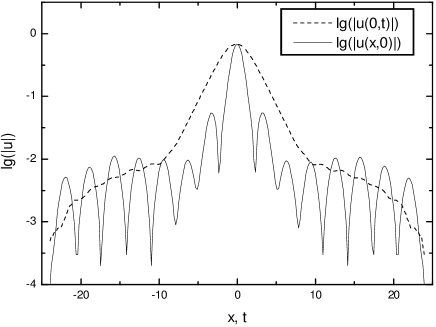
Figure 2: Cross sections of a typical established 2D soliton of the semi-gap type. It has self-trapped from the initial configuration (13) with $A=1$ and $a=1$. The solid and dashed lines represent, respectively, the sections along the transverse directions $x$ at $t=0$, and temporal direction $t$ at $x=0$. The shapes of the cross sections are displayed on the logarithmic scale, to illustrate the fundamental observation of the practical vanishing of the tails attached to the soliton’s “body”.

The evolution of the pulse ends with the establishment of a 2D stationary soliton, without any visible tails, as shown on the logarithmic scale in Fig. 2. It is relevant to mention that, as seen from Figs. 2 and 3, the characteristic sizes of the soliton in the $x$ and $t$ directions are on the same order of magnitude, hence the values of the GVD coefficient and its effective lattice-diffraction counterpart are, roughly, equal.

In fact, the solitons self-trap even from the initial configurations that are quite different from their final shape, which attests to strong robustness of the solitons. The soliton’s stability was then additionally tested against small random perturbations, by simulating the evolution of the initial configuration $U(x,t)=U_{0}(x,t)[1+\sigma u_{p}(x,t)]$, where $U_{0}(x,t)$ is the numerically found soliton, $\sigma$ is a small amplitude of the perturbation, and $u_{p}(x,t)$ is a random function. An example of a stable localized state self-trapped from the initial Gaussian (13) with $A=1$ and $a=1$, with the norm $N_{0}=\pi$, is displayed in Fig. 3.

It should be said that direct comparison of the VA predictions with the numerical results shows only a qualitative agreement: for example, the VA predicts, with the same value of the norm, a soliton whose width in the temporal direction exceeds the actual width of the soliton in Fig. 3, by  factor in excess of $2$, and, accordingly, the amplitude of the numerically found soliton significantly exceeds that predicted by the VA. Therefore, the VA provides for only a crude approximation in this model; nevertheless, its qualitative predictions, such as the stability of the solitons predicted by the VK criterion, are correct. In this connection, it is relevant to mention that no good version of VA has been thus far proposed for gap solitons (this technical issue was considered, in some detail, in Ref. Arik ), and the solitons in the present model are still more complex objects.

.

Figure 3: A stable localized solution of Eq. (2) with $\varepsilon=2.0$, produced from the initial Gaussian pulse (13) with the initial norm $N_{0}=\pi$. The amplitude, inverse width along the temporal direction, and norm of this localized state are $A=0.74$, $\alpha=0.56$, and $N=2.29$, respectively. Note that $27\%$ of the initial norm was lost with emitted radiation in the course of the evolution. Notice that the soliton features no extended tail.

Further numerical analysis of the 2D model has demonstrated that, following the known pattern of the delocalization transition of 2D solitons in lattice potentials bs , the soliton solutions cease to exist when the strength of the periodic potential $\varepsilon$ or the norm of the localized state $N$ fall below some critical values. In this case, the localized waveform undergoes disintegration, transforming into a quasi-linear nonstationary extended state. This state keeps expanding until it eventually hits edge absorbers, thus completely disappearing. Naturally, the expansion occurs faster in the temporal (alias longitudinal) direction, where it is not impeded by any potential structure. Figure 4 illustrates the disintegration of the localized state (the one from Figure 3), following gradual decrease of $\varepsilon$ along the propagation direction. It is relevant to stress that the disintegration of the soliton at small $\varepsilon$ is inevitable, as Eq. (2) with $\varepsilon=0$ has no 2D soliton solution, unlike the Townes soliton, which would be a solution for the equation with $\varepsilon=0$ and reverse sign in front of the $u_{xx}$ term.

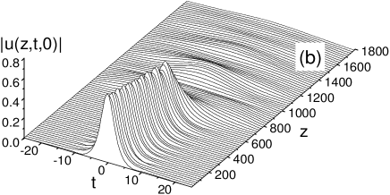
Figure 4: Dynamical disintegration of the localized state shown in Fig. 3 as a result of a gradual decrease of the strength of the periodic potential along the propagation distance, so as $\varepsilon(z)=\varepsilon_{0}(1-z/z_{\mathrm{end}})$, with $\varepsilon_{0}=2$ and $z_{\mathrm{end}}=1800$. Cross sections of the wave profile are displayed: (a) along the transverse coordinate $x$; (b) in the temporal direction $t$. The delocalization occurs around $z=650$, at $\varepsilon$ close to a critical value, $\varepsilon_{\mathrm{cr}}\simeq 1.3$.

Detecting the delocalization transition of the semi-gap solitons at critical values of the nonlinear coefficient (or rescaled norm) and/or the strength of the periodic potential can be used to locate the lower border of their existence region in the parameter space $\left(N,\varepsilon\right)$. Actually, the transition from the localized state to the extended one is quite steep (see Fig. 5), which allows quite accurate determination of the critical values of the parameters. However, delineating the full existence region of the semi-gap solitons is a harder problem, as the limiting effect at large values of the norm, which determines the upper border, is splitting of the soliton (see below), rather than collapse (singularity formation) in the case of lattice gap solitons with the self-focusing nonlinearity bmsEPL . Precise shapes of the existence and stability domains of lattice gap solitons can be rather complex, as shown in Ref. Kartashov for the case of saturable nonlinearity.

Accurate determination of the full stability borders for the solitons in the present model, going beyond the use of the VK criterion and collection of typical examples of direct simulations, will be a subject of separate work.

Figure 5: The amplitude of the 2D semi-gap soliton abruptly decays at the point of the delocalization transition, which was displayed in Fig. 4. The present figure illustrates the steepness of the transition at $\varepsilon\simeq 1.3$, with the slowly decreasing strength of the periodic potential, starting from $\varepsilon=2.0$.

Finally, Eq. (2) features obvious Galilean invariance in the longitudinal ($t$) direction, which makes it possible to generate a boosted soliton $u_{c}$, with an arbitrary inverse-velocity shift $c$, from a given soliton $u$, as

$$u_{c}(z,t)=u(z,t-cz)e^{-i\left(c^{2}/2\right)z-ict}.$$

The use of such two pulses with the $c_{1}\neq c_{2}$ makes it possible to study collisions between the moving solitons, which, however, should be a subject of a separate work.

IV Effects of nonlinearity modulation

As the nonlinearity is a key factor necessary for the existence of solitons, in this section we address response of the 2D solitons to variation of the nonlinearity strength along the propagation coordinate, $z$. In nonlinear optics, a variable nonlinearity coefficient can be created by dint of different physical mechanisms, such as variation of a dopant concentration, optically controlled photorefraction, or simply by using a variable thickness of the planar waveguide.

Thus, we replace Eq. (2) by its variant which includes a variable nonlinear coefficient $\chi(z)$,

$$iu_{z}-\frac{1}{2}u_{tt}+\frac{1}{2}u_{xx}+\varepsilon\cos(2x)u-\chi(z)|u|^{2}u=0.$$ (14)

Then, we follow the transformation of the soliton with slow increase or decrease of $\chi(z)$. Figure 6 displays the evolution of the soliton’s parameters as the nonlinearity coefficient gradually increases ten-fold.

Figure 6: The evolution of the norm ($N$), amplitude ($A$), and inverse temporal width ($\alpha$) resulting from the slow linear increase of the nonlinear coefficient $\chi$ in Eq. (2), $\chi(z)=1+\gamma z/z_{\mathrm{end}}$, with $\gamma=9$ and $0<z<z_{\mathrm{end}}=2000$. Note significant decrease of the norm $N$, opposed by little variation of $A$ and $\alpha$. The initial localized state is the same as in Fig. 3.

In this case, Fig. 7 shows that the final waveform, corresponding to $\chi=10$, has not changed notably compared to initial one (see Fig. 3), which implies that the increase of the nonlinearity is countered by the loss of the norm. The excess norm is shed off with linear waves which are absorbed on the domain boundaries. It appears that the shape of the localized wave, being weakly sensitive to the value of the norm (hence, to the strength of the nonlinearity too), is actually fixed by the strength $\varepsilon$ of the periodic potential. This shape-invariance property of the mixed-type solitons is very different from what is manifested by both ordinary solitons and gap solitons per se, whose shapes are particularly sensitive to the strength of the nonlinearity, at a fixed amplitude of the periodic potential.

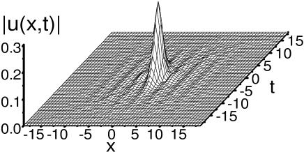
Figure 7: The final shape of the soliton from Fig. 3, established after by slow increase of the nonlinearity by a factor of $10$, as illustrated in the previous figure. Note that an extended tail attached to the soliton does not appear in this case either.

If the coefficient of nonlinearity slowly decreases, as $\chi(z)=1-z/z_{\mathrm{end}}$ with $z_{\mathrm{end}}=2000$, the disintegration of the localized state is observed when falls to the level of $\chi\simeq 0.5$, resembling the picture in Fig. 4. Thus, we conclude that the strengths of both the periodic potential and nonlinearity must exceed some critical values in order to sustain the localized states. In this respect, the multidimensional semi-gap solitons resemble regular gap solitons in lattice potentials efremidis ; bs .

One of characteristic features of ordinary solitons in 1D nonintegrable systems is splitting of the soliton when the GVD coefficient grimshaw or nonlinearity Radik is abruptly changed. In the present model, one can observe a similar effect for 2D solitons. Figure 8 displays an example of the splitting of a soliton into two fragments, which then separate along the free direction $t$, after the nonlinearity coefficient was suddenly increased by an order of magnitude.

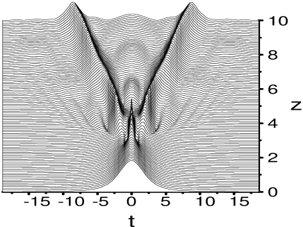
Figure 8: Splitting of the soliton from Fig. 2 along the free direction $t$, following the rapid increase of the nonlinear coefficient by a factor of $10$, which is performed by setting $\chi(z)=1+\gamma\tanh(4z/z_{\mathrm{end}})$ in Eq. (14), with $\gamma=9$ and $z_{\mathrm{end}}=10$.

V The three-dimensional case

The 3D version of Eq. (2) has a straightforward form,

$$iu_{z}-\frac{1}{2}u_{tt}+\frac{1}{2}(u_{xx}+u_{yy})+\varepsilon[\cos(2x)+\cos(2y)]u-|u|^{2}u=0.$$ (15)

Similarly to the 2D case, stationary solutions to Eq. (15) can be numerically found by using a Gaussian pulse as the initial condition and propagating in $z$. Stability of the 3D solitons was verified by simulating the evolution of a soliton with a random perturbation added to it. As well as in the 2D case, the simulations were performed with the absorbers placed at borders of the integration domain (under the condition that the length of the domain was much larger than a characteristic size of the soliton). As a result, it was concluded that robust 3D solitons exist as generic solutions, without any visible tails attached to them. An example of a stationary 3D soliton, which was found to be quite robust in stability simulations, is displayed in Fig. 9. In particular, Fig. 9(b) clearly demonstrates that, as well as in the 2D case, the soliton has, roughly, equal sizes in the spatial and temporal directions, i.e., the GVD and diffraction modified by the periodic potential play equally important roles in supporting the solitons.

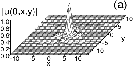
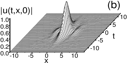
Figure 9: A three-dimensional stationary soliton solution to Eq. (15) with $\varepsilon=2.0$ is shown through its two cross sections: (a) perpendicular to the free direction, in the $t=0$ plane, and (b) parallel to the free direction, in the $y=0$ plane. The soliton was obtained by direct propagation in $z$ of an initial Gaussian with the norm $N_{0}=2\pi$. The norm of the established soliton is $N=4.16$, i.e., a third of the initial norm was lost in the course of the adjustment of the initial pulse to the stationary shape of the 3D soliton.

Besides the fundamental 3D pulses, such as the one displayed in Fig. 9, the model can also support 3D solitons with embedded vorticity. Analogy with known results for gap-soliton vortices in the 2D lattice models GapVortex suggests that the vortex solitons too may easily be stable in the present model. However, detailed investigation of the vortex solutions, as well as collecting systematic data about the family of the fundamental 3D solitons, requires numerous runs of lengthy simulations of the 3D equation, which is beyond the scope of the present paper.

VI Conclusion

In this work, we have proposed a new type of the multidimensional model in nonlinear optics. It combines self-defocusing nonlinearity and normal group-velocity dispersion with periodic modulation of the local refractive index in the one or two transverse directions (in the 2D and 3D models, respectively). Strictly speaking, multidimensional (spatiotemporal) solitons cannot exist in media of this type, as the system’s spectrum contains no true bandgap. Nevertheless, solitons which seem as completely localized ones are predicted by the variational approximation, and found in direct simulations. These solitons are solutions of a mixed type, as in the free (longitudinal, alias temporal) direction they are regular solitons, while in the transverse direction(s) they are objects of the gap-soliton type (hence the solution as a whole was called a semi-gap soliton). The existence of the solitons requires that both the norm of the solution (in other words, the nonlinearity strength $\chi$) and the strength $\varepsilon$ of the spatially periodic transverse potential exceed certain minimum values, otherwise the pulses decay into linear waves. Actually, the solitons are much more sensitive to $\varepsilon$ than to $\chi$.

The results reported in this paper call for further work, that should be aimed at accurate identification of borders of the solitons’ stability regions, especially in the 3D model (which requires running very massive simulations), investigation of collisions between solitons, that may move freely in the longitudinal direction, and the study of vortex solitons in the 3D case.

References

- (1) B. A. Malomed, D. Mihalache, F. Wise, and L. Torner, J. Opt. B: Quant. Semicl. Opt. 7, R53 (2005).
- (2) B. B. Baizakov, V. V. Konotop, M. Salerno, J. Phys. B 35, 5105 (2002); E. A. Ostrovskaya and Y. S. Kivshar, Phys. Rev. Lett. 90, 160407 (2003); H. Sakaguchi and B. A. Malomed, J. Phys. B 37, 1443 (2004).
- (3) B. B. Baizakov, B. A. Malomed and M. Salerno, Europhys. Lett. 63, 642 (2003).
- (4) J. Yang and Z. Musslimani, Opt. Lett. 23, 2094 (2003); Y. V. Kartashov, A. A. Egorov, L. Torner, D. N. Christodoulides, Opt. Lett. 29, 1918 (2004).
-
(5)
B. B. Baizakov, M. Salerno, and B. A. Malomed, in
Nonlinear Waves: Classical and Quantum Aspects, (Kluwer Academic
Publishers, Dordrecht, 2004) edited by F. Kh. Abdullaev and V. V. Konotop,
p. 61; also available at
http://rsphy2.anu.edu.au/~asd124/Baizakov_2004_61_Nonlinear Waves.pdf - (6) B. B. Baizakov, B. A. Malomed and M. Salerno, Phys. Rev. A 70, 053613 (2004).
- (7) D. Mihalache, D. Mazilu, F. Lederer, Y. V. Kartashov, L.-C. Crasovan, and L. Torner, Phys. Rev. E 70, 055603 (2004).
- (8) P. Xie, Z.-Q. Zhang, and X. Zhang, Phys. Rev. E 67, 026607 (2003); A. Ferrando, M. Zacarés, P. Fernández de Córdoba, D. Binosi, and J. A. Monsoriu, Opt. Exp. 11, 452 (2003); ibid. 12, 817 (2004).
- (9) Y. V. Kartashov, V. A. Vysloukh, and L. Torner, Phys. Rev. Lett. 93, 093904 (2004); 94, 043902 (2005).
- (10) D. Mihalache, D. Mazilu, F. Lederer, B. A. Malomed, Y. V. Kartashov, L.-C. Crasovan, and L. Torner, Phys. Rev. Lett. 95, 023902 (2005).
- (11) N. K. Efremidis, S. Sears, D. N. Christodoulides, J. W. Fleischer, and M. Segev, Phys. Rev. E 66, 046602 (2002).
- (12) J. W. Fleischer, M. Segev, N. K. Efremidis, and D. N. Christodoulides, Nature 422, 147 (2003).
- (13) D. N. Neshev, T. J. Alexander, E. A. Ostrovskaya, and Y. S. Kivshar, H. Martin, I. Makasyuk, and Z. Chen, Phys. Rev. Lett. 92, 123903 (2004); J. W. Fleischer, G. Bartal, O. Cohen, O. Manela, M. Segev, J. Hudock, and D. N. Christodoulides, ibid. 92, 123904 (2004); G. Bartal, O. Manela, O. Cohen, J. W. Fleischer, and M. Segev, ibid. 95, 053904 (2005).
- (14) D. Cheskis, S. Bar-Ad, R. Morandotti, J. S. Aitchison, H. S. Eisenberg, Y. Silberberg, and D. Ross, Phys. Rev. Lett. 91, 223901 (2003).
- (15) D. Anderson, Phys. Rev. A27, 1393 (1983); B. A. Malomed, Progr. Optics 43, 69 (2002).
- (16) M. G. Vakhitov and A. A. Kolokolov, Radiophys. Quantum Electron. 16, 783 (1973).
- (17) N. K. Efremidis, J. Hudock, D. N. Christodoulides, J. W. Fleischer, O. Cohen, and M. Segev, Phys. Rev. Lett. 91, 213906 (2003).
- (18) L. Bergé, Phys. Rep. 303, 259 (1998).
- (19) B. B. Baizakov and M. Salerno, Phys. Rev. A 69, 013602 (2004).
- (20) M. Trippenbach, M. Matuszewski, and B.A. Malomed, Europhys. Lett. 70, 8 (2005); M. Matuszewski, E. Infeld, B. A. Malomed, and M. Trippenbach, Phys. Rev. Lett. 95, 050403 (2005).
- (21) M. Matuszewski, E. Infeld, B. A. Malomed, and M. Trippenbach, Stabilization of three-dimensional light bullets by a transverse lattice in a Kerr medium with dispersion management, Opt. Commun., in press (2005).
- (22) B. Eiermann, Th. Anker, M. Albiez, M. Taglieber, P. Treutlein, K.-P. Marzlin, and M. K. Oberthaler, Phys. Rev. Lett. 92, 230401 (2004).
- (23) O. Bang, C. B. Clausen, P. L. Christiansen, and L. Torner, Opt. Lett. 24, 1413 (1999).
- (24) J. W. Fleischer, T. Carmon, M. Segev, N. K. Efremidis and D. N. Christodoulides, Phys. Rev. Lett. 90, 023902 (2003).
- (25) M. Matuszewski, M. Trippenbach, B. A. Malomed, E. Infeld, and M. Skorupski, Phys. Rev. E 70, 016603 (2004).
- (26) I. N. Towers, B. A. Malomed, and F. W. Wise, Phys. Rev. Lett. 90, 123902 (2003).
- (27) K. Beckwitt, Y.-F. Chen, F. W. Wise and B. A. Malomed, Phys. Rev. E 68, 057601 (2003).
- (28) T. Dohnal and A. B. Aceves, Stud. Appl. Math., 115, 209 (2005).
- (29) A. Gubeskys, B. A. Malomed, and I. M. Merhasin, Stud. Appl. Math. 115, 255 (2005).
- (30) P. J. Y. Louis, E. A. Ostrovskaya, C. M. Savage, and Y. S. Kivshar, Phys. Rev. A 67, 013602 (2003); Y. V. Kartashov, V. A. Vysloukh, L. Torner, Optics Express, 12, 2831 (2004).
- (31) I. M. Merhasin, B. V. Gisin, R. Driben, and B. A. Malomed, Phys. Rev. E 71, 016613 (2005).
- (32) R. Grimshaw, J. He, and B.A. Malomed, Phys. Scripta 53, 385 (1996).
- (33) R. Driben and B. A. Malomed, Opt. Commun. 185, 439 (2000).
- (34) E. A. Ostrovskaya and Y. S. Kivshar, Phys. Rev. Lett. 93, 160405 (2004); H. Sakaguchi and B. A. Malomed, J. Phys. B 37, 2225 (2004).