Clustering of floaters by waves

Abstract

We study experimentally how waves affect distribution of particles that float on a water surface. We show that clustering of small particles in a standing wave is a nonlinear effect with the clustering time decreasing as the square of the wave amplitude. In a set of random waves, we show that small floaters concentrate on a multi-fractal set.

Even for incompressible liquids, surface flows are generally compressible and can concentrate pollutants and floaters. Spatially smooth random flows can be characterized by the Lyapunov exponents whose sum is the asymptotic in time rate of volume change in the Lagrangian frame (co-moving with the fluid element). Since contracting regions contain more fluid particles and thus have more statistical weight than expanding ones, the rate is generally negative in a smooth flow (for volume in the phase space, this is a particular case of the second law of thermodynamics) Ruelle97 ; BFF ; FF ; FGV . As a result, density concentrates on a fractal (Sinai-Ruelle-Bowen) measure in a random compressible flow Sinai ; BR75 ; Ruelle ; Dorfman . Indeed, it has been observed experimentally that random currents concentrate surface density on a fractal set Som1 ; Som ; Nam ; CB ; CB1 . Moreover, recent theory predicts that the measure must actually be multi-fractal i.e. the scaling exponents of the density moments do not grow linearly with the order of the moment BFF ; BGH ; Dav .

Here we study the effect of clustering by waves on the water surface. In a single-mode standing wave, fluid surface expands and contracts periodically. Only in a set of random waves, one may find regions where contractions accumulate and lead to the growth of concentration. This is true, yet for potential waves the respective rate of clustering of the points on the water surface appears only in the sixth order in wave amplitudes BFS ; Masha . Since wave amplitudes are typically much less than the wavelengths (otherwise, waves break), such a rate is usually so small as to be unobservable. For example, for waves with periods in seconds and the (pretty large) ratio of the amplitude to wavelength $0.1$, the clustering time is in weeks. However, even small particles can move relative to the fluid. The physical mechanism that causes drift of floaters relative to water surface is the capillarity which breaks Archimedes’ law and makes a floater inertial (i.e. lighter or heavier than the displaced liquid). As a result, the floaters cluster already in a standing wave (either in the nodes or in the antinodes depending on the sign of the capillary force) — brief report of the discovery of this phenomenon has been published in Nat . The theory of particle motion in a standing surface wave, presented in the Supplement to Nat , predicts that the drift must appear in the second order in wave amplitudes. The first part of our experimental results described here shows that this is indeed the case.

We measured clustering time for small hydrophilic hollow spheres with the average size 30$\,\mu m$ and density $0.6$ g/cm³. Particles were sift from the dry powder of glass bubbles (S60HS, 3M), separated by flotation in acetone (density 0.78 g/cm³) and washed in clean water. The particles spread readily over flat water surface and do not form stable clusters. This is possibly caused by double layer repulsion, which compensates an attraction due to the surface tension.

The experimental set-up is shown in Figure 1. Surface waves are generated in a rectangular cell (C) (horizontal size 9.6 x 58.3 mm, and depth 10 mm) through the parametric instability Far . The cell is filled with purified water (resistivity 18 MOhm$\cdot$cm) up to the edge of the lateral walls to eliminate the meniscus effect - ”brim-full” boundary conditions. The cell is sealed and mechanically coupled to the electromagnetic shaker V (V20, Gearing and Watson Electronics Ltd), whose vertical oscillation amplitude and frequency is controlled by digital synthesizer (Wavetek 81). The oscillation amplitude is measured by iMEMS accelerometer ADXL150 (Analog Device) attached to the moving frame.

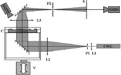
Figure 1: Experimental setup.

The cell is illuminated from below by the expanded collimated beam (pin-hole P1, lenses L1-L2) from the continuous wave laser (CWL). A spatial filter, the lens L3 with 0.1 mm pin-hole P2 at focal distance F=250 mm, rejects all refracted light and forms an image of the anti-nodes on the screen S. Two high-resolution cameras CCD1 and CCD2 (2048 x 2048 pixels) are controlled through the Dantec PIV system. The shutters of both cameras are synchronized in phase with the shaker oscillation. The camera CCD1 collects the images of anti-nodes. Its shatter is open for a time equal to the one period of the parametric wave. The camera CCD2 collects the light scattered by the particles on the surface. It is positioned off axis to avoid straight laser light and its shutter is opened for a shorter time ($\sim$1 ms) to prevent smearing of particle in the images. The CCD2 shutter is opening at the phase when the liquid surface is nearly flat. This allows to keep CCD2 at a minimal angle to the system’s optical axis. The optical axis of CCD2 is perpendicular to the cell long axis.

The measurements of the clustering time as a function of the wave amplitude were performed as follows. For a given cell geometry and chosen frequency, we determined the parametric instability threshold, an oscillation amplitude $A_{c}$. This procedure was similar to that described in SD . Each experimental run has been started from mixing: the shaker amplitude was kept at $A\sim 5A_{c}$ for a couple minutes and then lowered to $A\sim 0.9A_{c}$. Next, a desired amplitude of vibration $A_{i}>A_{c}$ is set and the acquisition of the images from both CCDs started. The unstable parametric wave appears after a time delay with an amplitude growing up to a stationary value proportional $(A-A_{c})^{2}$. A set of collected images always starts from the moment when there are neither waves nor particle motion and ends when a new stationary state reached with the developed wave and clustered particles. After the parametric wave appears, the homogeneous area in CCD1 images is replaced by a network of lines corresponding to the wave anti-nodes (since the water surface curved by the wave serves as a lens). The local line width decreases as the wave amplitude increases, and the maximum of intensity is constant across the line. So the variance of the light intensity averaged over an image area can be chosen as a characteristic of the wave amplitude. The variance of intensity amplitude measured from the particle images (CCD2) represents the amplitude of the growing inhomogeneity in particle concentration. A number of frames collected for each camera is 100 and the frame rate is adjusted using preliminary test runs.

Figure 2a shows the original images of anti-nodes and particle clusters. Figures 2 b,c,d present the results of image processing - the variances of light intensities from CCD1 and CCD2 versus time showing how the particle clustering and the wave develop. The bottom curve 2d shows the wave amplitude taken from CCD1 while the upper two curves, 2b and 2c, present respectively the longitudinal and lateral variances of particle concentration taken from the variances of light intensity measured by CCD2. This allows to observe clustering along each wave vector of the standing wave separately.

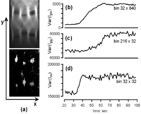
Figure 2: Visualization of the standing wave and particles clustering at the nodes (a), the variance of light intensities as a function of time showing the growth of lateral (b) and longitudinal (c) inhomogeneities in the concentration of particles and the growth of wave amplitude (d)

The time delay between the stabilization of the wave amplitude and the saturation of concentration inhomogeneity is used as a characteristic time of clustering. The inverse clustering time is plotted versus squared wave amplitude in Figure 3. The averaged surface wave amplitude $<A^{2}>$ was determined from the sizes $S_{x},S_{y}$ of the image producing by refracted light in the focal plane P2 of the lens L3. For the refractive index of water 1.33 and small wave amplitudes, the angles $S_{y}/F$ and $S_{x}/F$ are equal to one third of the maximum surface inclination. It follows from Fig. 3 that within 10% the inverse clustering time is proportional to the square of amplitude, as predicted by the theory Nat .

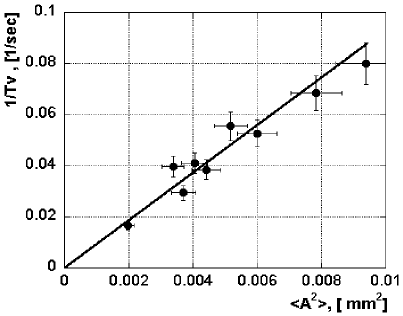
Figure 3: The inverse characteristic time of (lateral) clustering as a function of the squared wave amplitude.

Quasi-linear standing waves exist only at small amplitudes of shaker vibrations. Increasing the amplitude one observes more and more complicated patterns, from spatio-temporal chaos to developed wave turbulence, see e.g. SD ; gollub ; ZLF ; Put ; Cap . Random compressible flows are generally expected to mix and disperse at the scales larger than the correlation scale of the velocity gradients and to produce very inhomogeneous distribution at smaller scales see HH ; FGV ; BFF ; BGH ; BFS ; WG ; BM ; Bruno for theory and gorlum ; Som1 ; Som ; Nam ; alstrom ; CB for experiments. Here we show experimentally that this is also true for a set of random surface waves (for what follows, it is actually enough if particle motion corresponds to so-called Lagrangian chaos). Let us briefly describe relevant mathematical quantities of interest. Consider the number of particles inside the circle of the radius $r$ around the point ${\bf x}$: $n_{r}({\bf x})=\int_{|{\bf r}^{\prime}-{\bf x}|<r}n({\bf r}^{\prime})\,d{\bf r}^{\prime}$. One asks how the statistics of the random field $n_{r}({\bf x})$ changes with the scale of resolution $r$. That can be characterized by the scaling exponents, $\zeta_{m}$, of the moments: $\langle n_{r}^{m}\rangle\propto r^{\zeta_{m}}$. Note that $\zeta_{0}=0$ and $\zeta_{1}=2$. When the distribution is uniform on a surface, one expects $\zeta_{m}=2m$. When this equality breaks for some $m$, one usually calls the distribution fractal. First, the fractal (information) dimension for a random surface flow has been measured by Sommerer and Ott, who found non-integer $d=d\zeta_{m}/dm|_{m=0}$ Som1 . Then, the scaling of the second moment has been found and related to the correlation dimension (again non-integer) Som ; Nam . Therefore, fractality of the distribution has been established in Som1 ; Som ; Nam . To the best of our knowledge, different dimensions have not been compared for the same flow (if found different, that would give a direct proof of multifractality).

On the other hand, a theory recently developed for a short-correlated compressible flow gives the set of exponents BFF ; BGH $\zeta_{m}$ which depend nonlinearly on $m$ (for comparison, note that those theoretical formulas give the Lagrangian exponents which in our notations are $\zeta_{n+1}-2$). Such nonlinear dependence corresponds to a multifractal distribution. Multifractality of the measure predicted in BFF ; BGH means that the statistics is not scale-invariant: strong fluctuations of particle concentration are getting more probable as one goes to smaller scales (increases resolution).

In the second part of the experiment we measured concentration moments and scaling exponents for the suspension of small hydrophilic particles mixed by a surface wave turbulence (at the driving amplitude $\sim 2A_{c}$). Note that at such an amplitude, it is not yet developed turbulence but rather few modes that interact nonlinearly and provide for the Lagrangian chaos. The experiment has been done for a set of oscillation frequencies from 30 to 220 Hz and amplitudes $1.8-2.5A_{c}$. We reproduce here a typical result for the parametric wave with the frequency 32 Hz, wavelength about 7 mm at the oscillation amplitude 198$\mu m\simeq 2A_{c}$. A snapshot of the floaters distribution for this set is shown in Figure 4.

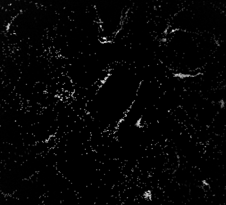
Figure 4: The image of particle distribution in random waves (20 x 20 mm). The number of particles 920.

We checked several approaches to quantify the particle concentration and found that the most reliable algorithm should base on recognition and counting the individual particles. We developed such an algorithm and implemented it for 95 $\mu m$ fluorescent microspheres (No. Duke Scientific Corp.). The particle density is 1.05 g/cm³. To make them floating we used 20% salt (NaCl) solution. Fluorescence method greatly improves the image contrast, eliminates the problem of spurious refractions, and allows positioning the CCD2 camera with an optical filter on the system optical axis. In this part of the experiment we used the cell with the horizontal span 50x50 mm and the depth 10 mm. The size of observation area is about 30x30 mm, the pixel size 15 $\mu m$ and mean particle diameter corresponds to 6-7 pixels.

Images from the experiment with chaotic clustering were preprocessed. A background noise was subtracted using individual threshold for each frame equal to the mean intensity plus 3 standard deviations. The resulted images were smoothed by low-passed 5x5 pixels filter. The particle coordinates were determined maximizing a correlation of 3x3 matrix ($75\times 75\,\mu m$). The method was validated by comparison the number of particles with that estimated on the stage of emulsion preparation. The particle detection in the dense clusters was verified by direct visual inspection of images.

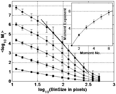
Figure 5: Moments of concentration (2,3,4,5 and 6th) versus the scale of coarse-graining. Inset: scaling exponents of the moments of particle number versus moment number.

Up to 1000 images with particle distributions were recorded at sampling rate 4 sec. The first six moments of the coarse-grained concentration, $N_{m}=\langle n_{r}^{m}\rangle r^{-2m}$, are shown in Figure 5 versus the scale of averaging (bin size $r$). We see that indeed the moments with $m>1$ grow when $r$ decreases below the wavelength of the parametrically excited mode. We see that this growth slows down when $r$ decreases below $r=50$ pixels ($\lg_{1}0(50)\simeq 1.7$). This is possibly due to the dense clusters where the finite particle size, short range repulsion, and the particle back reaction on the flow are important. An additional reason may be an insufficient representation of dense regions by the finite number of particles. On this log-log plot the straight lines correspond to the power laws. The scaling exponents for the interval $50<r<300$ pixels are shown in the inset. The nonlinearity of the dependence of $\zeta$ on $m$ is the first experimental demonstration of multifractality in the distribution of particles.

Another interesting aspect of particle distribution is related to the inertia which may cause particle paths to intersect. This phenomenon was predicted in FFS and called sling effect, it must lead to appearance of caustics in particle distribution WM . At weak inertia (like in our system), caustics are (exponentially) rare FFS ; WM yet we likely see one at the center of Fig. 4. Indeed, as argued in FFS , breakdowns of particle flow are mostly one-dimensional so that caustics must look locally as two parallel straight lines. At higher inertia, breakdowns provide for extra mixing that makes the sum of Lyapunov exponents positive and measure smooth (rather than multi-fractal) Bec ; MW1 . Statistical signatures of co-existence of caustics and multi-fractal distribution needs further studies.

We believe that the new effect of clustering by waves is of fundamental interest in physics and may be of practical use for particle separation, cleaning of liquid surfaces, better understanding of environmental phenomena associated with the wave transport. Chaotic motion of floaters produces the multi-fractal distribution and caustics and is a good model to study behavior of inertial particles in random flows important for water droplets in clouds, fuel droplets in internal combustion engines, formation of planetesimals etc.

The work is supported by the grants of Royal Society, Israel Science Foundation and European network. We thank V. Steinberg for useful discussions. GF is grateful to V. Vladimirov for hospitality and support.

References

- (1) D. Ruelle, J. Stat. Phys. 85, 1 (1996); 86, 935 (1997).
- (2) Balkovsky, E., Falkovich, G. & Fouxon, A. Phys. Rev. Lett. 86, 2790–2793 (2001).
- (3) G. Falkovich and A. Fouxon, nlin.CD/0312033 (2003), New J. of Physics 6, (2004).
- (4) Falkovich, G., Gawedzki, K. & Vergassola, M. Rev. Mod. Phys. 73, 913–975 (2001).
- (5) Ya. G. Sinai, Russian Math. Surveys 27(4), 21–69 (1972).
- (6) R. Bowen and D. Ruelle, Invent. Math. 29, 181 (1975).
- (7) D. Ruelle, J. Stat. Phys. 95, 393 (1999).
- (8) J. R. Dorfman, Introduction to Chaos in Nonequilibrium Statistical Mechanics (Cambridge Univ. Press 1999).
- (9) J.C. Sommerer and E. Ott, Science 259, 335 (1993).
- (10) J.C. Sommerer, Phys. Fluids 8, 2441 (1996).
- (11) A. Nameson, T. Antonsen and E. Ott, Phys. Fluids 8, 2426 (1996).
- (12) J. Cressman and W. Goldburg, J. Stat. Phys. 113, 875 (2003).
- (13) J. Cressman, J. Davoudi, W. Goldburg and J. Schumacher, New Journal Phys. 6, 53 (2004).
- (14) J. Bec, K. Gawedzki, and P. Horvai, Phys. Rev. Lett. 92, 224501 (2004)
- (15) G. Boffetta, J. Davoudi and F. De Lillo, Europhys. Let. (2005).
- (16) G. Falkovich, A. Weinberg, P. Denissenko and S. Lukaschuk, Nature 435, 1045 (2005).
- (17) A. Balk, G. Falkovich and M. Stepanov, Phys. Rev. Lett. 92, 244504 (2004).
- (18) M. Vucelja, in preparation.
- (19) M. Faraday, Phil. Trans. R. Soc. Lond. 121, 319 (1831).
- (20) S. Douady, J. Fluid Mech. 221, 383 (1990)
- (21) B. Gluckman, C. Arnold and J. Gollub, Phys. Rev. E 51 1128 (1995).
- (22) V. Zakharov, V. L’vov and G. Falkovich, Kolmogorov Spectra of Turbulence (Springer-Verlag, Berlin, 1992).
- (23) W. Wright, R. Budakian, D. Pine, and S. Putterman, Science 278, 1609 (1997).
- (24) M. Brazhnikov, G. Kolmakov, A. Levchenko and L. Mezhov-Deglin, Europhys. Let. 58, 510 (2002).
- (25) K. Herterich, and K. Hasselmann, Phys. Oceanography 12, 704 (1982).
- (26) P. Weichman and R. Glazman, J. Fluid Mech. 420, 147 (2000).
- (27) A. Balk and R. McLaughlin, Phys. Lett. A 256, 299 (1999).
- (28) B. Eckhardt and J. Schumacher, Phys. Rev. E 64, 016314 (2001).
- (29) R. Ramshankar, D. Berlin and J. Gollub, Phys. Fluids A 2, 1955 (1990).
- (30) E. Schröder, J. Andersen, M. Levinsen, P.Alstrøm and W. Goldburg, Phys. Rev. Lett. 76, 4717 (1996).
- (31) G. Falkovich, A. Fouxon and M. Stepanov, Nature 419, 151 (2002).
- (32) M. Wilkinson and B. Mehlig, Europhys. Let. 71, 186 (2005).
- (33) J. Bec, J. Fluid Mech. 528 255 (2005).
- (34) B. Mehlig and M. Wilkinson, Phys. Rev. Lett. 92, 250602 (2004).