Present address: ]Department of Physics, Harvard University, Cambridge, Massachusetts 02138 USA

Poisson-to-Wigner crossover transition in the nearest-neighbor spacing statistics of random points on fractals

Abstract

We show that the nearest-neighbor spacing distribution for a model that consists of random points uniformly distributed on a self-similar fractal is the Brody distribution of random matrix theory. In the usual context of Hamiltonian systems, the Brody parameter does not have a definite physical meaning, but in the model considered here, the Brody parameter is actually the fractal dimension. Exploiting this result, we introduce a new model for a crossover transition between Poisson and Wigner statistics: random points on a continuous family of self-similar curves with fractal dimension between 1 and 2. The implications to quantum chaos are discussed, and a connection to conservative classical chaos is introduced.

It is well known that the spectral statistics of almost all quantum systems, whose classical analogs are chaotic, are described quantitatively by Gaussian ensembles of random matrices [1, 2, 3, 4]. Perhaps less well known is the fact that the eigenvalue spacing distribution for the Gaussian orthogonal ensemble of $2\times 2$ random matrices also describes homogeneous Poisson point processes in $\mathbbm{R}^{2}$ [3]. The nearest-neighbor spacing distribution (NNSD) of random points uniformly distributed on a line is given by

$$P_{P}(S)=\exp(-S),$$ (1)

and the NNSD of random points uniformly distributed on a plane is given by [3]

$$P_{W}(S)=\frac{\pi}{2}S\exp\left(-\frac{\pi}{4}S^{2}\right),$$ (2)

which is, in fact, the Wigner distribution of random matrix theory (RMT) [5]. (In Eqs. (1) and (2), $S$ is a dimensionless scaled spacing.) Evidently, random points on a line are uncorrelated, whereas random points on a plane are actually correlated (in the sense that the points tend to avoid each other). Even so, the latter result is reasonable since there is an additional degree of freedom that allows the points to spread out. Based on this intuitive interdependence between “point repulsion” and dimensionality, and in strict analogy to energy-level statistics, it is tempting to indiscriminately conjecture that the nearest-neighbor statistics of random points on a fractal set with noninteger dimension between $1$ and $2$ are described by an intermediate distribution in-between Poisson and Wigner. In fact, this conjecture turns out to be correct as we shall demonstrate below.

Our interest in the nearest-neighbor statistics of random points on fractals was sparked by the provocative results (1) and (2), and the prospect that random points on fractals could be conceptualized as new models of intermediate statistics (between Poisson and Wigner). We however are not the first authors to consider the statistical properties of fractal sets. Two decades ago, Badii and Politi [6] studied (for completely different reasons) the nearest-neighbor distance distribution of random points on a strange attractor. These authors also obtained the probability distribution of nearest-neighbor distances $\delta$ among $N$ points chosen randomly and uniformly on a Cantor set with capacity dimension $D_{0}$. Interestingly, they noted (quite tersely) that the asymptotic distribution (appropriate for large $N$) [6]

$$P_{BP}(\delta,N)=2D_{0}N(2\delta)^{D_{0}-1}\exp\left[-N(2\delta)^{D_{0}}\right],$$ (3)

could be “recognized as a Brody distribution”. Clearly, Eq. (3) is not the Brody distribution [7], but we show that when the nearest-neighbor distance is rescaled by the mean nearest-neighbor distance (which is a contrivance familiar to practitioners of RMT) the result is indeed the Brody distribution. More generally speaking, we show that the Brody distribution is the NNSD for points selected uniformly at random from a self-similar set $K\subset\mathbbm{R}^{d}$ with similarity dimension $d_{s}\geq 1$, and that the Brody parameter is the (relative) similarity dimension of $K$ (i.e. $d_{s}-1$). (In this paper, $d$ is the Euclidean space dimension.) The goals of this paper are to derive this result, to introduce a new model for a Poisson-to-Wigner crossover transition based on this result, and to explicate the physical implications. The derivation is simple and direct; the result itself is far more interesting than its proof. A discussion of the physical implications is deferred to the conclusion.

We begin first with the derivation of the spacing distribution. Suppose that $N$ points of a self-similar set $K\subset\mathbbm{R}^{d}$ are chosen randomly and uniformly. The probability $P(s)\text{d}s$ of finding the nearest neighbor to a given point at a distance between $s$ and $s+\text{d}s$ is equal to the probability of finding one of the $(N-1)$ points at a distance between $s$ and $s+\text{d}s$ from the given point and the $(N-2)$ remaining points at a distance greater than $s$. Let $\mathpzc{P}(s)$ denote the probability of finding a point within a distance $s$ of a given point. The probability of finding one point at a distance greater than $s$ is then $(1-\mathpzc{P}(s))$, and for $(N-2)$ points, the probabilities are multiplicative due to the fact that all points are chosen independently. Thus,

$$P(s)\text{d}s=\eta\left(1-\mathpzc{P}(s)\right)^{(N-2)}\text{d}\mathpzc{P}(s),$$ (4)

where the prefactor $\eta=(N-1)$ accounts for the fact that the nearest neighbor could be any one of the $(N-1)$ points , and $\text{d}\mathpzc{P}(s)=\mathpzc{P}^{\prime}(s)\text{d}s$ is the probability of finding a point in a shell with inner and outer radii $s$ and $s+\text{d}s$ centered about the given point. The probability of finding multiple nearest neighbors is ignored since the probability of such an event is higher order in $\text{d}s$ and is therefore insignificant compared to the probability of finding a single nearest neighbor.

It now remains to specify the probability $\mathpzc{P}(s)$. Clearly, the typical number of neighbors of a given point will vary more rapidly with distance from that point as the dimension increases. The probability $\mathpzc{P}(s)$ is, by definition, the ratio of the number of points within some prescribed distance to the total number of points, that is, $\mathpzc{P}(s)=N(s)/N(\mathcal{R})$, where $\mathcal{R}$ is the radius of the $d$-dimensional ball that contains all $N$ points. The number function $N(s)$ can be directly obtained from the so-called “mass-radius scaling law” for fractals (see page 40 of Mandelbrot’s book [8]): $M(r)=M(\mathcal{R})(r/\mathcal{R})^{D_{m}}=[M(\mathcal{R})/\mathcal{R}^{D_{m}}]r^{D_{m}}$. In this formula, $M(r)$ and $M(\mathcal{R})$ are the masses contained within balls of radii $r$ and $\mathcal{R}$, respectively, and $D_{m}$ is the mass dimension. For regular (i.e. strictly self-similar) fractals, $D_{m}=d_{s}$. It might seem peculiar to speak of masses here, but it is equivalent to the concept of numbers of points within balls of a specified radius if an individual sample point becomes the unit of mass. We can thus equitably think of the above mass law as a “number-radius scaling law”. So, the probability of finding a point within a distance $s$ of a given point is governed by the power law

$$\mathpzc{P}(s)=As^{d_{s}},$$ (5)

where the coefficient $A=1/\mathcal{R}^{d_{s}}$, and $d_{s}\geq 1$ is the similarity dimension of $K$. (Note that the probability $\mathpzc{P}(s)$ is a unitless number since $A$ has units of $1/(\text{length})^{d_{s}}$.) Therefore, Eq. (4) becomes

$$P(s)\text{d}s=\eta\left(1-As^{d_{s}}\right)^{(N-2)}Ad_{s}s^{d_{s}-1}\text{d}s.$$ (6)

Recall that $\text{d}\mathpzc{P}(s)=\mathpzc{P}^{\prime}(s)\text{d}s=Ad_{s}s^{d_{s}-1}\text{d}s$. It is straightforward to verify that the probability density $P(s)$ is already normalized (i.e. $\int_{0}^{\mathcal{R}}P(s)\text{d}s=1$). We could now consider the large $N$ limit of Eq. (6), and in doing so, we can invoke the so-called Poisson approximation , and this gives the asymptotic probability density

$$P(s)=NAd_{s}s^{d_{s}-1}\exp\left(-NAs^{d_{s}}\right)\quad\text{as}~{}N\rightarrow\infty.$$ (7)

Equation (7) is essentially the distribution obtained by Badii and Politi in 1985 (c.f. Eq. (3) and note that $D_{0}$ in their formula is equivalent to $d_{s}$ in Eq. (7)).

Next, we calculate the mean spacing $\bar{s}=\int_{0}^{\mathcal{R}}sP(s)\text{d}s$:

$$\bar{s} = {(N-1)d_{s}\over\mathcal{R}^{d_{s}}}\int_{0}^{\mathcal{R}}s^{d_{s}}\left(1-\left({s\over\mathcal{R}}\right)^{d_{s}}\right)^{(N-2)}\text{d}s$$

$$= \mathcal{R}(N-1)d_{s}\int_{0}^{1}u^{d_{s}}\left(1-u^{d_{s}}\right)^{(N-2)}\text{d}u$$

$$= \mathcal{R}(N-1)\int_{0}^{1}v^{1/d_{s}}(1-v)^{(N-2)}\text{d}v$$

$$= \mathcal{R}(N-1)B\left(1+{1/d_{s}},N-1\right)$$

$$= \mathcal{R}\Gamma(N)\Gamma\left(1+{1/d_{s}}\right)/\Gamma\left(N+{1/d_{s}}\right).$$

In the second line, we have made a change of variables $u=s/\mathcal{R}$, and in the third line, we have made one further change of variables $v=u^{d_{s}}$. The integral in the third line we recognize as the Beta function $B(\mu,\nu)$ with parameters $\mu=1+1/d_{s}$ and $\nu=N-1$, and this then gives the fourth line. We then used the usual relation between the Gamma and Beta functions to arrive at the fifth line. It can be shown that the term

$${\Gamma(N)\over\Gamma\left(N+{1/d_{s}}\right)}={1\over N^{1/d_{s}}}\left(1+O\left({1\over N}\right)\right)\quad\text{as}~{}N\rightarrow\infty,$$ (8)

and therefore, the asymptotic mean nearest-neighbor spacing is, to leading order,

$$\bar{s}={\mathcal{R}\over N^{1/d_{s}}}~{}\Gamma\left({d_{s}+1\over d_{s}}\right)\quad\text{as}~{}N\rightarrow\infty.$$ (9)

Introducing the rescaled spacing $S={s/\bar{s}}$ and taking the limit $N\rightarrow\infty$, the distribution $P(s)$ in Eq. (7) becomes the distribution

$$P_{B}(S;q=d_{s}-1)=\alpha d_{s}S^{d_{s}-1}\exp\left(-\alpha S^{d_{s}}\right),$$ (10a)

where

$$\alpha=\left[\Gamma\left(\frac{d_{s}+1}{d_{s}}\right)\right]^{d_{s}}.$$ (10b)

(Notice that the rescaling of $s$ by $\bar{s}$ was doubly beneficial; both explicit dependences on $\mathcal{R}$ and $N$ in Eq. (7) have been removed.) The distribution $P_{B}(S;q)$ [Eq. (10)] is, in fact, the Brody distribution [7] with Brody parameter $q$ equal to $d_{s}-1$ . We refer to the number $d_{s}-1$ as the relative similarity dimension of $K$ since this number is the difference between the similarity dimension of $K$ and the similarity dimension of a line (the simplest self-similar object) which is equal to $1$. Equation (10) is valid for random points on any self-similar subset of $\mathbbm{R}^{d}$ with similarity dimension $d_{s}\geq 1$. If $K$ is a classical (nonfractal) self-similar set (i.e. a $d$-dimensional cube), then $d_{s}=d$ and Eq. (10) reduces to the NNSD for a homogeneous Poisson point process in $\mathbbm{R}^{d}$ (see Ref. [3]).

In studies of quantum chaos, the Brody distribution has sometimes been used (as a purely phenomenological distribution) to describe the nearest-neighbor energy-level statistics of quantum systems that undergo a direct transition from Poisson-like to Wigner-like statistics as a system parameter is varied. (A classic example is the diamagnetic Kepler system [9].) In the present context, a Poisson-to-Wigner transition can be realized by considering point processes on a family of self-similar sets whose dimension ranges between $1$ and $2$ as some set parameter is varied. In actual fact, we are introducing a new model (that does not involve random matrices) for a Poisson-to-Wigner crossover transition, and this model is special since the intermediate statistics are described exactly by the Brody distribution. As a concrete example, we now study point processes on the family of Koch fractals in $\mathbbm{R}^{2}$. These fractals can be thought of as the attractors of a one-parameter family of iterated function systems (IFSs). The similarity transformations defining the IFS involve a rotation which is conveniently parametrized by the angle $\theta$. When $\theta=0$, the attractor is a line, and when $\theta=\pi/2$, the attractor is the famous Sierpinski-Knopp plane-filling curve, whose image is a solid isosceles triangle in $\mathbbm{R}^{2}$ [10]. For intermediate values [i.e. $\theta\in(0,\pi/2)$], the attractors are various self-similar curves of prescribed dimension $d_{s}\in(1,2)$. The nearest-neighbor statistics of the random points undergo a continuous transition from Poisson to Wigner statistics (see Fig. 1) as the self-similar set continuously deforms from a line to a plane-filling curve (i.e. as the rotation angle $\theta$ varies between $0$ and $\pi/2$).

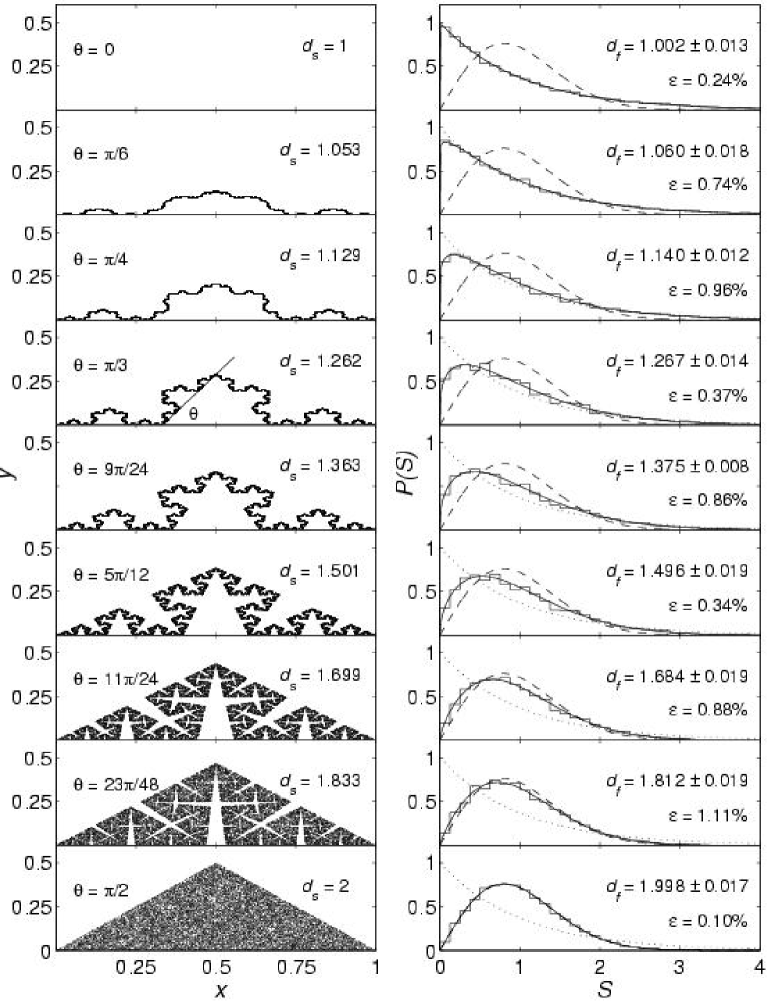
Figure 1: A crossover transition between Poisson and Wigner statistics resulting from point processes on the family of Koch fractals in $\mathbbm{R}^{2}$. The left panel shows random points on several fractals that belong to the family (each one specified by a particular choice of the rotation angle $\theta$). The exact similarity dimension $d_{s}$ of each of the fractals (given to three decimal places) is indicated on each window. The right panel shows the corresponding NNSD of the points on each fractal. The numerical data (i.e. $d_{f}=\bar{d}_{f}\pm\sigma$ and $\varepsilon$) indicated on each window are as described in the text. The dotted, dashed, and solid curves are the distributions $P_{P}(S)$, $P_{W}(S)$, and $P_{B}(S;\bar{d}_{f}-1)$, respectively.

For clarity, we mention some pertinent numerical details. Random points on these fractals were selected using the random iteration algorithm (RIA) [11]. The distance between a given point $\mathbf{x}_{i}$ and its nearest neighbor is defined (using the Euclidean metric) by $s_{i}=\text{min}\left\{\sqrt{(x_{i}-x_{j})^{2}+(y_{i}-y_{j})^{2}}\right\}$ for $i,j=1,\ldots,N$ ($j\neq i$). Although $\{s_{i}\}$ define a set of spacings, the NNSD is actually defined in terms of the scaled spacings $S_{i}=s_{i}/\bar{s}$, where $\bar{s}={1\over N}\sum_{i=1}^{N}s_{i}$, is the (numerically-calculated) mean nearest-neighbor spacing. We constructed the histograms by binning all values of $S_{i}$ and then normalizing the area under the histogram to unity. Each histogram was constructed from one sample of $N=20~{}000$ random points. We mention here that by using all of the points selected by the RIA in the statistical analysis, we introduce some error due to finite-size or edge effects. These errors are statistically insignificant as long as $N$ is sufficiently large (see Eq. (9)). Although not absolutely necessary, we use the Levenberg-Marquardt method [12] to determine the numerical value of the parameter $d_{s}$ that gives the optimal fit of the Brody distribution $P_{B}(S;d_{s}-1)$ to the histograms. This number $d_{f}$ can then be immediately compared to the theoretical value. The purpose of this procedure is to test how accurately the Brody distribution [Eq. (10)] reproduces the histogram data obtained from particular realizations of the model. Of course, each realization (in general) yields a unique histogram (and hence a unique $d_{f}$), and so it is more informative to average over several (say $n$) realizations and subsequently define $d_{f}=\bar{d}_{f}\pm\sigma$, where $\bar{d}_{f}$ is the average $d_{f}$ value obtained from the $n$ realizations and $\sigma$ is the standard deviation. The percentage error (denoted by $\varepsilon$) of $\bar{d}_{f}$ (obtained from $n=10$ independent realizations) relative to $d_{s}$ is typically under $1\%$. We have in fact studied point processes on many of the well-known classical fractals in $\mathbbm{R}^{2}$, $\mathbbm{R}^{3}$, and $\mathbbm{R}^{4}$ , and in almost all cases the accuracy is comparable.

The nearest-neighbor energy-level statistics of some quantum systems execute a Poisson-to-Wigner transition as the underlying classical dynamics monotonically change from being completely integrable to completely chaotic. One example is the family of Robnik billiards [13]. A monotonic transition between integrabililty and chaos is however quite exceptional. More typically, the degree of “chaoticity” of the classical dynamics (as measured by the volume fraction of phase space filled with chaotic trajectories) changes in a complicated way as a system parameter is varied monotonically, and so the energy-level statistics will not undergo a direct transition from Poisson to Wigner. For example, the energy-level statistics of the hydrogen atom in a van der Waals potential undergo a Wigner-Poisson-Brody-Poisson-Brody-Poisson-Wigner transition as the appropriate system parameter is monotonically varied in a specified range [14]. Regardless, in the intermediate regime between integrability and hard chaos, the Brody distribution (albeit a pure surmisal) has often been found to be a good delineation of the energy-level spacing histogram. There are, in fact, systems for which the statistical confidence is high (an example is the ripple billiard [15]). This is not to say the Brody distribution is now established as a distribution that quantitatively describes energy-level statistics in the intermediate regime, but rather that after 30 years of pervasive use with considerable success, the Brody distribution has garnered an undeniable phenomenological significance. (Of course, other distributions have been proposed and used to interpolate between the Poisson and Wigner limits; we cite here a few of the more popular distributions [16, 17, 19, 18, 20]. These efforts cannot be disregarded, but they are not directly relevant to the present discussion.) Given our present result and the phenomenological status of the Brody distribution in studies of quantum chaos, there is a profound implication that transpires: Phenomenologically, the energy levels of a typical time-reversal invariant quantum system, whose dynamics in the classical limit are mixed, have the same nearest-neighbor statistics as random points on a fractal with dimension in-between $1$ and $2$. This phenomenological corollary, together with analogous corollaries in the limiting cases of integrability [Eq. (1)] and hard chaos [Eq. (2)], offer a new phenomenology for quantum chaos: the nearest-neighbor energy-level statistics of a typical time-reversal invariant quantum Hamiltonian follow the statistics of (i) random points on a (one-dimensional) line if the classical limit is integrable; (ii) random points on a (two-dimensional) plane if the classical limit is fully chaotic; and (iii) random points on a fractal set with dimension in-between $1$ and $2$ if the classical limit is mixed.

This phenomenological behavior is quite puzzling. Why should the energy levels of a quantum Hamiltonian behave (insofar as their nearest-neighbor statistics) like random points on a fractal or on a plane? This is a very difficult question to answer since there is no direct connection between point processes and quantum mechanics. Point-process models (PPMs) and random-matrix models are both stochastic models, but unlike random-matrix models, PPMs do not inherently contain any of the structure of quantum mechanics, and so it is difficult to understand why point-process statistics should have any relation to energy-level statistics. Surreptitiously, the fundamental link is classical mechanics. The model of random points on a fractal can be regarded as a simple stochastic model for chaotic dynamics on a Poincaré section. In mixed Hamiltonian systems, regular and chaotic regions are comingled, and the chaotic regions, in particular, are fractal in nature. If we restrict our scope (at least initially) to two-degree-of-freedom billiard systems (such as the family of Robnik billiards), then we know that the chaotic trajectories explore (in a seemingly random fashion) a fractal subset of the Poincaré section having dimension in-between 1 and 2. Clearly, the NNSD of the “chaotic points” on the section (corresponding to a chaotic trajectory) must be Poisson-like in the near-integrable regime, Wigner-like in the chaotic regime, and some intermediate distribution in-between Poisson and Wigner in the mixed regime. The intermediate distribution must also have built in point repulsion. If random points on fractal sets embedded in $\mathbbm{R}^{2}$ really are apt models of Hamiltonian chaos (on a Poincaré section), then the intermediate distribution should be the Brody distribution. If so, then there is an even deeper corollary: Phenomenologically, the energy levels of a typical time-reversal invariant quantum system (whose classical analog is nonintegrable) have the same nearest-neighbor statistics as the chaotic trajectories of the underlying classical Hamiltonian. Of course, we have not explicitly demonstrated that PPMs correctly describe the nearest-neighbor statistics of chaotic trajectories, and we can only begin to do so through numerical experiments. This shall be the subject of a future paper. The purpose of the above discussion was merely to introduce the idea of linking PPMs with classical mechanics, and to outline one of the potential implications. For the present, we must settle for the less fundamental, but nonetheless far-reaching precursor (italicized above).

References

- [1] O. Bohigas, in Chaos and Quantum Physics, edited by M.-J. Giannoni, A. Voros, and J. Zinn-Justin (North-Holland, Amsterdam, 1991).
- [2] H.-J. Stöckmann, Quantum Chaos: An Introduction (Cambridge University Press, Cambridge, 1999).
- [3] F. Haake, Quantum Signatures of Chaos, Second Edition (Springer, Berlin, 2001).
- [4] L. E. Reichl, The Transition to Chaos in Conservative Classical Systems: Quantum Manifestations, Second Edition (Springer, New York, 2004).
- [5] M. L. Mehta, Random Matrices, Third Edition (Elsevier, San Diego, 2004).
- [6] R. Badii and A. Politi, J. Stat. Phys. 40, 725 (1985).
- [7] T. A. Brody, Lett. Nuovo Cimento 7, 482 (1973); T. A. Brody et al., Rev. Mod. Phys. 53, 385 (1981).
- [8] B. B. Mandelbrot, The Fractal Geometry of Nature (W. H. Freeman and Company, San Francisco, 1982).
- [9] D. Wintgen and H. Friedrich, Phys. Rev. A 35, 1464 (1987).
- [10] H. Sagan, Space-Filling Curves (Springer-Verlag, New York, 1994).
- [11] M. F. Barnsley, Fractals Everywhere, Second Edition (Academic Press, Boston, 1993).
- [12] W. H. Press et al., Numerical Recipes in C: The Art of Scientific Computing, Second Edition (Cambridge University Press, Cambridge, 1992).
- [13] T. Prosen and M. Robnik, J. Phys. A 26, 2371 (1993); ibid. 27, 8059 (1994).
- [14] K. Ganesan and M. Lakshmanan, Phys. Rev. A 48, 964 (1993).
- [15] W. Li, L. E. Reichl, and B. Wu, Phys. Rev. E 65, 056220 (2002).
- [16] M. V. Berry and M. Robnik, J. Phys. A 17, 2413 (1984).
- [17] F. M. Izrailev, J. Phys. A 22, 865 (1989).
- [18] E. Caurier, B. Grammaticos, and A. Ramani, J. Phys. A 23, 4903 (1990).
- [19] G. Lenz and F. Haake, Phys. Rev. Lett. 67, 1 (1991).
- [20] C. I. Barbosa et al., Phys. Rev. E 59, 321 (1999).