Low-dimensional chaos in populations of strongly-coupled noisy maps

Abstract

We characterize the macroscopic attractor of infinite populations of noisy maps subjected to global and strong coupling by using an expansion in order parameters. We show that for any noise amplitude there exists a large region of strong coupling where the macroscopic dynamics exhibits low-dimensional chaos embedded in a hierarchically-organized, folded, infinite-dimensional set. Both this structure and the dynamics occuring on it are well-captured by our expansion. In particular, even low-degree approximations allow to calculate efficiently the first macroscopic Lyapunov exponents of the full system.

1 Introduction

It has now been some fifteen years since the discovery of collective behavior emerging out of infinite populations of incoherent nonlinear/chaotic units. In many instances, collective cycles have been found and studied, especially in locally-coupled, spatially-extended systems. Although originally discussed rather early [1],  robust nontrivial collective chaos has been documented only in the case of globally-coupled populations,[2, 3, 4, 5, 6, 7]  and the nature and dimensionality of this chaos is still a matter of debate[8, 9]. Indeed, many intermediate situations have been uncovered between the infinite-dimensional chaos of weakly-coupled units and the low-dimensional chaos of the fully synchronized regimes occurring in the strong coupling limit.

The effect of microscopic noise on such systems is a rather new topic of investigation.[10, 11] Concerning collective chaos, Shibata et al.[10] showed that its dimensionality can be drastically reduced by microscopic noise added to populations of weakly-coupled chaotic maps. Here we approach the same issue, starting from the fully-synchronized, strong-coupling limit. We have shown recently[12] that this trivial collective chaos can be unfolded by the action of noise, allowing extra degrees of freedom to perturb the macroscopic dynamics. Starting from the fully-synchronized noiseless regime, we study in some detail the apparently low-dimensional chaotic regimes appearing when the noise intensity is increased.

This paper follows a series of previous works in which, in particular, we have introduced a systematic order parameter expansion which approximates with increasing accuracy the macroscopic dynamics observed at strong coupling values by low-dimensional effective maps for a small set of macroscopic observables[13, 14, 15]. Here we use this expansion scheme to tackle the issue of the actual dimensionality of the collective chaos observed.

In the following section, we present numerical simulations illustrating the emergence of deterministic collective behavior in the infinite-size limit and briefly review the order parameter expansion by which we can approximate the macroscopic dynamics through a set of hierarchically-organized low-dimensional systems. We then explore some consequences of such a representation in the case of maximal coupling. Notably, we show how different microscopic features, such as the shape of the noise distribution or the nonlinearity of the individual dynamics, translate into the collective bifurcation diagram.

In the remaining of the paper, we address the question of the nature and extent of the information about the collective behavior that we can extract from our low-dimensional approximations.

In Section 3, we show that the macroscopic attractor has a folded structure that is organized with the same hierarchy as our order parameters: the attractor is an infinitely-folded object whose folds on a smaller scale are captured by order parameters of increasing degree.

In Section 4, we show that the hierarchy of the reduced systems also reflects the order in which the macroscopic degrees of freedom emerge and determine the collective dynamics. The reduced systems reproduce the dominant exponents of the Lyapunov spectrum for the population, as computed from the so-called “nonlinear Perron-Frobenius operator”.[16, 17, 18, 19] In particular, we show that, in the region of interest, collective chaos is characterized by only one positive Lyapunov exponent, while the other macroscopic degrees of freedom play the role of fast modes with negative associated Lyapunov exponents. Nevertheless, the dimension of the attractor, as measured by the Lyapunov dimension, can increase when the magnitude of the negative eigenvalues reduces. This typically happens when the coupling is weakened.

In the last section, we discuss the perspectives of our work and in particular the region of intermediate couplings and weak noise, where the collective dynamics is high dimensional also in the noiseless case and the order parameter expansion to low degree diverges.

2 Macroscopic dynamics

2.1 Order parameter expansion

We address here the population of globally-coupled noisy maps:

$$x_{j}\mapsto(1-K)\,f(x_{j})+K\,\langle\,{f(x)}\,\rangle+\xi_{j}(t)\quad j=1,\dots N,$$ (1)

where $f:\mathbb{R}\rightarrow\mathbb{R}$ defines the individual (local) dynamics, $K\in[0,1]$ quantifies the coupling of every population element to the average iterate $\langle\,{f(x)}\,\rangle$ and $\xi_{j}(t)$ is an independent noise term, drawn according to a given distribution of finite moments $m_{q}$. The collective dynamics is addressed, without loss of generality, in terms of the evolution of the simplest macroscopic variable, i.e. the average population state or mean field:

$$X=\langle\,{x}\,\rangle=\frac{1}{N}\sum_{j=1}^{N}x_{j}.$$ (2)

Numerous studies of the noiseless case have revealed that the mean field of such a population can display a wealth of dynamical regimes, ranging from one-dimensional chaos for strong coupling, when full synchronization is attained, to higher dimensional chaos in the clustering region (the dimensionality depending on the number of clusters). [20, 16, 21, 22, 17, 23, 24, 7, 25, 26, 27, 28]

The addition of noise to this system —as well as parameter diversity— has been often conceived as a means of testing the genericity of the aforementioned results and the structural stability of the collective dynamics.[17]  Another approach consists in fixing the parameters of the individual map and systematically vary the noise intensity. Changing the variance of the noise distribution has revealed that the stochastic terms interact with the nonlinearities of the dynamical system. For large populations, noise affects the high dimensional collective dynamics at low coupling by reducing the dimensionality of the turbulent motion.[10]

In spite of the trivial simplicity of the macroscopic dynamics in the fully synchronous regime, the modifications of the collective behavior induced by noise are far from straightforward. For instance, as shown by Kuramoto and Teramae, even weak noise can cause the population distribution moments to scale anomalously with respect to the noise distribution moments over a range of scales.[11, 15]

In recent work, we have focused on how the addition of noise to a synchronous regime modifies the collective dynamics.[12, 15]  Somewhat counterintuitively, although noise blurs the trajectory of any population element, it affects the mean field of infinite populations in a deterministic way. This is because, in the limit of infinite population size, the macroscopic dynamics is the result of the averaging of infinitely-many independent stochastic processes. More surprisingly, the macroscopic attractor still appears low-dimensional even away from the full-synchronization regime.

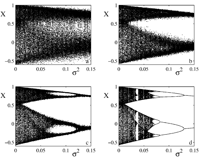
Figure 1: Bifurcation diagrams of the mean field Eq. (2) for $K=1$ and populations of increasing size $N$: a) $N=10^{2}$ b) $N=10^{3}$ c) $N=10^{4}$ d) $N=10^{6}$ and reduced system. The noise intensity $\sigma^{2}$ plays the role of control parameter, while the parameters of the local dynamics Eq. (3) are kept fixed.

As an illustrative example, we consider now a population governed by Eq. (1), where

$$f(x)=1-a\,x^{2}$$ (3)

is a chaotic logistic map ($a=1.57$, one-band chaos) and the noise distribution is taken uniform. Varying the variance of the noise distribution $\sigma^{2}$ as a control parameter, a deterministic bifurcation diagram emerges when the population size $N$ is increased (Fig. 1).

We recently introduced an order parameter expansion, which allows to approximate, in the strong-coupling region, the deterministic collective dynamics by means of a low-dimensional map.[12]  This macroscopic effective dynamical system is obtained by writing the evolution equation for the mean field $X$ as coupled to other macroscopic variables, or order parameters:

$$\Omega_{q}:=\langle\,{\epsilon^{q}}\,\rangle\hskip 56.9055ptq\in\mathbb{N},$$ (4)

where $\epsilon_{j}=x_{j}-X$ is the deviation of a population element from the mean field. In this case, Eq. (4) identifies the moments of the population distribution at a fixed time instant. The infinite-dimensional map defining the evolution of all such order parameters is formulated in powers of $(1-K)$, so that a truncation to a given degree $n$ provides a reduced system of dimension $n$ which reads:

$$\begin{cases}X\mapsto&f(X)+\sum_{q=2}^{n}\>A_{q}(X)\Omega_{q}\\ \rule[0.0pt]{0.0pt}{19.91692pt}\Omega_{q}\mapsto&m_{q}+\sum_{i=1}^{q}\binom{q}{i}(1-K)^{i}\,m_{q-i}\,\Gamma_{i}(X,\Omega_{2},\dots\Omega_{n})\hskip 19.91692ptq=2,\dots n\end{cases}$$ (5)

where $A_{q}$ and $\Gamma_{i}$ depend on the first $2P$ moments of the noise distribution.[15] Of the remaining order parameters, those up to $q=n\,P$ ($P$ being the degree of the the map $f$) have a dynamics slaved to the the first $n$, while the others are constantly equal to the noise distribution moment of corresponding order.

In the Appendix, we write the reduced systems up to the fourth degree when the logistic map Eq. (3) defines the individual dynamics. There, the $A_{q}$ and $\Gamma_{i}$ are explicitly derived as functions of the first order parameters.

The population-level parameters that figure in Eqs. (5) are those of the individual map, defining its degree of nonlinearity, the moments $m_{q}$ of the noise distribution, and the coupling constant $K$. The noise variance $\sigma^{2}$, that we typically choose as the bifurcation parameter, hence appears naturally as one of the parameters of the macroscopic description.

2.2 Interplay of map nonlinearities and noise moments

One first consequence of representing the macroscopic dynamics by means of Eqs. (5) is that we can disentangle the effects of the local nonlinearities from those of the noise. Let us consider the case of maximal coupling $K=1$. Here, the zeroth-degree representation for $n\rightarrow\infty$ is exact and takes the form:

$$X\mapsto f(X)+\sum_{q=1}^{\infty}\>\frac{1}{q!}\>\mathcal{D}^{q}f(X)\>m_{q},$$ (6)

where $\mathcal{D}^{q}f$ is the $q$-th derivative of the individual map.

When noise is added, the uncoupled map is perturbed by a term where the moments of the noise distribution are weighted by the nonlinearities of the map. Any (polynomial) map of maximal degree of nonlinearity $p$ will only be influenced by the first $p$ moments of the noise distribution. As a consequence, in the case of quadratic maps such as the logistic one, the macroscopic dynamics will be affected in the same way by any noise distribution of given variance and is described by:

$$X\mapsto 1-a\>\sigma^{2}-a\>X^{2}.$$ (7)

This is, of course, another logistic map which can be rescaled to the uncoupled one via a simple change of variables (see Fig. 1(d) for its bifurcation diagram, overlapping, up to finite-size effects, that of the full population).

In order to explore how the macroscopic dynamics is affected by noises of the same intensity (defined as the variance $\sigma^{2}$ ), but whose distributions have otherwise different features, the individual map needs to have nonlinearities of order higher than two. Consider, for example, the quartic map defined by a perturbation of the previously considered logistic equation:

$$x\mapsto 1-a\,x^{2}+b\,x^{4},$$ (8)

where $a=1.57$ and $b=0.1$. For these parameter values, the quartic map is chaotic.

The reduced system Eq. (6) reads in this case:

$$X\mapsto 1-a\,\sigma^{2}+b\,m_{4}-\left(a-6\,b\,\sigma^{2}\right)\,X^{2}+b\>X^{4}.$$ (9)

which is another quartic map, whose bifurcation diagram is shown in Figure 2(a) for uniform and Gaussian noise distributions. The order parameter expansion reproduces the interaction of the single-element nonlinearities with the noise distribution features.

The effect on the collective dynamics of an increase in the noise intensity allows us to distinguish, on a purely macroscopic basis, between microscopic stochastic processes with differences in the moments up to the fourth one. The distance between the dynamics induced by the two noise distributions are larger for larger noise intensity. Strikingly, the collective dynamics is either chaotic or stationary for strong noise. Figure 2 also shows that the macroscopic dynamics is bistable for intermediate noise values and that the hysteresis region is slightly changed by the kind of noise that is applied. Similar hysteretical phenomena have been also observed in populations of globally coupled ODEs with independent noise,[29]  and find here a simple origin within our approach.

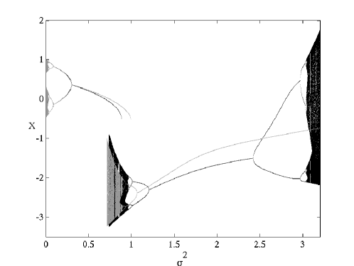
Figure 2: Bifurcation diagrams of Eq. (9) for a local dynamics defined by Eq. (8) with different noise distributions: Gaussian (grey), uniform (black). The diagrams are indistinguishable, up to finite-size effects, from those of the corresponding population.

For any polynomial of $P$-th degree, the macroscopic dynamics at maximal coupling will be exactly described by a polynomial of the same order, whose parameters are the first $2P$ moments of the noise distribution. If the uncoupled map is not polynomial, in principle all the noise distribution moments affect the macroscopic dynamics and Eq. (6) might be a diverging series. In some cases, however, the fact that $m_{q}$ scales as $\sigma^{q}$ allows to approximate the series by its truncation to a finite degree in $\sigma$. As long as noise is sufficiently weak, a formal truncation to a sufficiently high degree is able to describes in detail the macroscopic bifurcation diagram of the full system. For instance, this applies to population of excitable maps, where microscopic noise gives rise to complex collective behavior.[12, 30]

3 Fine structure of the macroscopic attractor

When $K<1$, the zeroth-degree reduced system is no longer an exact solution for the collective dynamics, but Eq. (5) provides a hierarchy of maps ordered in powers of $(1-K)$. For not too small coupling values, the macroscopic dynamics still looks rather low-dimensional. As we have shown already in Refs. demonte04 and demonte05, this hierarchy, when truncated, can account quantitatively for the collective dynamics. The rest of this paper is dedicated to explore in some detail what are the characteristics of the macroscopic dynamics that are captured by such low-dimensional systems. In particular, we will address what changes in the mean field attractor are induced by a reduction of the coupling strength $K$.

Figure 3 displays a bifurcation diagram for fixed noise intensity and varying coupling strength. As for the case, illustrated in Fig. 1 (d), of fixed $K$ and varying $\sigma^{2}$, the collective dynamics seems to undergo macroscopic bifurcations among low-dimensional regimes. However, the scaling in the width of the chaotic bands and the distribution of the periodic windows suggests that the diagram might not be straightforwardly rescaled to that of the local scalar map. The anomalies become more evident when the noise intensity is weakened: for instance, for low coupling the macroscopic dynamics enters a region of multistability, probably associated with the presence of clusters in the limit of zero noise.

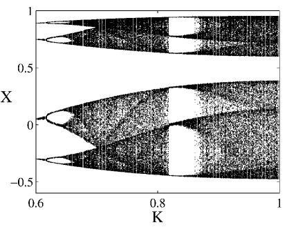
Figure 3: Bifurcation diagram with respect of the coupling strength $K$ for the mean field of a population of $N=2^{20}$ globally coupled logistic maps with added microscopic uniform noise of variance $\sigma^{2}=0.03$.

In this Section, we study the structure of the macroscopic attractor and compare the simulations for the full system to those of the reduced systems to the first four degrees. As a case study, we choose the population of logistic maps whose local dynamics is defined by Eq. (3) and a uniform distribution for the noise term. The reduced systems relative to this population are given in the Appendix.

Let us start by considering the first return map of the mean field. When the coupling is maximal, the mean field evolves according to the one-dimensional map Eq. (7). Its first return map hence lies onto a one-dimensional manifold, the parabola:

$$X(t+1)=1-a\>\sigma^{2}-a\>X^{2}(t).$$ (10)

Reducing the coupling, this parabola folds (Fig. 4(a)), which indicates that the macroscopic attractor is no longer strictly one-dimensional. Eq. (7) is not able to account for the modification of the attractor, but the folding is captured with great accuracy by the reduced system of second degree Eq. (14).

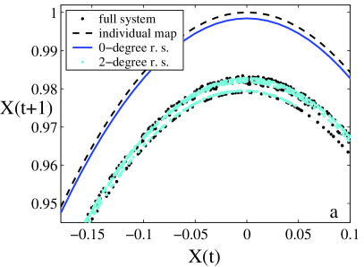
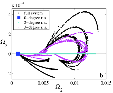
Figure 4: a) First return map for the mean field of the population (black dots) and for the reduced system of second degree Eq. (14) (grey dots), for $K=0.4$ and $\sigma^{2}=0.001$. The dashed line is the invariant parabola Eq. (10) where the single-element dynamics is embedded, the solid line is the invariant parabola for the zeroth-degree approximation Eq. (7). b) The third order parameter $\Omega_{3}$ versus the second $\Omega_{2}$ for the population of logistic maps (black dots) and for the third degree reduced system Eq. (16). The continuous line is the invariant manifold which embeds the dynamics of Eq. (14) and of Eq. (7) (square).

In spite of the fact that the reduced system of second degree reproduces qualitatively and quantitatively the macroscopic dynamics of the population, this approximation is not able to track modifications of the mean field attractor related to the asymmetry of the population distribution around its average. Such asymmetry appears as the coupling is less than maximal, and is best revealed by looking at the third order parameter $\Omega_{3}$ as a function of the second order parameter $\Omega_{2}$ (Fig. 4 (b)). In the zeroth and second-order approximations, the dynamics of $\Omega_{2}$ is restricted to the line $\Omega_{3}=0$, and in the first case it reduces to the trivial fixed point $(\sigma^{2},m_{3})$ of Eq. (7). The reduced system of third degree is a three-dimensional map, reported in Appendix, for the mean field, the second and the third order parameter. Figure 4 (b) shows that, contrary to the lower degree truncations, it gives rise to the same folding observed for the population third moment.

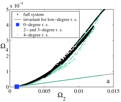
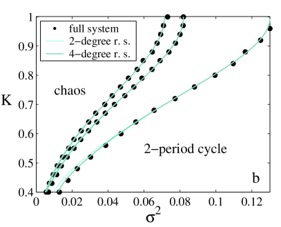
Figure 5: a) The fourth order parameter $\Omega_{4}$ versus the second $\Omega_{2}$ for the population of logistic maps (back dots) and for the reduced system of fourth degree Eq. (17). The continuous line is the invariant manifold which embeds the dynamics of the second and third degree Eqs. (14) and (16) and of the reduced system of zeroth degree Eq. (7) (square). b) First period-doubling bifurcation lines for the full (dots), for reduced system of second degree Eq. and fourth degree Eq. (17). The zeroth degree approximation would give vertical lines corresponding to the bifurcation values for $K=1$.

Finally, we project the macroscopic attractor onto the plane $(\Omega_{2},\Omega_{4})$, as shown in Fig. 5(a). In the reduced system at zeroth degree, the two order parameters coincide with the noise distribution moments and thus identify with the point $(\sigma^{2},m_{4})$. In the reduced systems of both second and third degree, instead, the dynamics of $\Omega_{4}$ is embedded in the invariant line defined by the conservation relation Eq. (15). In the reduced system of fourth degree in $(1-K)$, the fourth order parameter is an independent variable. Figure 5(a) shows that its dynamics is very close to that of the population and displays a similar folded structure.

As the degree of the truncation is increased, one observes a convergence in the dynamics of the lower-order variables. Thus, the reduced system of fourth degree does not visibly improve the agreement of the lowest degree order parameters with the macroscopic variables of the population. As expected, the fourth degree approximation is significantly better only at low coupling values, close to the clustering region. This is clear at weak noise values, when this reduced system provides a better approximation for the macroscopic bifurcations diagram than the lower degree ones (Fig. (5(b)).

The distance between the full system attractor and that of the reduced system of lowest degree can be computed as the mean square distance of $X$ from the parabola defined by Eq. (10)). It scales as $(1-K)^{2}$ for fixed noise intensity in a large region of the parameter space.[12]  This confirms that the approximation to second degree indeed captures the most important deviation of the population dynamics from the reduced system of zeroth degree. Similarly, the distance of the fourth order parameter from the line Eq. (15), valid for the approximations to second and third degree, scales as $(1-K)^{4}$ when the coupling strength is varied.

We conclude that our order parameter expansion describes well the fine structure of the macroscopic attractor. In particular, the fact that we can unveil finer and finer folds by adding higher order parameters suggests that the hierarchy of the folds is well captured by the hierarchy of the reduced system. We now turn our attention to the dynamics occurring on this complex object, trying to quantify the dimensionality of the macroscopic chaos observed and to assess to what extent it is reproduced by our approximations.

4 Lyapunov spectrum of the macroscopic dynamics

In this section, we show that the Lyapunov exponents of the reduced system correspond exactly to the largest macroscopic Lyapunov exponents of the full system.

These largest macroscopic Lyapunov exponents are most easily computed from the dynamics of the full system expressed in terms of the evolution of the probability distribution function (pdf) $\rho_{t}(x)$ of all elements at time $t$. This pdf is governed by the so-called nonlinear Perron-Frobenius operator:[17, 10, 31]

$$\rho_{t+1}(x)=\int{G\left\{F_{t}(y)-x\right\}\,\rho_{t}(y)\,dy}$$ (11)

where $G\{z\}$ is the noise distribution and $F_{t}$ the iterate of the map:

$$F_{t}(y)=\left(1-K\right)\,f(y)+K\int\rho_{t}(z)\,dz.$$

Numerically, this is implemented easily by choosing a sufficiently fine binning of the support of the pdf, which is then represented by a vector. The Lyapunov exponents are computed from this discretized system with the method of Benettin et al.,[32]  following the evolution of a step perturbation of the pdf, according to the formula:

$$\lambda_{i}=\frac{1}{T}\sum_{t=1}^{T}\log(\Delta_{i}^{t}),$$ (12)

where $\Delta_{i}^{t}$ is the ratio between the Euclidean norm of the $i$-th component of a vector basis at time $t-1$ and its corresponding component of the basis at time $t$. This last basis is recomputed at each time step, after a sufficiently long transient, by orthonormalizing the image of the basis of the tangent space at time $t-1$.

We compute the Lyapunov exponents of the reduced system by evaluating explicitly the Jacobian of the system and by computing the iterates of vectors belonging to the tangent space. For the case of the Perron-Frobenius operator, instead, we iterate perturbations of small size along a trajectory. The perturbation size has to be chosen such that the dynamics remains close to the linear regime and a sufficient numerical precision is maintained. The perturbation size appeared not to be a critical parameter, except for the region close to maximal coupling $K=1$.

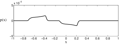
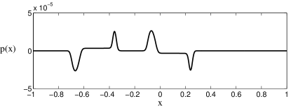
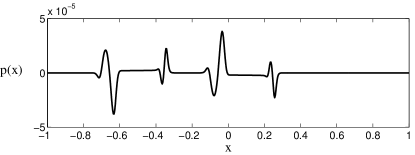
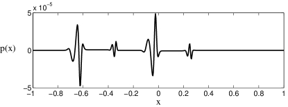
Figure 6: Eigenvectors relative to the four largest Lyapunov exponents for the population of noisy logistic maps ($K=0.5$ and $\sigma^{2}=0.03$).

In this region there are directions converging very fast, so that one time step may be sufficient to greatly flatten the small-scale structures of a distribution, leading to a decrease of numerical precision. This effect appears as a small deviation between the full system and the reduced one for the higher moments when $K$ approaches $1$. In the following, we have checked that our results do not depend on the level of discretization of the support, insuring the extensivity of the spectrum.

In Fig. 6 we show the eigenvectors (in the space of the pdfs) relative to the dominant Lyapunov exponents in a typical case. The increasing steepness of these objects as one goes down the Lyapunov spectrum signals that a reliable determination of many exponents is a computationally demanding task.

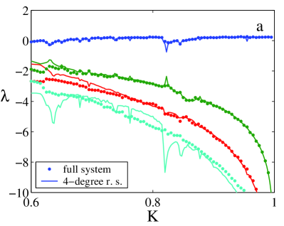
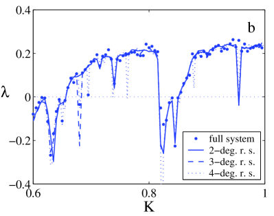
Figure 7: a) Lyapunov exponents of the population (dots) and of the reduced system of fourth degree (solid lines) as a function of the coupling strength, for fixed noise intensity $\sigma^{2}=0.03$. b) Maximal Lyapunov exponent of the population (dots) and of the reduced systems of second (solid line), third (dashed line) and fourth degree (dotted lines) as a function of the coupling strength, for fixed noise intensity $\sigma^{2}=0.03$. The fourth degree truncation provides a slightly better approximation for the lower values of the coupling in the displayed range.

In Fig. 7(a), we show the four largest Lyapunov exponents for the full system and for the reduced system of fourth degree as a function of the coupling strength $K$ and for fixed noise intensity. Clearly, the reduced system captures the main features of the macroscopic dynamics, i.e. the existence of only one positive Lyapunov exponent (magnified in Fig. 7(b)). The quantitative agreement with the population is extremely good for the first two exponents. The discrepancy on the third and fourth exponent, evident for couplings close to the maximal one, are due to a degradation of the numerical accuracy when some directions are too strongly attractive. The quantitative correspondence between the population and the reduced system, especially as far as the third and fourth exponents are concerned, is also lost for too low values of the coupling, where the introduced approximation is likely to be insufficient to take every detail into account.

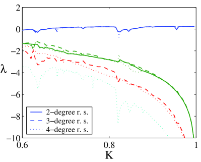
Figure 8: Lyapunov exponents of the reduced system to second (two solid lines), third (three dashed lines) and fourth degree (four dotted lines) as a function of the coupling strength, for fixed noise intensity $\sigma^{2}=0.03$.

In the $K\to 1$ limit the maximum Lyapunov exponent tends to the value which can be derived from the exact scalar map Eq. (6), while all the other directions are all the more attracting as $K$ is close to 1. The truncations of degree greater than zero provide the successive exponents, each approximation level adding one new exponent which is more negative than those retrieved with the truncations to lower degree. This can be seen in Fig. 8, which displays the Lyapunov exponents of the reduced system at different truncation levels.

In view of the obtained quantitative and qualitative agreement with the Lyapunov exponents of the population, we conclude that, in spite of being just one of the possible projections of the population dynamics on a lower dimensional space, the order parameter expansion indeed captures the hierarchical structure of the macroscopic dynamics.

4.1 Dimension of the macroscopic attractor

The computation of the Lyapunov exponents also allows us to address the delicate problem of how the macroscopic attractor dimension depends on the population parameters $K$ and $\sigma$. The question of whether the collective behavior is truly low-dimensional, or instead always infinite-dimensional, has been mainly addressed in the context of weakly-coupled noiseless maps.[18, 24, 7, 33, 34]  Shibata, Chawanya and Kaneko pointed out that, for weak coupling, it is sufficient to add a small amount of noise to reduce drastically the dimensionality of the collective motion, measured as the number of positive Lyapunov exponents of the spectrum of the Perron-Frobenius operator.[10, 31]

Here we approach this question starting from maximal coupling (full synchronization) rather than from zero coupling and compare the attractors of the full and reduced systems on the basis of their Lyapunov or Kaplan-Yorke dimension:

$$D_{L}=j+\frac{\sum_{k=1}^{j}\lambda_{k}}{|\lambda_{j+1}|}$$ (13)

where $j$ is the smallest integer such that, if the Lyapunov exponents $\lambda_{k}$ are listed in descending order, $\sum_{k=1}^{j}\lambda_{k}\geq 0$. The Kaplan-Yorke conjecture, which states that the fractal dimension of a strange attractor is equal to $D_{L}$ [35] appears to hold well for sufficiently nonsingular maps, and has been proved to be an upper estimate of the fractal dimension for a class of maps. [36]  We thus expect to be able to use the Lyapunov dimension as a measure of the dimension of the macroscopic attractor.

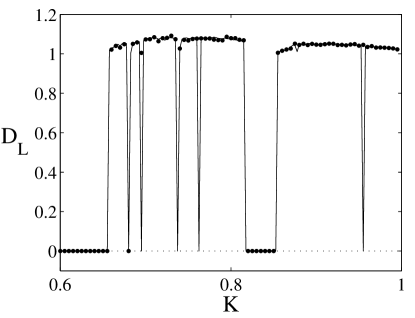
Figure 9: Lyapunov dimension of the macroscopic attractor for the population (dots) and the reduced system to the fourth degree (solid line). The scan corresponds to the bifurcation diagram Fig. 3, for $\sigma^{2}=0.03$. The values of the Lyapunov dimension of the reduced systems of lower degree nearly overlap with those of the fourth degree, and therefore are not displayed.

Although the addition of more and more macroscopic degrees of freedom improves the description of the mean field attractor by revealing smaller scale structures, as we discussed in Section 3, this does not necessarily lead to an increase in the dimension of the macroscopic attractor. Indeed, in the region of interest here, the macroscopic attractor is always characterized by one positive Lyapunov exponent and its increase in dimension is associated to changes of the attractiveness of the transversal modes. If the coupling is sufficiently strong, the dimension of the attractor is less than two and is determined only by the first one of these modes, that associated with the second order parameter.

In Fig. 9, we show that the Lyapunov dimension of the reduced system has the same dependence on the population parameters as that of the population. In particular, this dimension tends to one for $K\to 1$, that is where we have analytically concluded that the macroscopic attractor is strictly one-dimensional. Weakening the coupling, instead, one observes an increase in the attractor dimension, until the system exits the chaotic region through a macroscopic bifurcation, and the Lyapunov dimension drops to zero. Similarly, the intervals within the chaotic region in which the dimension of the macroscopic attractor is zero correspond to the windows of periodic behavior that one can identify in the bifurcation diagram shown in Fig. 3.

5 Discussion

We have studied the macroscopic attractor of large populations of noisy maps. We have shown that, for sufficiently strong coupling, there exists a truncation of the order parameter expansion which is able to reproduce the collective dynamics to any given scale of description. For a fixed coupling, the macroscopic dynamics is effectively described by a sufficiently large number $n$ of order parameters. In this approximation, some of the following order parameters are slaved to the first ones, while all the others can be approximated by the noise distribution moments within the error of a macroscopic description. The hierarchy of reduced systems obtained in such a manner reflects the fractal structure of the mean field attractor, that can be described on a finer and finer scale as the degree of approximation is increased. In spite of its complex structure embedded into an infinite-dimensional phase, however, the macroscopic attractor has a finite Lyapunov dimension, which is the same as that of the reduced systems.

Some further questions that can be addressed by means of the reduced systems are whether the macroscopic attractor attains its maximum Lyapunov dimension for fixed noise intensity and how this maximum value changes with $\sigma^{2}$. In particular, it would be interesting to determine whether this maximal dimension converges to a finite value in the limit of weak noise for any coupling strength.

From the order parameter expansion, it is clear that the moments of the noise distribution constitute the most relevant terms in the evolution of the order parameter of corresponding degree. In the limit of maximal coupling, thus, the order parameter of $q$-th degree scales “normally”, that is proportionally to $\sigma^{q}$. For coupling less than maximal, these iterates are perturbed by the macroscopic dynamics, so that one can identify deviations from the normal scaling associated with the bifurcations of the mean field attractor. It is in principle conceivable that such bifurcations give rise to the “anomalous scaling” observed for intermediate coupling strengths, close to the point where the synchronous regime breaks down for a population of noiseless maps. Another possibility is that for intermediate couplings the effective dimensionality of the mean field dynamics diverges, so that no finite truncation is able to capture the scaling of the order parameters with the noise intensity. In order to answer this question, we are now exploring the region of low coupling/weak noise close to the turbulent regime, where the attractors for the low-dimensional reduced systems presented in this paper become unstable.

Appendix A Reduced systems up to fourth degree for logistic maps

We explicitly derive the reduced systems for the case where individual maps have the quadratic form Eq. (3). The explicit form of $A_{q}$ and $\Gamma_{i}$ are obtained following the procedure illustrated in the derivation of Eq. (5) [15]: first, we write the equations for the first $2n$ moments and then we eliminate $n$ ’slaved’ degrees of freedom by noticing that certain linear combinations of the order parameters are invariant.

As we have seen in the paragraph 2.2, Eq. (5) to the zeroth degree yields Eq. (7).

The second degree reduces system reads:

$$\begin{cases}X\mapsto&1-a\,X^{2}-a\>\Omega_{2}\\ \Omega_{2}\mapsto&\sigma^{2}+(1-K)^{2}\>a^{2}\left[m_{4}-6\sigma^{4}+(4X^{2}-\Omega_{2}+6\>\sigma^{2})\>\Omega_{2}\right]\end{cases}$$ (14)

and the two conservation relations are valid:

$$\Omega_{3}= m_{3}$$

$$\Omega_{4}= m_{4}+6\,\sigma^{2}\left(\Omega_{2}-\sigma^{2}\right).$$ (15)

The third degree reduced system is the three-dimensional macroscopic map:

$$\begin{cases}X\mapsto&1-a\,X^{2}-a\>\Omega_{2}\\ \Omega_{2}\mapsto&\sigma^{2}+(1-K)^{2}\>a^{2}\>\Sigma_{2}\\ \Omega_{3}\mapsto&-(1-K)^{3}\>a^{3}\>\Sigma_{3}\end{cases}$$ (16)

where:

$$\Sigma_{2}= m_{4}-6\,\sigma^{4}+6\,\sigma^{2}\,\Omega_{2}-\Omega_{2}^{2}+4\,X^{2}\,\Omega_{2}-4\,X\,\Omega_{3}$$

$$\Sigma_{3}= m_{6}-15\,m_{4}\,\sigma^{2}+\left(12\,m_{4}-72\,\sigma^{4}\right)\,X^{2}+\left(12\,m_{4}+18\,\sigma^{4}\right)\,\Omega_{2}+72\,\sigma^{2}\,X^{2}\,\Omega_{2}$$

$$-18\,\sigma^{2}\,\Omega_{2}^{2}-12\,X^{2}\,\Omega_{2}^{2}+2\,\Omega_{2}^{3}-12\,X\,\Omega_{2}\,\Omega_{3}+8\,X^{3}\,\Omega_{3}.$$

The following three order parameters are slaved to the first three macroscopic variables and they obey the relations:

$$\Omega_{4}= m_{4}+6\,\sigma^{2}\left(\Omega_{2}-\sigma^{2}\right)$$

$$\Omega_{5}= 10\,\sigma^{2}\,\Omega_{3}$$

$$\Omega_{6}= m_{6}+15\,m_{4}\left(\Omega_{2}-\sigma^{2}\right),$$

while $\Omega_{q}=m_{q}$ holds for $q>6$.

The truncation of the order parameter expansion to the fourth degree is the four-dimensional macroscopic map:

$$\begin{cases}X\mapsto&1-a\,X^{2}-a\>\Omega_{2}\\ \Omega_{2}\mapsto&\sigma^{2}+(1-K)^{2}\>a^{2}\>\Sigma_{2}\\ \Omega_{3}\mapsto&(1-K)^{3}\>a^{3}\>\Sigma_{3}\\ \Omega_{4}\mapsto&m_{4}+6\>\sigma^{2}\>(1-K)^{2}\>a^{2}\Sigma_{2}+(1-K)^{4}\>a^{4}\>\Sigma_{4}\end{cases}$$ (17)

where:

$$\Sigma_{2}= \Omega_{4}-\Omega_{2}^{2}+4\,X^{2}\,\Omega_{2}+4\,X\,\Omega_{3}$$

$$\Sigma_{3}= \Omega_{6}+6\,X\,\left(\Omega_{5}-2\,\Omega_{2}\,\Omega_{3}\right)-3\,\Omega_{2}\,\Omega_{4}+8\,X^{3}\,\Omega_{3}-12\,X^{2}\,\left(\Omega_{2}^{2}-\Omega^{4}\right)+2\Omega_{2}^{3}$$

$$\Sigma_{4}= \Omega_{8}+8\,X\,\left(3\,\Omega_{2}^{2}\,\Omega_{3}-2\,\Omega_{2}\,\Omega_{5}+\Omega_{7}\right)+24\,X^{2}\left(\Omega_{2}^{3}-2\,\Omega_{2}\,\Omega_{4}+\Omega_{6}\right)-4\Omega_{2}\,\Omega_{6}$$

$$-32X^{3}\left(\Omega_{2}\,\Omega_{3}-\Omega_{5}\right)+6\Omega_{2}^{2}\,\Omega_{4}+16X^{4}\,\Omega_{4}-3\Omega_{2}^{4}.$$

The successive order parameters depend linearly on the first ones according to the relations:

$$\Omega_{5}= 10\,\sigma^{2}\,\Omega_{3}$$

$$\Omega_{6}= m_{6}+\left(m_{4}-6\,\sigma^{4}\right)\left(\Omega_{2}-\sigma^{2}\right)+\sigma^{2}\left(\Omega_{4}-m_{4}\right)$$

$$\Omega_{7}= 35\,m_{4}\,\Omega_{3}$$

$$\Omega_{8}= m_{8}+28\,\left(m_{6}-15\,m_{4}\,\sigma^{2}\right)\left(\Omega_{2}-\sigma^{2}\right)+70\,m_{4}\left(\Omega_{4}-m_{4}\right)$$

and the remaining order parameters are equal to the noise distribution moments.

References

- [1] T. Bohr, G. Grinstein, Yu He, and C. Jayaprakash. Coherence, chaos, and broken symmetry in classical, many-body dynamical systems. Phys. Rev. Lett., 58:2155, 1987.
- [2] K. Kaneko. Clustering, coding, switching, hierarchical ordering, and control in a network of chaotic elements. Physica D, 41:137, 1990.
- [3] P. C. Matthews, R. E. Mirollo, and S. H. Strogatz. Dynamics of a large system of coupled nonlinear oscillators. Physica D, 52:293, 1991.
- [4] N. Nakagawa and Y. Kuramoto. Collective chaos in a population of globally coupled oscillators. Progress of Theoretical Physics, 89:313–323, 1993.
- [5] N. Nakagawa and Y. Kuramoto. From collective oscillations to collective chaos in a globally coupled oscillator system. Physica D, 75:74–80, 1994.
- [6] N. Nakagawa and Y. Kuramoto. Anomalous Lyapunov spectrum in globally coupled oscillators. Physica D, 80:307–316, 1995.
- [7] T. Chawanya and S. Morita. On the bifurcation structure of the mean-field fluctuations in the globally coupled tent map systems. Physica D, 116:44, 1998.
- [8] T. Shibata and K. Kaneko. Collective chaos. Phys. Rev. Lett., 81:4116, 1998.
- [9] M. Cencini, M. Falcioni, D. Vergni, and A. Vulpiani. Macroscopic chaos in globally coupled maps. Physica D, 130:58, 1999.
- [10] T. Shibata, T. Chawanya, and K. Kaneko. Noiseless collective motion out of noisy chaos. Phys. Rev. Lett., 82:4424, 1999.
- [11] J. Teramae and Y. Kuramoto. Strong desynchronizing effects of weak noise in globally coupled systems. Phys. Rev. E, 63:036210, 2001.
- [12] S. De Monte, F. d’Ovidio, H. Chaté, and E. Mosekilde. Noise-induced macroscopic bifurcations in globally coupled chaotic units. Phys. Rev. Lett., 92:254101, 2004.
- [13] S. De Monte and F. d’Ovidio. Dynamics of order parameters for globally coupled oscillators. Europhys. Lett., 58:21, 2002.
- [14] S. De Monte, F. d’Ovidio, and E. Mosekilde. Coherent regimes of globally coupled dynamical systems. Phys. Rev. Lett., 90:054102, 2003.
- [15] S. De Monte, F. d’Ovidio, H. Chaté, and E. Mosekilde. Effects of microscopic disorder on the collective dynamics of globally coupled maps. Physica D, 205:25–40, 2005.
- [16] K. Kaneko. Mean Field Fluctuation in Network of Chaotic Elements Physica D, 55:368, 1992.
- [17] A. Pikovsky and J. Kurths. Do globally coupled maps really violate the law of large numbers? Phys. Rev. Lett., 72:1644, 1994.
- [18] K. Kaneko. Remarks on the mean field dynamics of networks of chaotic elements. Physica D, 86:158, 1995.
- [19] S. Morita. Scaling law for the lyapunov spectra in globally coupled tent maps. Physical Review E, 58:4401–4412, 1998.
- [20] K. Kaneko. Globally coupled chaos violates the law of large numbers but not the central-limit theorem. Phys. Rev. Lett., 65:1391-1394, 1990.
- [21] H. Chaté and P. Manneville. Evidence of collective behaviour in cellular automata. Europhys. Lett., 14:409, 1991.
- [22] A. Maritan and J.R. Banavar. Chaos, noise, and synchronization. Phys. Rev. Lett., 72:1451, 1994.
- [23] A. Pikovsky. Comment on “Chaos, noise and synchronization”. Phys. Rev. Lett., 73:2931, 1994.
- [24] N. Nakagawa and T. S. Komatsu. Collective motion occurs inevitably in a class of populations of globally coupled chaotic elements. Phys. Rev. E, 57:1570, 1998.
- [25] S. C. Manrubia and A. S. Mikhailov. Very long transients in globally coupled maps. Europhys. Lett., 50:580, 2000.
- [26] T. Shimada and S. Tsukada. Periodicity manifestations in the non-locally coupled maps. Physica D, 168-169:126, 2000.
- [27] O. Popovych, Y. Maistrenko, and E. Mosekilde. Loss of coherence in a system of globally coupled maps. Phys. Rev. E, 64:026205, 2001.
- [28] O. Popovych, Y. Maistrenko, and E. Mosekilde. Role of asymmetric clusters in desynchronization of coherent motion. Physics Letters A, 302:171, 2002.
- [29] H. Hong and M.Y. Choi. Phase synchronization and noise-induced resonance in systems of coupled oscillators. Phys. Rev. E, 62:6462, 2000.
- [30] S. De Monte et al. in preparation.
- [31] T. Shibata. Collective chaos, 1999. PhD. thesis, University of Tokyo.
- [32] G. Benettin, L. Galgani, A. Giorgilli, and J-M. Strelcyn. Lyapunov characteristic exponents for smooth dynamical systems and for hamiltonian systems: a method for computing all of them. part 1: Theory. Meccanica, page 9, 1980.
- [33] N. Nakagawa and T. S. Komatsu. Confined chaotic behaviour in collective motion for populations of globally coupled chaotic elements. Phys. Rev. E, 59:1675, 1999.
- [34] D. Topaj, W.Kye, and A. Pikovsky. Transition to coherence in populations of coupled chaotic oscillators: a linear response approach. Phys. Rev. Lett., 87:074101, 2001.
- [35] E. Ott. Chaos in dynamical systems. Cambridge University Press, 1993.
- [36] P. Grassberger and I. Procaccia. Measuring the strangeness of strange attractors. Physica D, 9:189, 1983.