Dynamics of coupled Josephson junctions under the influence of applied fields

Abstract

We investigate the effect of the phase difference of applied fields on the dynamics of mutually coupled Josephson junction. The system desynchronizes for any value of applied phase difference and the dynamics even changes from chaotic to periodic motion for some values of applied phase difference. We report that by keeping the value of phase difference as $\pi$, the system continues to be in periodic motion for a wide range of system parameter values which might be of great practical applications.

and

1 Introduction

The study of the dynamics of Josephson junction (JJ) is of fundamental and experimental interest. The interaction of Josephson junctions with external fields have played an important role in the development of Josephson physics and its chaotic dynamics [1, 2, 3, 4]. The existence of chaos in rf-biased Josephson junction has been verified through theory, numerical simulation and experiments [5]. The rf-biased junction is of practical importance because of its application as voltage standards, a situation where chaotic behavior is least desired [6]. Control of chaos is an active area of research [7] because of the many undesirable effects chaos brings in mechanical systems and other devices. It was shown to be possible to control chaos both theoretically and experimentally using different methods such as giving a feed back [8], application of a weak periodic force [9] etc. The problem of controlling spatiotemporal chaotic pattern induced by an applied rf signal in a Josephson junction has earlier been discussed [10]. By controlling chaos in rf-biased Josephson junctions it was shown that even in the presence of thermal noise they can be used as voltage standards [11]. Suppression of temporal and spatio-temporal chaos allows complex systems to be operated in highly nonlinear regimes. This is a desirable feature in many physical systems. By applying a small time-dependent modulation to a parameter, a chaotic system can be stabilzed. However in practical applications this method requires that the characteristic times of the system is not too short compared with the times of the feed back system. In the case of JJ oscillators the characteristic times of the dynamics response are of the orders of few picoseconds which is too short for any electronic feedback control system.

Since it was shown that chaotic systems could be synchronized by linking them with common signal [12] many works have been done in this direction because of its application in secure communication [13]. Synchronization in Josephson junction has been an interesting area of research [14, 15, 16]. The role of phase difference of applied sinusoidal fields in desynchronizing and suppressing chaos in duffing oscillators has been studied [17, 18]. In the present work, we consider the effect of phase difference of the applied rf-fields on mutually coupled Josephson junctions. We discuss the equation of coupled JJ in section II and arrive at the dimensionless first order form of the equation of motion of the system. In section III the parameter range in which the system is synchronized is found and the effect of phase difference of the applied rf fields on synchronization is found. We analyze the dynamics of the Josephson junction after applying the phase difference. Then by fixing a particular phase value where the system becomes periodic we discuss the effect of other parameters on the junction. In section IV the results are discussed and the applications are mentioned.

2 THEORY

Josephson junction can be represented by a resistively and capacitively shunted junction (RCSJ) model and the dynamics of the system can be explored by writing the equation of motion [19]. The equation of a single Josephson junction by this model can be written by solving Kirchoff’s law as

$$\frac{\hbar C}{2e}\frac{d^{2}\phi}{dt^{2}}+\frac{\hbar}{2eR}\frac{d\phi}{dt}+i_{c}\sin\phi=i_{dc}+i_{0}\cos(\omega t),$$ (1)

where $\phi$ is the phase difference of the wave function across the junction, $i_{0}\cos(\omega t)$ is the driving rf - field and $i_{dc}$ is the dc bias. The junction is characterized by a critical current $i_{c}$, capacitance $C$ and normal resistance $R$. The coupled JJ considered here consists of a pair of such junctions wired in parallel with a linking resistor $R_{s}$ [15]. Such a system can be schematically given as in Fig(1) and the dynamical equations can be written as

Figure 1: Schematic representation of a coupled Josephson junction connected in parallel with a linking resistor $R_{s}$. 1 and 2 represents the applied fields.

$$\frac{\hbar C_{1}}{2e}\frac{d^{2}\phi_{1}}{dt^{\prime 2}}+\frac{\hbar}{2eR_{1}}\frac{d\phi_{1}}{dt^{\prime}}+i_{c1}\sin\phi_{1}=i_{dc}^{\prime}+i_{0}^{\prime}\cos(\omega t^{\prime})-i_{s}$$ (2)

$$\frac{\hbar C_{2}}{2e}\frac{d^{2}\phi_{2}}{dt^{\prime 2}}+\frac{\hbar}{2eR_{2}}\frac{d\phi_{2}}{dt^{\prime}}+i_{c2}\sin\phi_{2}=i_{dc}^{\prime}+i_{0}^{\prime}\cos(\omega t^{\prime}+\theta)+i_{s},$$ (3)

where $i_{s}$ is the current flowing through the coupling resistor and is given as

$$i_{s}=\frac{\hbar}{2eR_{s}}\left[\frac{d\phi_{1}}{dt^{\prime}}-\frac{d\phi_{2}}{dt^{\prime}}\right].$$ (4)

In order to express Eqs.(2) and (3) in dimensionless, normalized form we introduce the junction plasma frequencies $\omega_{J1}$ and $\omega_{J2}$ which are given by $\omega_{J1}=\left(2ei_{c1}/\hbar C_{1}\right)^{\frac{1}{2}}$ and $\omega_{J2}=\left(2ei_{c2}/\hbar C_{2}\right)^{\frac{1}{2}}$ and also normalized time scale as $t=\omega_{J1}t^{\prime}$. The dimensionless damping parameter is defined as

$$\beta=\frac{1}{R_{1}}\sqrt{\frac{\hbar}{2ei_{c1}C_{1}}}.$$

The dc bias current $i_{dc}^{\prime}$ and the rf amplitude $i_{0}^{\prime}$ are normalized to the critical current $i_{c1}$. We also normalize the actual frequency $\omega$ to $\Omega=\omega/\omega_{J1}$ and $\alpha_{s}=\left(R_{1}/R_{s}\right)\beta$.

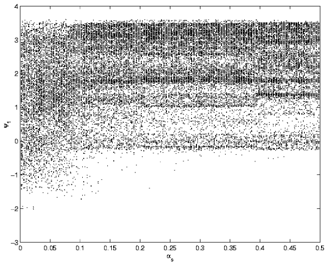
Figure 2: Maxima of the normalized voltage plotted against coupling strength $\alpha_{s}$ for $\theta=0$, $\beta=0.15$, $i_{0}=0.7$ and $\omega=0.6$.

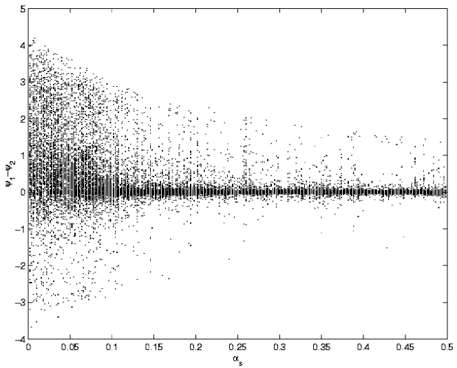
Figure 3: Maxima of the difference in voltage against coupling strength $\alpha_{s}$. $\theta=0$, $\beta=0.15$, $i_{0}=0.7$ and $\omega=0.6$.

For identical Josephson junctions, we can write Eqs.(2) and (3) as

$$\ddot{\phi_{1}}+\beta\dot{\phi_{1}}+\sin\phi_{1} = i_{dc}+i_{0}\cos(\Omega t)-\alpha_{s}\left[\dot{\phi_{1}}-\dot{\phi_{2}}\right],$$

$$\ddot{\phi_{2}}+\beta\dot{\phi_{2}}+\sin\phi_{2} = i_{dc}+i_{0}\cos(\Omega t+\theta)-\alpha_{s}\left[\dot{\phi_{2}}-\dot{\phi_{1}}\right].$$ (5)

It can be seen that the coupling arises as a natural consequence of the exchange of current through the resistor $R_{s}$ and it depends on the differential voltage ($\psi_{1}-\psi_{2}$). For Josephson junction devices, phase derivatives are of central importance because they are proportional to junction voltages. In order to study the system numerically we write the above equations in the first order differential form as

$$\dot{\phi_{1}} = \psi_{1},$$

$$\dot{\psi_{1}} = -\beta\psi_{1}-\sin\phi_{1}+i_{dc}+i_{0}\cos(\Omega t)-\alpha_{s}\left[\psi_{1}-\psi_{2}\right],$$

$$\dot{\phi_{2}} = \psi_{2},$$ (6)

$$\dot{\psi_{2}} = -\beta\psi_{2}-\sin\phi_{2}+i_{dc}+i_{0}\cos[(\Omega t)+\theta]-\alpha_{s}\left[\psi_{2}-\psi_{1}\right].$$

Eq. (2) is studied using fourth order Runge-Kutta method and the maxima of normalized voltage values are plotted to study the dynamics. It was observed that the system exhibits chaotic behavior for $\beta=0.15$, $i_{0}=0.7$, $i_{dc}=0.3$ and $\Omega=0.6$ as seen in Fig. 2. From Fig. 3 we can see that the difference in voltage becomes smaller as the coupling strength is increased.

3 The effect of Phase Difference

The effect of phase difference of the applied sinusoidal driving field on coupled periodically driven duffing oscillator has been studied [18] and it was observed that the system desynchronizes by the application of a phase difference. To study how the phase difference of the applied fields acts on JJ system we write $S_{\phi}=\phi_{1}-\phi_{2}$ and $S_{\psi}=\psi_{1}-\psi_{2}$ and from Eq. (2) we get

$$\dot{S_{\phi}} = S_{\psi},$$ (7)

$$\dot{S_{\psi}} = -\beta S_{\psi}-\sin\phi_{1}+\sin\phi_{2}-2\alpha_{s}S_{\psi}+2i_{0}\sin\left(\Omega t+\frac{\theta}{2}\right)\sin\left(\frac{\theta}{2}\right).$$

When $\theta=0$ the term $2i_{0}\sin\left(\Omega t+\theta/2\right)\sin\left(\theta/2\right)$ vanishes. We choose the values of $\alpha_{s}$ such that the difference in voltage is negligible. ie., $\psi_{1}\approx\psi_{2}$. Now both $\dot{S_{\phi}}$ and $\dot{S_{\psi}}$ go to zero. From Fig. 3 we select our value of $\alpha_{s}$ as $0.45$ which almost satisfies this condition. From Eq. 7 we can see that even for small values of phase differences $\dot{S_{\psi}}\neq 0$ and the system desynchronizes. Figs. 4(a) and 4(c) show that the system is synchronized and Figs. 4(b) and 4(d) show that the system is desynchronized by an applied phase difference of $\theta=0.1\pi$. The level of mismatch of chaos synchronization can be given quantitatively by taking the similarity function $S(\tau)$ as a time averaged difference between the variables $\psi_{1}$ and $\psi_{1}$ taken with time shift $\tau$ [20]

$$S^{2}(\tau)=\frac{\langle\left[\psi_{1}(t+\tau)-\psi_{2}(t)\right]^{2}\rangle}{\left[\langle\psi_{1}^{2}(t)\rangle\right]\left[\langle\psi_{2}^{2}(t)\rangle\right]^{1/2}}.$$ (8)

We plot $S(\tau)$ against $\tau$ for different values of phase difference $\theta$ as shown in Fig. 5. It is observed that for $\theta=0$, the system is in complete synchronization. For a finite value of phase difference we observe that a minimum of $S(\tau_{0})$ appears which indicates the existence of a certain phase difference between the interacting systems. $S(\tau_{0})$ is finite in these cases which means that in this regime the amplitudes are uncorrelated.

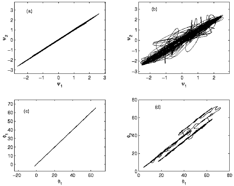
Figure 4: a and c show the system is synchronized for $\theta=0$, $\beta=0.15$, $i_{0}=0.7$, $i_{dc}=0.3$, $\alpha_{s}=0.45$ and $\omega=0.6$. b and d show the system desynchronized for a phase difference of $\theta=0.1\pi$

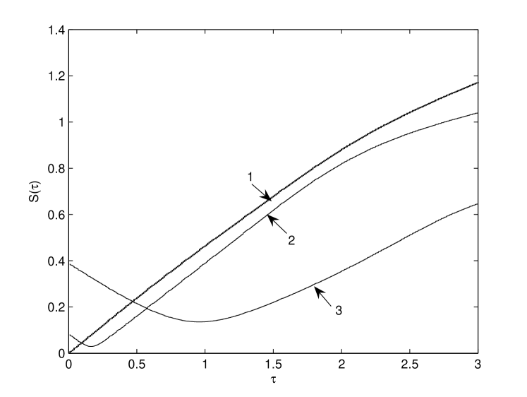
Figure 5: Similarity function $S(\tau)$ versus $\tau$ for different values of phase difference $\theta$. Curve 1 is with phase difference $\theta=0$, 2 for $\theta=0.1\pi$ and 3 for $\theta=0.5\pi$.

Now we vary the values of $\theta$ from $0$ to $2\pi$ and plot the maxima of the difference in voltage against the phase. It can be observed from Fig. 6 that the system passes from chaotic to periodic motion for some values of $\theta$. In the synchronization manifold, ie., when $\phi_{1}=\phi_{2}$ and $\psi_{1}=\psi_{2}$ we can write $P_{\phi}=\left[\phi_{1}+\phi_{2}\right]/2$ and $P_{\psi}=\left[\psi_{1}+\psi_{2}\right]/2$ and from Eq. (2) we get

$$\dot{P_{\phi}} = P_{\psi},$$ (9)

$$\dot{P_{\psi}} = -\beta P_{\psi}-\sin(P_{\phi})+idc+i_{0}\cos\left(\frac{\theta}{2}\right)\cos\left(\Omega t+\frac{\theta}{2}\right).$$

Eq. (9) is equivalent to Eq. (1) and we can see that $i_{0}$ is replaced by $i_{0}\cos\left(\theta/2\right)$ and the phase of the driving field leads by $\theta/2$ as a result of coupling. This might correspond to a parameter space where the system is periodic which explains the change in system dynamics.

The variation of the voltage of one junction with the applied phase difference is shown in Fig. 7. From the inset of Fig. 6 it can be seen that the system exhibits periodic window in the region where $\theta=0.34\pi-0.4\pi$. However in this region even a slight change in system parameter values would bring the system back to chaotic regime. For a phase difference of $\theta=0.95\pi-1.5\pi$ the system exhibits periodic motion and the corresponding periodic difference in voltage and voltage plotted against time is shown in Figs. 8(c) and 8(d). Figs. 8(a) and 8(b) shows difference in voltage and voltage against time for a phase difference of $\theta=0$.

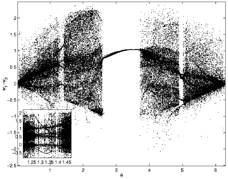
Figure 6: Maxima of the difference in voltage is plotted against phase difference applied, $\theta=0-2\pi$. $\alpha_{s}=0.45$, $i_{dc}=0.3$, $\beta=0.15$, $i_{0}=0.7$ and $\omega=0.6$.

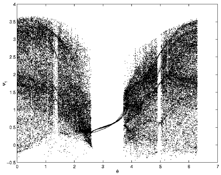
Figure 7: Voltage corresponding to a single junction is plotted for phase values $\theta=0-2\pi$ with $\alpha_{s}=0.45$, $i_{dc}=0.3$, , $\beta=0.15$, $i_{0}=0.7$ and $\omega=0.6$.

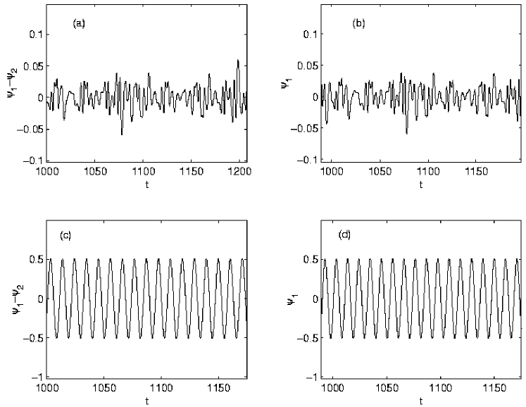
Figure 8: (a) shows the differential voltage plotted against time and (b) is the voltage of one junction with $\theta=0$. It is observed that the variation is chaotic and the maximum difference in voltage is $0.05$. In (c) and (d) shows the corresponding voltages with an applied phase difference of $\pi$. Other parameter values are $\alpha_{s}=0.45$, $\beta=0.15$, $i_{0}=0.7$ and $\omega=0.6$.

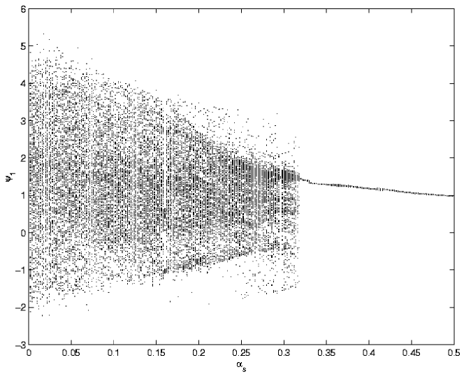
Figure 9: Maxima of the normalized voltage against coupling strength $\alpha_{s}$. $\theta=\pi$, $\beta=0.15$, $i_{dc}=0.3$, $i_{0}=0.7$ and $\omega=0.6$.

Fixing the phase difference between the driving fields as $\pi$, the change in the response of the system to other parameter variations are studied. From Fig. 2 we can see that the system is in chaotic motion even for large values of coupling strength. However by the application of a phase difference of $\pi$ we observe that the system exhibits periodic motion from a coupling strength $0.32$ onwards as can be seen from Fig. 9.

Now we fix the value of $\alpha$ as $0.45$ and the amplitude of the driving rf field is changed from $0$ to $1$. Without an applied phase difference we can see from Fig. 10 that the system exhibits chaotic motion from a value of $0.43$ onwards with some periodic windows in between. However on the application of a phase difference the system stays in periodic state for a wide range of amplitude values which were chaotic earlier. Fig. 11 shows the response of the system when the amplitude of the driving field is changed from $0$ to $1$ with an applied phase difference of $\pi$.

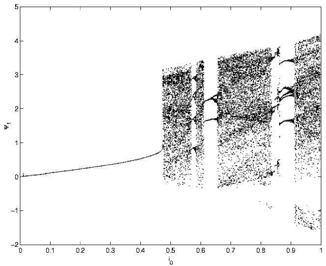
Figure 10: Maxima of the normalized voltage against amplitude of applied field $i_{0}$ with $\theta=0$. The other parameter values are $\alpha_{s}=0.45$, $i_{dc}=0.3$, $\beta=0.15$ and $\omega=0.6$.

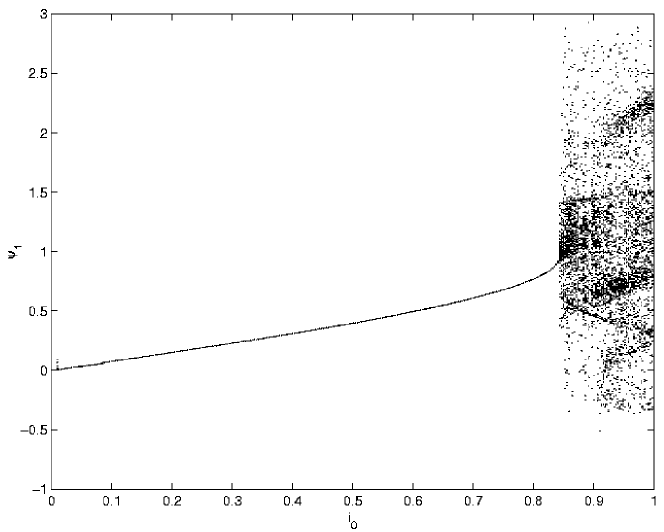
Figure 11: Maxima of the normalized voltage is plotted against the amplitude of applied field. It can be seen that the system is in periodic motion for a wide range of amplitude values. $\theta=\pi$, $\alpha_{s}=0.45$, $i_{dc}=0.3$, $\beta=0.15$ and $\omega=0.6$.

The effect of phase on the applied dc bias on the system is also studied. For this all other parameter values were fixed and $i_{dc}$ value is changed from $0$ to $0.4$. Here also we observe that the system continues to be in periodic motion for a large range of $i_{dc}$ values. The comparison can be obtained from Fig. 12 and Fig. 13. Thus we show that the system exhibits periodic motion for a wide range of parameter values for an applied phase difference between the driving fields. This might be of great practical importance when we consider Josephson junction devices like voltage standards.

An important point to be noted is that the parameter values at which we apply phase difference is to be chosen carefully. If the values we choose is in a region where the difference in voltage ($\psi_{1}-\psi_{2}$) is large, then by just applying a phase difference we may not be able to control chaos.

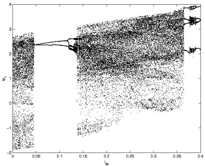
Figure 12: Maxima of the normalized voltage against the $i_{dc}$. $\theta=0$, $\alpha_{s}=0.45$, $\beta=0.15$, $i_{0}=0.7$ and $\omega=0.6$.

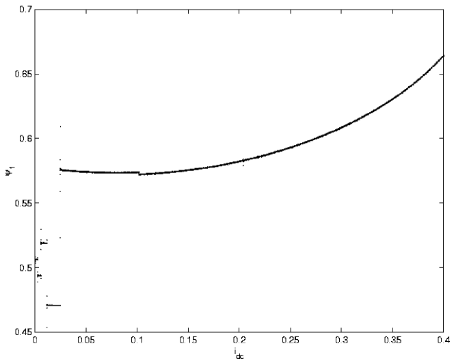
Figure 13: Maxima of the normalized voltage against the $i_{dc}$ . $\theta=\pi$, $\alpha_{s}=0.45$, $\beta=0.15$, $i_{0}=0.7$ and $\omega=0.6$.

4 Conclusion

In this work we find that by applying a phase difference in the driving fields we can control chaos in Josephson junction. We also observe that for this type of control we have to choose the junction parameter values where the difference in voltages between the two junctions is negligible. We report that in a region where the difference in voltages between the two junction is not negligible chaos cannot be controlled by applying a phase difference in the driving fields. For the parameter region we choose the system was in periodic motion for a phase difference of $\theta=0.95\pi-1.5\pi$. Now we fix the phase difference as $\pi$ and vary other parameters such as dc bias, amplitude of applied field and coupling strength. It is found that even for large variation of these parameters, the system continues to be in periodic motion. So this might be of great practical importance as phase difference can be easily applied to the rf-field in an experimental set up. Thus it offers an easier way to control chaos and thus will provide an enhanced capability to design superconducting circuits in such a way as to maximize the advantages of non linearity while minimizing the possibility of instabilities.

References

- [1] N. Grønbech-Jensen, P.S.Lomdahl and M.R.Samuelsen, Phys. Rev. B 43 (1991) 12799.
- [2] D.C.Cronemeyer, C.C.Chi,A.Davidson and N.F.Pedersen, Phys. Rev. B 31 (1985) 2667.
- [3] Wenhua Hai, Yi Xiao, Guishu Chong, Qiongtao Xie Phys. Lett. A 295 (2002) 220.
- [4] W.J.Yeh, O.G.Symko and D.J.Zheng, Phys. Rev. B 42 (1990) 4080.
- [5] R.L.Kautz and J.C.Macfarlane, Phys. Rev. A 33 (1986) 498 and references therein.
- [6] R.L.Kautz and R.Monaco, J. Appl. Phys 57 (1985) 875.
- [7] T. Kapitaniak, Controlling Chaos, Academic press, San Diego, 1996.
- [8] J.Singer, Y.-Z.Wang and Haim.H.Bau, Phys. Rev. Lett. 66 (1991) 1123.
- [9] Y.Braiman, I.Goldhirsch, Phys. Rev. Lett. 66 (1991) 2545.
- [10] O. H. Olsen and M. R. Samuelsen, Phys. Lett. A 266 (2000) 123.
- [11] E. Abraham, I. L. Atkin and A. Wilson, IEEE Trans.Appl. Supercond. 9 (1999) 4166.
- [12] L. M. Pecora and T. L. Carroll, Phys. Rev. Lett. 64 (1990) 821.
- [13] C.-M.Kim, S. Rim, and W.-H. Kye, Phys. Rev. Lett. 88 (2002) 014103.
- [14] A. N. Grib, P. Seidel, and J. Scherbel Phys. Rev. B 65 (2002) 094508.
- [15] J.A.Blackburn, G.L.Baker and H.J.T.Smith, Phys. Rev. B 62 (2000) 5931.
- [16] A. Uçar, K. E. Lonngren and Er-Wei Bai, Chaos Soliton and Fractals (in Press)
- [17] Zhilin Qu, Gang Hu, Guojain Yang and Guangrong Qin, Phys. Rev. Lett. 74 (1995) 1736.
- [18] H.W.Yin, J.H.Dai and H.J. Zhang, Phys. Rev. E 58 (1998) 5683.
- [19] A. Barone and G. Paterno, Physics and Applications of Josephson effect, Wiley, New York, 1982.
- [20] M. G. Rosenblum, A. S. Pikovsky, and J. Kurths, Phys.Rev.Lett. 78 (1997) 4193.