The Role of Redundancy in the Robustness of Random Boolean Networks

Abstract

Evolution depends on the possibility of successfully exploring fitness landscapes via mutation and recombination. With these search procedures, exploration is difficult in “rugged” fitness landscapes, where small mutations can drastically change functionalities in an organism. Random Boolean networks (RBNs), being general models, can be used to explore theories of how evolution can take place in rugged landscapes; or even change the landscapes.

In this paper, we study the effect that redundant nodes have on the robustness of RBNs. Using computer simulations, we have found that the addition of redundant nodes to RBNs increases their robustness. We conjecture that redundancy is a way of “smoothening” fitness landscapes. Therefore, redundancy can facilitate evolutionary searches. However, too much redundancy could reduce the rate of adaptation of an evolutionary process. Our results also provide supporting evidence in favour of Kauffman’s conjecture [Kauffman, 2000, p.195].

Introduction

A system is robust if it continues to function in the face of perturbations [Wagner, 2005a]. This makes robustness a desireable property in any system surrounded by a complex environment. Living systems fall into this category. Systems able to cope with perturbations will survive and reproduce. Moreover, robustness plays a key role in evolvability: it allows the gradual exploration of new solutions while maintaining functionality. A small change in a fragile system would destroy it. This is not favoured if the exploration method consists of random mutations.

There are several mechanisms that help a system to be robust [von Neumann, 1956], such as modularity [Simon, 1996, Watson and Pollack, 2005], degeneracy [Fernández and Solé, 2004], distributed robustness [Wagner, 2004], and redundancy. Here, we focus on this last one. It consists on having more than one copy of an element type. If one fails or changes its function, another can still perform as expected. Redundancy is widespread in genomes of higher organisms [Nowak et al., 1997]. A clear example is seen with diploidy, where each cell has two complete sets of genes. This has several advantages for evolvability, e.g. it provides robustness to recessive detrimental mutations of one gene of a pair. There is also substantial evidence for the hypothesis that growth in genetic regulatory networks occurs primarily via the duplication of genes and subsequent mutations of one or both members of the duplicate pair [Foster et al., 2005, Lewin, 2000]. Thus, it would be desireable to obtain a better understanding of its mechanisms. To achieve this, we used random Boolean networks (RBNs) [Kauffman, 1969, Kauffman, 1993, Wuensche, 1998, Aldana-González et al., 2003, Gershenson, 2004], a very popular model of genetic regulatory networks.

Our present work was initially motivated by Kauffman’s conjecture [Kauffman, 2000, p. 195]. This states that 1-bit mutations to a minimal program will change drastically the output of the program, making it indistinguishable from noise. The conjecture points to the necessity of having some redundancy to allow smooth transitions as a program changes in an evolutionary search.

However, it is not obvious to obtain a minimal program in a standard programming language such as C or Java. Still, we can consider cellular automata (CA) [von Neumann, 1966] or RBNs as programs. It has been shown that certain CA can perform universal computations [Gardner, 1983, Cook, 2004]. Since RBNs are a well studied generalization of CA [Gershenson, 2002], they seem suitable candidates for studying the effect of redundancy in their robustness. We can measure the redundancy of a RBN, make 1-bit mutations to the networks, and then measure their robustness comparing the state spaces of the mutant and the “original” networks.

It is not obvious how to measure redundancy, or compressibility. Interpreting results from Kolmogorov, Solomonoff, and Chaitin [Chaitin, 1975] we can say that it is impossible to show that a program is “minimal” (independently of a fixed universal model of computation). We decided not to attempt to build “minimal” networks, but to compare more and less redundant networks, and try to find differences.

This paper is organized as follows: In the following section, we present random Boolean networks. Then we introduce a method for adding redundant nodes in RBNs. We used this method in simulations to measure the robustness of RBNs to point mutations. A discussion of our results follows, to finally present concluding remarks.

Random Boolean networks

A random Boolean network (RBN) [Kauffman, 1969, Kauffman, 1993, Wuensche, 1998, Aldana-González et al., 2003, Gershenson, 2004] has $N$ nodes (consisting each of one Boolean variable) $\{\sigma_{1},\sigma_{2},\cdots,\sigma_{N}\}$ that can take values of zero or one. The state of each node $\sigma_{i}$ is determined by $k_{i}$ randomly chosen nodes (connections) $\{\sigma_{i_{1}},\cdots,\sigma_{i_{k_{i}}}\}$. In the classic model, $k_{i}=k_{j},$ $\forall$ $i,j$, so every node has $K$ inputs.

The way in which the $k_{i}$ elements determine the value of $\sigma_{i}$ is given by a Boolean function $f_{i}(\sigma_{i_{1}},\cdots,\sigma_{i_{k_{i}}}).$ Each combination of inputs (there are $2^{k_{i}}$) will return $f_{i}=1$ with a probability $p$ and $f_{i}=0$ with a probability $1-p$. Once the connections and functions have been chosen randomly, the network structure does not change. In the classical model, the elements are updated synchronously:

$$\sigma_{i}(t+1)=f_{i}(\sigma_{i_{1}}(t),\cdots,\sigma_{i_{k_{i}}}(t))$$ (1)

$f_{i}$ can be represented as a lookup table, where the rightmost column represents $\sigma_{i}(t+1)$ determined by $k_{i}$ inputs represented in the rest of the columns exhaustively combined in $2^{k_{i}}$ rows.

Since the number of possible states is finite ($2^{N}$), sooner or later the network will reach a state that has been already visited. Because the dynamics are deterministic, the network has reached an attractor. If we use RBNs as models of genetic regulatory networks, attractors can be seen as cell types [Huang and Ingber, 2000].

The dynamics of “families” or ensembles [Kauffman, 2004] of networks can be studied to find statistical properties common in networks independently of their precise functionalities. We will use this ensemble approach to study the effect of redundancy in families of RBNs.

Introducing Redundancy

At first we attempted to study the effect of redundant links in RBNs. However, redundant links are fictitious links i.e. the functionality does not change when they are removed. We began with a network with a desired percentage of fictitious inputs (this can be regulated with probability $p$ of having 1’s in lookup tables), and then measured its stability. Afterwards we reduced the number of fictitious inputs, measuring the stability until there were no redundant links. The way we measured stability was: first, sensitivity to initial conditions, comparing if similar initial states converged or diverged. Second, making 1-bit mutants of the lookup tables of the networks, and then comparing the overlap of the state space transitions using normalised Hamming distances (2). Our result: there was no difference. First, since fictitious inputs have no functionality, they do not affect the convergence of the networks. Second, it seems that the probability of making a mutation to a redundant link (which did not have functionality) and making it functional is the same as doing the opposite (making a functional link non-functional). Therefore, the redundancy of links does not affect the stability of networks.

$$H(A,B)=\frac{1}{n}\sum\limits_{i}^{n}\left|a_{i}-b_{i}\right|$$ (2)

We realized that the redundancy in nodes was very different from the redundancy in links. It would be computationally complicated to generate a network with some redundant nodes, and then trim them. Therefore we did the opposite: RBNs were generated randomly, and then redundant nodes were added.

The method we developed for adding a redundant node to a RBN is the following:

1. Select randomly a node $X$ to be “duplicated”.

2. Add a new node $R$ to the network ($N^{new}=N^{old}+1$), with the same inputs and lookup table as $X$ (i.e. $k_{R}=k_{X},$ $f_{R}=f_{X}$), and outputs to the same nodes of which $X$ is input:

   $$k_{i}^{new}=k_{i}^{old}\cup k_{i_{R}}\quad if~{}\exists k_{i_{X}},\forall i$$ (3)

3. Double the lookup tables of the nodes of which $X$ is input with the following criterion: When $R=0$, copy the old lookup table. When $R=1$, and $X=0$, copy the same values for all combinations when $X=1$ and $R=0$. Copy again the same values to the combinations where $X=1$ and $R=1$. In other words, make an inclusive OR function in which $X$ OR $R$ should be one, to obtain the old outputs when only $X$ was one

   $$\left.\begin{array}[]{c}f_{i}^{new}(\sigma_{i_{1}},\cdots,\sigma_{i_{X}}=0,\sigma_{i_{R}}=0\cdots,\sigma_{i_{k_{i}}})=f_{i}^{old}(\sigma_{i_{1}},\cdots,\sigma_{i_{X}}=0,\cdots,\sigma_{i_{k_{i}}})\\ f_{i}^{new}(\sigma_{i_{1}},\cdots,\sigma_{i_{X}}=0,\sigma_{i_{R}}=1\cdots,\sigma_{i_{k_{i}}})=f_{i}^{old}(\sigma_{i_{1}},\cdots,\sigma_{i_{X}}=1,\cdots,\sigma_{i_{k_{i}}})\\ f_{i}^{new}(\sigma_{i_{1}},\cdots,\sigma_{i_{X}}=1,\sigma_{i_{R}}=0\cdots,\sigma_{i_{k_{i}}})=f_{i}^{old}(\sigma_{i_{1}},\cdots,\sigma_{i_{X}}=1,\cdots,\sigma_{i_{k_{i}}})\\ f_{i}^{new}(\sigma_{i_{1}},\cdots,\sigma_{i_{X}}=1,\sigma_{i_{R}}=1\cdots,\sigma_{i_{k_{i}}})=f_{i}^{old}(\sigma_{i_{1}},\cdots,\sigma_{i_{X}}=1,\cdots,\sigma_{i_{k_{i}}})\end{array}\right\}\quad if~{}\exists k_{i_{X}},\forall i$$

After this, $R$ will be a redundant node of $X$, and vice versa. We will call R, and other redundant nodes which are added to the original network, “red” nodes. The “original” nodes of the network will be called “white” nodes. A diagram illustrating the inclusion of a red node is depicted in Figure 1. Lookup tables show how the node of the rightmost column (in bold) at time $t+1$ will be affected by the values of the other columns at time $t$.

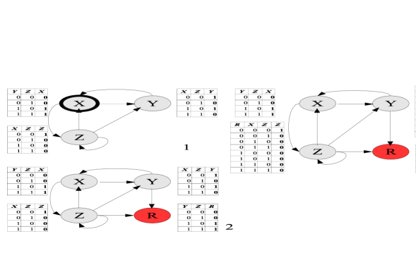
Figure 1: Example of addition of a red node to a RBN $N=3$, $K=2$ (see text for details)

We implemented this algorithm in RBNLab [Gershenson, 2005], and used this software laboratory to measure the overlaps of state space transitions of 1-bit mutant nets with “original” ones, as we add more and more redundant nodes. The mutations consist in flipping a random bit from the lookup table of a randomly selected node. We used normalised Hamming distances (2) to measure the difference $dS$ between state spaces:

$$dS=\frac{1}{2^{n}}\sum\limits_{i}^{2^{n}}H(A_{i}^{t+1},M_{i}^{t+1})$$ (4)

where $A$ is the “original” network, and $M$ is a 1-bit mutant of $A$. $dS$ is calculated by computing one time step in both networks for each initial state $i$. Then, the difference of the states that both networks transitioned is calculated with (2). This is averaged for all initial states ($2^{N}$), and the result reflects how similar the transitions are in both state spaces. If $dS=0$, there is no difference between state spaces, and thus the mutation had no effect. A higher $dS$ reflects a greater effect of the mutation in the state space. There is no correlation of state spaces, i.e. a mutation is maximally catastrophic, when $dS\simeq 0.5$.

A disadvantage of this method is that it is restricted to small networks, since the state space is $2^{N}$. Therefore, for each node that is added to a network, its state space is doubled. Another option would be to have non-exhaustive explorations of state spaces, but this could be misleading. Therefore, we decided to limit our simulations to small networks.

Simulation Results

We can appreciate the average results of ten thousand networks of $N=7$, $p=0.5$ and different $K$ values in Figure 2. We can see that $dS$ decreases exponentially as red nodes are added. We should note that the $dS$ for RBNs without red nodes decreases as $K$ increases. This is because the lookup tables  are doubled each time $K$ is incremented. Thus, a one-bit mutation will have less effect on a network with higher connectivity. To overcome this, we plotted the values of $dS^{K}$ for the same results in Figure 3. We can see that a 1-bit mutation makes $dS^{K}\simeq 0.1$ for networks without red nodes. Clearly the addition of red nodes increases the robustness of the networks. The effect of red nodes is more evident for higher $K$ values, where the network dynamics are more chaotic [Gershenson, 2004].

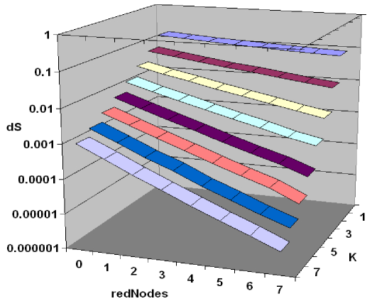
Figure 2: $N=7$, average $dS$ for 10000 networks

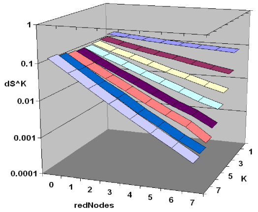
Figure 3: $N=7$, average $dS^{K}$ for 10000 nets

To be certain that the robustness is given by the addition of a red node, and not of any node, we performed simulations with $N=10$. The average values of $dS$ for one thousand networks are shown in Figure 4. We can quickly see that a network with seven white nodes and three red nodes has a lower difference in state spaces than a network with ten white nodes and no red nodes, especially for high values of $K$.

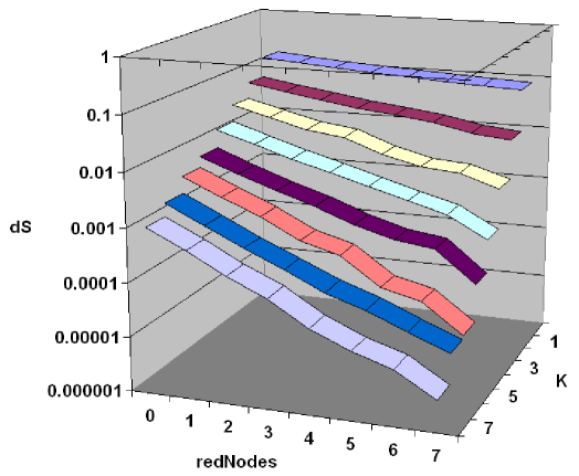
Figure 4: $N=10$, average $dS$ for 1000 networks

We obtained results of RBNs with scale free topology [Aldana, 2003] (data not shown). We observed a similar tendency: as red nodes are introduced in a network, mutants will have less differences in the state space, especially for chaotic networks of high connectivity.

We also obtained results for different updating schemes [Harvey and Bossomaier, 1997, Gershenson, 2002, Gershenson et al., 2003] and both topologies, with similar results (data not shown). The precise effect of redundant nodes on $dS$ does change with the updating scheme: in all cases $dS$ decreases as redundant nodes are added.

Discussion

It is intuitive to assume that redundancy will increase the robustness of a system. If in a minimal program all nodes matter, any mutation will have more drastic effects in the output than in a non-optimal program. This has been seen experimentally in evolvable hardware [Thompson, 1998], where some redundancy allows better evolution of circuits, but too much redundany obstructs it. Still, the goal of our work was to quantify the effect of node redundancy in robustness to mutations in RBN.

Fictitious inputs do not increase the robustness because mutating such inputs can change the logic function. This is not the case for redundant nodes: if a node is mutated, the rest of the network keeps its (partial) function. In other words, mutations in redundant nodes do not propagate through the network, whereas mutations in fictitious inputs do.

From our results we can say that redundancy $smoothens$ rough fitness landscapes [Kauffman, 1993], making evolutionary search potentially feasible in rough fitness landscapes. However, too much redundancy should be detrimental for evolvability, because evolutionary search becomes slower. We can also confirm recent results by Andreas Wagner [Wagner, 2005b] and notice that red nodes increase the neutrality [Kimura, 1983] of the network. A neutral mutation is one that has no effect in the function (or phenotype). As we can see, redundancy of nodes decreases the probability of a mutation causing a change in the functionality. If a mutation occurs in a red node, another node will take its role to perform the old function. From this we can suggest people working with genetic algorithms: if a fitness landscape is too rough to make an evolutionary search on it, then add some redundancy that will smoothen it. Nevertheless, not all types of redundancy will be useful [Harvey and Thompson, 1997].

It could be argued that “useless” redundancy can be added to a state space, i.e. with no effect on the function, and thus would be of no use for evolvability. However, in our RBN approach, a red node cannot be useless, since it is connected to the rest of the network and thus affects its behaviour. Therefore, any red node will have a potential effect on the function of a mutated network: the function of the mutated network will be close to that of the original network, for another node is duplicating the functionality that changed with the mutation. In other words, red nodes provide “useful” redundancy. On the other hand, redundancy given by fictitious links in lookup tables is indeed “useless”: adding fictitious links will have no effect on the mutated network functionality. Still, a general mechanism for deciding wether a certain type of redundancy is useful or not seems to be an open question. In our case, node redundancy does help an evolutionary search in rugged fitness landscapes. To which cases this is applicable remains to be explored. For example, if a fitness landscape is already smooth, adding redundant nodes will be useless to an evolutionary search.

Returning to the original motivation of this work, if Kauffman’s conjecture holds, a random mutation on a “minimal” RBN should produce a $dS\simeq 0.5$. However, we cannot prove if a RBN cannot be reduced or compressed independently of a fixed universal model of computation. Thus, we cannot know if a RBN is minimal. What we have seen is that “less compressible” RBNs, i.e. with no red nodes, have always a higher $dS$. As we add more red nodes, the RBN becomes more compressible, and $dS$ decreases, showing an increase in robustness. As we have seen, the compressibility is directly proportional to the robustness of a network to random mutations. We could extrapolate and induce that if the compressibility could be minimal, then the robustness would be also minimal. The minimal robustness would be given when a single mutation would create $dS\simeq 0.5$, so we can conclude that this corresponds to a minimal compressibility, i.e. a minimal program, even when in theory it is not possible to show this. This does not prove Kauffman’s conjecture, but provides reasonable evidence for its validity.

Conclusions

We have presented an algorithm for introducing redundant nodes in a random Boolean networks. We used this to show that redundancy of nodes increases the mutational robustness of RBNs. This may have advantages for evolvability, depending on the particular problem domain. However, there are other issues that should be also considered for evolvability, such as distributed robustness, degeneracy, and modularity. The relationship between neutrality and redundancy demands further study. This is also the case for redundancy of nodes in larger networks.

Ackwnoledgements

We should like to thank Andrew Wuensche, Adrian Thompson, Miguel Garvie, Tatiana Kalganova, Cosma Shalizi, and Inman Harvey for interesting discussions and comments. C.G. was partly supported by the Consejo Nacional de Ciencia y Teconolgía (CONACyT) of México.

References

- Aldana, 2003 Aldana, M. (2003). Boolean dynamics of networks with scale-free topology. Physica D, 185(1):45–66.
- Aldana-González et al., 2003 Aldana-González, M., Coppersmith, S., and Kadanoff, L. P. (2003). Boolean dynamics with random couplings. In Kaplan, E., Marsden, J. E., and Sreenivasan, K. R., editors, Perspectives and Problems in Nonlinear Science. A Celebratory Volume in Honor of Lawrence Sirovich. Springer Applied Mathematical Sciences Series.
- Chaitin, 1975 Chaitin, G. J. (1975). Randomness and mathematical proof. Scientific American, 232(5):47–52.
- Cook, 2004 Cook, M. (2004). Universality in elementary cellular automata. Complex Systems, 15(1):1–40.
- Fernández and Solé, 2004 Fernández, P. and Solé, R. (2004). The role of computation in complex regulatory networks. In Koonin, E. V., Wolf, Y. I., and Karev, G. P., editors, Power Laws, Scale-Free Networks and Genome Biology. Landes Bioscience.
- Foster et al., 2005 Foster, D. V., Kauffman, S. A., and Socolar, J. E. S. (2005). Network growth models and genetic regulatory networks. arXiv q-bio.MN/0510009.
- Gardner, 1983 Gardner, M. (1983). Wheels, Life, and Other Mathematical Amusements, chapter 20-22. W. H. Freeman.
- Gershenson, 2002 Gershenson, C. (2002). Classification of random Boolean networks. In Standish, R. K., Bedau, M. A., and Abbass, H. A., editors, Artificial Life VIII: Proceedings of the Eight International Conference on Artificial Life, pages 1–8. MIT Press.
- Gershenson, 2004 Gershenson, C. (2004). Introduction to random boolean networks. In Bedau, M., Husbands, P., Hutton, T., Kumar, S., and Suzuki, H., editors, Workshop and Tutorial Proceedings, Ninth International Conference on the Simulation and Synthesis of Living Systems (ALife IX), pages 160–173, Boston, MA.
- Gershenson, 2005 Gershenson, C. (2005). RBNLab. http://rbn.sourceforge.net.
- Gershenson et al., 2003 Gershenson, C., Broekaert, J., and Aerts, D. (2003). Contextual random Boolean networks. In Banzhaf, W., Christaller, T., Dittrich, P., Kim, J. T., and Ziegler, J., editors, Advances in Artificial Life, 7th European Conference, ECAL 2003 LNAI 2801, pages 615–624. Springer-Verlag.
- Harvey and Bossomaier, 1997 Harvey, I. and Bossomaier, T. (1997). Time out of joint: Attractors in asynchronous random Boolean networks. In Husbands, P. and Harvey, I., editors, Proceedings of the Fourth European Conference on Artificial Life (ECAL97), pages 67–75. MIT Press.
- Harvey and Thompson, 1997 Harvey, I. and Thompson, A. (1997). Through the labyrinth evolution finds a way: A silicon ridge. In Higuchi, T., Iwata, M., and Weixin, L., editors, Proceedings of the First International Conference on Evolvable Systems: From Biology to Hardware, volume 1259 of LNCS, pages 406 – 422. Springer-Verlag.
- Huang and Ingber, 2000 Huang, S. and Ingber, D. E. (2000). Shape-dependent control of cell growth, differentiation, and apoptosis: Switching between attractors in cell regulatory networks. Exp. Cell Res., 261:91–103.
- Kauffman, 1969 Kauffman, S. A. (1969). Metabolic stability and epigenesis in randomly constructed genetic nets. Journal of Theoretical Biology, 22:437–467.
- Kauffman, 1993 Kauffman, S. A. (1993). The Origins of Order. Oxford University Press.
- Kauffman, 2000 Kauffman, S. A. (2000). Investigations. Oxford University Press.
- Kauffman, 2004 Kauffman, S. A. (2004). The ensemble approach to understand genetic regulatory networks. Physica A: Statistical Mechanics and its Applications, 340(4):733–740.
- Kimura, 1983 Kimura, M. (1983). The Neutral Theory of Molecular Evolution. Cambridge University Press, Cambridge.
- Lewin, 2000 Lewin, B. (2000). Genes VII. Oxford University Press.
- Nowak et al., 1997 Nowak, M. A., Boerlijst, M. C., Cooke, J., and Maynard Smith, J. (1997). Evolution of genetic redundancy. Nature, 388:167–171.
- Simon, 1996 Simon, H. A. (1996). The Sciences of the Artificial. MIT Press, 3rd edition.
- Thompson, 1998 Thompson, A. (1998). Hardware Evolution: Automatic Design of Electronic Circuits in Reconfigurable Hardware by Artificial Evolution. Distinguished dissertation series. Springer-Verlag.
- von Neumann, 1956 von Neumann, J. (1956). Probabilistic logics and the synthesis of reliable organisms from unreliable components. In Shannon, C. and McCarthy, J., editors, Automata Studies, Princeton. Princeton University Press.
- von Neumann, 1966 von Neumann, J. (1966). The Theory of Self-Reproducing Automata. University of Illinois Press. Edited by A. W. Burks.
- Wagner, 2004 Wagner, A. (2004). Distributed robustness versus redundancy as causes of mutational robustness. Technical Report 04-06-018, Santa Fe Institute.
- Wagner, 2005a Wagner, A. (2005a). Robustness and Evolvability in Living Systems. Princeton University Press, Princeton, NJ.
- Wagner, 2005b Wagner, A. (2005b). Robustness, neutrality, and evolvability. FEBS Letters, 579:1772–1778.
- Watson and Pollack, 2005 Watson, R. A. and Pollack, J. A. (2005). Modular interdependency in complex dynamical systems. Artificial Life, 11(4):445–457.
- Wuensche, 1998 Wuensche, A. (1998). Discrete dynamical networks and their attractor basins. In Standish, R., Henry, B., Watt, S., Marks, R., Stocker, R., Green, D., Keen, S., and Bossomaier, T., editors, Complex Systems ’98, pages 3–21, University of New South Wales, Sydney, Australia.