Pinning and depinning of a classic quasi-one-dimensional Wigner crystal in the presence of a constriction.

Abstract

We studied the dynamics of a quasi-one-dimensional chain-like system of charged particles at low temperature, interacting through a screened Coulomb potential in the presence of a local constriction. The response of the system when an external electric field is applied was investigated. We performed Langevin molecular dynamics simulations for different values of the driving force and for different temperatures. We found that the friction together with the constriction pins the particles up to a critical value of the driving force. The system can depin elastically or quasi-elastically depending on the strength of the constriction. The elastic (quasi-elastic) depinning is characterized by a critical exponent $\beta\sim 0.66$ ($\beta\sim 0.95$). The dc conductivity is zero in the pinned regime, it has non-ohmic characteristics after the activation of the motion and then it is constant. Furthermore, the dependence of the conductivity with temperature and strength of the constriction was investigated in detail. We found interesting differences between the single and the multi-chain regimes as the temperature is increased.

I INTRODUCTION

In the last years the interest in mesoscopic systems consisting of interacting particles in low dimensions or confined geometries has seen a sustained growth. A class of quantum anisotropic systems exhibiting “stripe” behavior appears in the quantum Hall regime qhestripes , in charge density waves (CDW) fogle , in manganite oxides and high-T_c superconductors hightc where strong electronic correlations are responsible for the formation of these inhomogeneous phases. Another class of confined quasi one-dimensional (Q1D) geometries appears in different fields of research and some typical and important examples from the experimental point of view are: ordered electrons on microchannels filled by liquid Helium glasson , microfluidic devices whitesides , colloidal suspensions zahn and confined dusty plasma chu . On the atomic scale a chain-like system was found in compounds such as ${Hg}_{3-\delta}AsF_{6}$ brown and in low dimensional systems formed on surfaces segovia . These kinds of interacting systems, which tend to form periodic or ordered structures when the density of particles and the temperature are low enough (i.e. Wigner crystallization wigner ; andrei ), can exhibit a remarkable variety of complex phenomena when they are driven by an external force. Many of these phenomena, which arise from the interplay between periodicity, disorder, nonlinearities and driving, are still poorly understood or even unexplored. For numerous such experimental systems, transport experiments charalambous ; bhattacharya ; ryu are a useful way to probe the physics (and sometimes the only way when direct methods, e.g. imaging, are not available). It is thus an interesting and challenging problem to obtain a quantitative description of their non-linear dynamics. One striking property exhibited by all these systems is pinning, i.e. at low temperature there is no macroscopic motion unless the applied force $f$ reaches a threshold critical value $f_{c}$. There is a quite extensive literature about the dynamical properties near the depinning threshold dep1 ; dep2 ; dep3 , mostly in the context of CDW cdw1 ; cdw2 ; cdw3 .

The aim of this paper is to provide a description of the properties of a Q1D Wigner crystal in the presence of a local constriction potential, thermal noise and an external driving force. Most of the previous theoretical and experimental works are on moving 2D or 3D lattices and glasses (see Ref. giamarchi and references therein). The effect of confinement into a mesoscopic channel has not yet been deeply investigated.

Our classical model is very ductile because of its scalability and it is suitable for the description of diverse confined systems, as electrons on liquid helium, colloids and complex plasmas. We should stress that the classical approach, which is naturally valid in the case of colloids and complex plasmas because of the microscopic size of the particles, is still valid for pure quantum objects as electrons when they exhibit Wigner crystallization. In the crystal phase the electrons become localized, and thus distinguishable. In this case the De Broglie thermal length $\lambda_{D}$ is much smaller than the interparticle spacing, hence the quantum aspect of the original fermionic problem does not play a crucial role and the classical treatment for the system is an accurate one. Several generic aspects of the present model without a constriction and in the linear regime were recently investigated by the present authors piacente .

A narrow channel with a constriction can be readily realized in a colloidal system or in a dusty plasma. Additionally the problem we deal with could also be of interest in nanoscale wires. Flux-line-lattice flow has been studied in a novel superconducting devices containing straight, nanometer-scale, weak-pinning channels in a strong-pinning environment pruy . By introducing a constriction into the weak-pinning channels many features of the model we propose can be investigated experimentally.

The paper is organized as follows: we first give in Sec. II an overview of the model and of the numerical methods used. In Sec. III we describe the zero temperature phase diagram in the absence of any external driving force, stressing the differences in the ground state configurations near the constriction. Sec. IV is devoted to the study of the dynamics of the system, in particular we concentrate on the velocity vs applied driving force curves and on the conductivity. In Sec. V we discuss the interplay between driving force, thermal disorder and constriction potential, focusing on the difference between the single chain and multi-chain regime. In Sec. VI we comment on the analogies and differences with the case of moving lattices and glasses and other models in which quenched disorder or pinning potentials are present. Finally we conclude in Sec. VII.

II MODEL AND METHODS

The system consists of an infinite number of classical identical particles with charge $q$ and mass $m$, moving in a plane with coordinates $\vec{r}=(x,y)$. The particles interact through a screened Coulomb (Yukawa-type) potential, where the screening length $\lambda$ is an external parameter. We impose a parabolic confining potential in one direction, namely in the $y$-direction, and a constriction potential with Lorentzian shape centered in the origin of the axes. The Hamiltonian of the system is given by:

$$\begin{split}H=&\frac{q^{2}}{\epsilon}\sum_{i>j}\frac{\exp(-|\vec{r_{i}}-\vec{r_{j}}|/\lambda)}{|\vec{r_{i}}-\vec{r_{j}}|}\\ &+\sum_{i}\frac{1}{2}m{\omega_{0}}^{2}{y_{i}}^{2}+\sum_{i}\frac{V_{0}}{1+\alpha^{2}{x_{i}}^{2}},\end{split}$$ (1)

where $\epsilon$ is the dielectric constant of the medium the particles are moving in, $\omega_{0}$ measures the strength of the confining potential, $V_{0}$ is the maximum of the potential of the constriction which has a full width at half maximum $2/\alpha$. Introducing a suitable system of units, the Hamiltonian can be rewritten in a dimensionless form. We define: $r_{0}=(2q^{2}/m\varepsilon\omega_{0}^{2})^{1/3}$ and $E_{0}=(m\omega_{0}^{2}q^{4}/2\varepsilon^{2})^{1/3}$ as unity of length and energy, respectively. After using dimensionless units the Hamiltonian takes the form:

$$\begin{split}H^{\prime}=&\sum_{i>j}\frac{\exp(-\kappa|\vec{r^{\prime}_{i}}-\vec{r^{\prime}_{j}}|)}{|\vec{r^{\prime}_{i}}-\vec{r^{\prime}_{j}}|}\\ &+\sum_{i}{y^{\prime}_{i}}^{2}+\sum_{i}\frac{V^{\prime}_{0}}{1+\alpha^{\prime 2}x^{\prime 2}},\end{split}$$ (2)

where $H^{\prime}=H/E_{0}$, $\kappa=r_{0}/\lambda$, $\overrightarrow{r}^{\prime}=\overrightarrow{r}/r_{0}$, $V^{\prime}_{0}=V_{0}/E_{0}$ and $\alpha^{\prime}=r_{0}\alpha$.

This transformation is particularly interesting because now the Hamiltonian no longer depends on the mass of the particles, the dielectric constant of the medium and the frequency of the parabolic confinement, that is it is independent of the specifics of the system under investigation. The dimensionless time and temperature, which are essential quantities in what follows, are respectively $T^{\prime}=T/[k_{B}(m\omega_{0}^{2}q^{4}/2\varepsilon^{2})^{1/3}]$ and $\tau=t\omega_{0}$.

The zero temperature configurations for different densities, namely different number of particles, and different values of the parameters in the Hamiltonian were calculated by the Monte Carlo (MC) technique using the standard Metropolis algorithm as it was done in Ref. piacente . We have allowed the system to approach its equilibrium state at some temperature $T$, after executing $10^{5}\div 10^{6}$ Monte Carlo steps. In order to reach the $T=0$ equilibrium configuration the technique of simulated annealing was used: first the system was heated up and then cooled down to a very low temperature. We introduced periodic boundary conditions along the $x$-direction in order to simulate an infinite long wire. Typically a simulation cell of length $L=100$ (in dimensionless units) centered around the origin of the axis was used. This choice was motivated by the fact that for larger $L$ the changes in static and dynamical properties are negligible, especially for $\alpha^{\prime}\geq 0.5$ and $\kappa\geq 1$.

Because of the presence of the constriction we found many more metastable states, which complicates the numerical approach. We will elaborate on this point in the next section.

After reaching the $T=0$ equilibrium configuration, we introduced an external electrical field in the $x$-direction, or in other words we considered the effect of an external driving force $f$ and calculate the transport properties of the system. We also considered the effect of temperature and thermal noise, coupling the system to additional degrees of freedom nose ; hoover or to a heat bath. The Langevin dynamics kubo is the most appropriate one to include such effects. The Langevin equations for the $x$ and $y$ components of motion in dimensionless units are respectively:

$$\begin{split}\frac{d^{2}{x^{\prime}_{i}}}{d{\tau}^{2}}=&-\gamma\frac{dx^{\prime}_{i}}{d\tau}-\frac{1}{2}\sum_{j}\frac{\partial}{\partial x^{\prime}_{i}}\frac{\exp(-\kappa|\vec{r^{\prime}_{i}}-\vec{r^{\prime}_{j}}|)}{|\vec{r^{\prime}_{i}}-\vec{r^{\prime}_{j}}|}\\ &+\frac{V^{\prime}_{0}\alpha^{\prime 2}x^{\prime}_{i}}{(1+\alpha^{\prime 2}{x^{\prime}_{i}}^{2})^{2}}+\xi_{x}(T^{\prime})+f\end{split}$$ (3a)

$$\begin{split}\frac{d^{2}{y^{\prime}_{i}}}{d{\tau}^{2}}=&-\gamma\frac{dy^{\prime}_{i}}{d\tau}-\frac{1}{2}\sum_{j}\frac{\partial}{\partial y^{\prime}_{i}}\frac{\exp(-\kappa|\vec{r^{\prime}_{i}}-\vec{r^{\prime}_{j}}|)}{|\vec{r^{\prime}_{i}}-\vec{r^{\prime}_{j}}|}\\ &-y^{\prime}_{i}+\xi_{y}(T^{\prime})\end{split}$$ (3b)

where $\gamma$ is the friction coefficient, which is an external parameter as well as $\kappa$, and $\vec{\xi}(T^{\prime})$ is a random force, reproducing the thermal noise, with zero average and standard deviation

$$\langle\xi_{ir}(\tau)\xi_{js}(\sigma)\rangle=\gamma T^{\prime}\delta_{ij}\delta_{rs}\delta(\tau-\sigma).$$

where $(r,s)\equiv(x,y)$. The driving force $f$ and the random force $\xi$ are measured in units of $m\omega_{0}^{2}r_{0}$, while the friction coefficient $\gamma$ is measured in units of $\omega_{0}$. We used the same simulation cell and the same boundary conditions as in the case of the MC simulations. It should be noticed that in the case of colloids reichhardt or vortices in type II superconductors cao the motion is overdamped and Eqs. (3a) and (3b) are simplified: the hydrodynamic interactions can be neglected and Eqs. (3a) and (3b) reduce to a system of coupled first order differential equations.

We considered here the more general problem, including also the hydrodynamic terms. In order to integrate the equations of motion we used a quasi-symplectic algorithms of ”leap frog” type mannella1 in the form:

$$\tilde{r}_{i} = r_{i}(t)+\frac{\Delta t}{2}v_{i}(t),$$

$$v_{i}(t+\Delta t) = c_{2}\bigg{[}c_{1}v_{i}(t)+\Delta t\frac{\partial H}{\partial r_{i}}(\tilde{r}_{i})+d_{1}\eta_{i}\bigg{]},$$

$$r_{i}(t+\Delta t) = \tilde{r}_{i}+\frac{\Delta t}{2}v_{i}(t+\Delta t),$$

where $\Delta t$ is the time step, and $\eta_{i}$ are Gaussian variables with standard deviation equal to 1 and average equal to 0; the constants $c_{1}$, $c_{2}$ and $d_{1}$ are given respectively by:

$$c_{1} = 1-\frac{\gamma\Delta t}{2},$$

$$c_{2} = \frac{1}{1+\gamma\Delta t/2},$$

$$d_{1} = \sqrt{\gamma T^{\prime}\Delta t}.$$

It was shown that this integration scheme has a good stability and runs rather fast, furthermore it is well behaved in the limit $\gamma\rightarrow 0$ mannella2 .

The driving force was increased from zero by small increments. A time integration step of $\Delta\tau=0.001$ was used and averages were evaluated during $2\times 10^{5}$ steps after $2\times 10^{6}$ steps for equilibration.

III Ground state configurations

The ground state configuration is the result of competitive effects, that is the electrostatic repulsion, the confining potential that tries to keep the particles close to the $x$ axis and the Lorentzian constriction potential that prevents the particles from settling close to the $y$ axis. In Fig. 1 the contour plots of the sum of both potentials for two different values of $V^{\prime}_{0}$ are shown. Depending on the values of (increasing) $V^{\prime}_{0}$ and (decreasing) $\alpha^{\prime}$ the saddle point at $(x,y)=(0,0)$ becomes more pronounced.

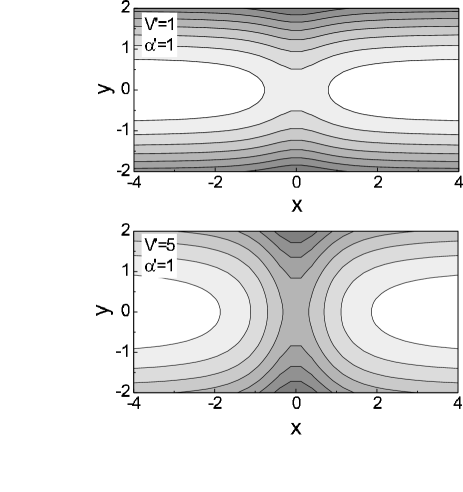
Figure 1: Contour plots of the sum of the confinement and constriction potentials for two different values of the parameters: (a) $V^{\prime}_{0}=1,\alpha^{\prime}=1$, (b) $V_{0}^{\prime}=5,\alpha^{\prime}=1$.

As discussed in Ref. piacente , in the absence of any constriction the charged particles crystallize in a number of chains. Each chain has the same density resulting in a total one-dimensional density $\widetilde{n}_{e}$. If $a$ is the separation between two adjacent particles in the same chain, it is possible to define a dimensionless linear density $\widetilde{n}_{e}=lr_{0}/a$, where $l$ is the number of chains. In the case of multiple chains, in order to have a better packing (or in other words to minimize the interaction energy by maximizing the separation among particles in different chains), the chains are staggered with respect to each other by $a/2$ in the $x$-direction. For low densities the particles crystallize in a single chain; with increasing density a “zig-zag” (continuous) transition zigzag occurs and the single chain splits into two chains. Further increasing the density the four-chain structure is stabilized before the three-chain one. This first four-chain configuration has a relatively small stability range after which it transits to a three chain configuration. For higher values of the density, the four-chain configuration attains again the lowest energy. Then a further increase of $\widetilde{n}_{e}$ will lead to more chains, that is five, six and so on. The structural transitions are all discontinuous (i.e. first order), except the 1 $\rightarrow$ 2 transition.

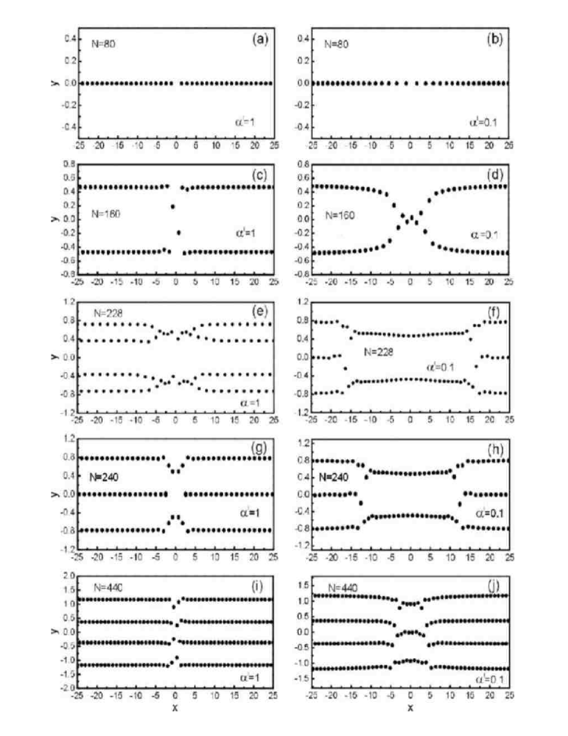
Figure 2: The ground state configuration in the center of the simulation cell for $\kappa=1$, $V^{\prime}_{0}=1$ and different values of the number of particles $N$ in a simulation cell of length $L=100$ and two different values of the constriction width: (a) $N=80,\alpha^{\prime}=1$, (b) $N=80,\alpha^{\prime}=0.1$, (c) $N=160,\alpha^{\prime}=1$, (d) $N=160,\alpha^{\prime}=0.1$, (e) $N=228,\alpha^{\prime}=1$, (f) $N=228,\alpha^{\prime}=0.1$,(g) $N=240,\alpha^{\prime}=1$, (h) $N=240,\alpha^{\prime}=0.1$,(i) $N=440,\alpha^{\prime}=1$, (j) $N=440,\alpha^{\prime}=0.1$. In the case of $\alpha^{\prime}=1$ the effect of the constriction potential is significant only around a narrow region around $(x,y)=(0,0)$, while for $\alpha^{\prime}=0.1$ it is appreciable all along the lenght of the simulation cell. It is interesting to notice that for $\alpha^{\prime}=1$ the reentrant behavior of Ref. piacente , with the four chain arrangement stabilized before the three chain arrangement, is still present, while it is absent for $\alpha^{\prime}=0.1$. For small values of $\alpha^{\prime}$ the configurations are highly inhomogeneous.

In the presence of the constriction potential the ground state configurations are modified near the constriction (see Fig. 2), but the particles are still organized in chains far away from this constriction. Close to the saddle point the particles do not arrange themselves in ordered chains. The particles near the constriction lead to a significant increase of the number of metastable states. Consequently the procedure of simulated annealing has to be more accurate than in the case of the absence of a constriction, which means that several intermediate temperature steps have to be considered. Sometimes the MC simulations do not provide us with the “exact” ground state, as it is seen for instance in Fig. 2 (c), (f) and (j), where the final configurations are not perfectly symmetric with respect to $x$ and $y$, while this is expected because of the symmetry of the Hamiltonian.

When the full width at half maximum of the constriction potential is short enough ($\alpha^{\prime}\geq 0.5$), or in other words the effect of the constriction is significative only in a narrow region around $x=0$, it is still possible to define a local density because the system exhibits a homogeneous spacing among charged particles except in the vicinity of the saddle point. Thus, excluding these regions, it is still meaningful to consider $\widetilde{n}_{e}=lr_{0}/a$, where $l$ is the number of chains. In this case the same chain arrangements, i.e. $1\rightarrow 2\rightarrow 4\rightarrow 3\rightarrow 4\rightarrow 5$ and so on, as in the case where the constriction is absent, is found (see Fig.2 (a), (c), (e), (g) and (i)) with increasing density, but with the difference that all the structural transitions are now discontinuous.

For smaller values of $\alpha$, that is for larger interaction ranges of the constriction potential, the system is highly inhomogeneous and even shows coexistence of different chain phases (see Fig. 2 (d), (f), (h) and (j)). In a certain sense the constriction introduces a local disorder into the system.

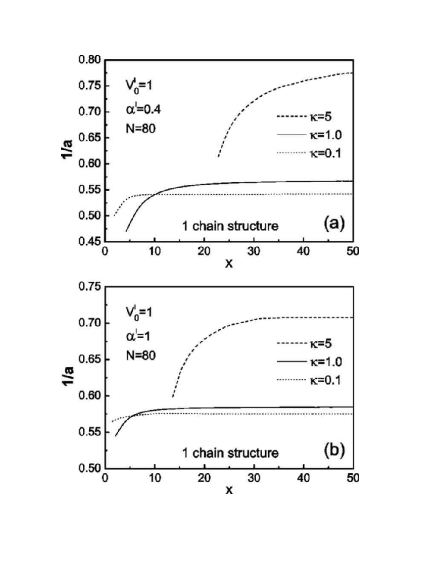
Figure 3: The density as a function of the distance from the origin in the single chain configuration for 80 particles, for a large (a) and short (b) interaction range of the constriction potential. Because of the symmetry of the system around $y=0$ only the results in the right part of the simulation cell are reported.

In order to make these affirmations clearer, we plot in Fig. 3 the inverse interparticle spacing, i.e. the density, in the single chain configuration as a function of the distance from the origin of the coordinates for different values of $\kappa$ and $\alpha^{\prime}$ and $V^{\prime}_{0}=1$. It is evident that the density is an increasing function of the inverse screening length $\kappa$, because the particles can stay closer together as the electrostatic repulsion is weaker. For small values of $\alpha^{\prime}$ the density is an increasing function of the distance over a large range of $x$-values (Fig. 2(a)), while for $\alpha^{\prime}=1$ (Fig. 2(b)) this range can become very small and the density becomes very quickly independent of $x$. Notice that for $x\rightarrow\infty$ the chain density should become independent of the parameters of the constriction.

IV Dynamical properties

When a constant electrical field $E$ is applied to the system in the $x$-direction, it produces a longitudinal driving force $f$. The charged particles then are pushed along the direction of the driving force. In what follows we consider mainly systems for which $\kappa=1$ and $\gamma=0.2$ , which are typical values for the inverse screening length and friction respectively, encountered in complex plasmas goree . We also fixed the value of $\alpha^{\prime}=1$, that means that we deal with short range constrictions.

The first obviously important quantity to determine is the velocity $v^{\prime}$ as a function of the applied force $f$. In the absence of thermal fluctuations, i.e. $T=0$, and in the absence of the constriction potential, Eqs. (3a) and (3b) become:

$$\frac{d{v^{\prime x}_{i}}}{d{\tau}}=-\gamma{v^{\prime x}_{i}}-\frac{1}{2}\sum_{j}\frac{\partial}{\partial x^{\prime}_{i}}\frac{\exp(-\kappa|\vec{r^{\prime}_{i}}-\vec{r^{\prime}_{j}}|)}{|\vec{r^{\prime}_{i}}-\vec{r^{\prime}_{j}}|}+f;$$ (4a)

$$\frac{d{v^{\prime y}_{i}}}{d{\tau}}=-\gamma{v^{\prime y}}-\frac{1}{2}\sum_{j}\frac{\partial}{\partial y^{\prime}_{i}}\frac{\exp(-\kappa|\vec{r^{\prime}_{i}}-\vec{r^{\prime}_{j}}|)}{|\vec{r^{\prime}_{i}}-\vec{r^{\prime}_{j}}|}-y^{\prime}_{i}.$$ (4b)

Furthermore, because in the equilibrium configuration the net force acting on every particle, due to electrostatic repulsion and confinement, is zero, that is

$$\frac{1}{2}\sum_{j}\frac{\partial}{\partial x^{\prime}_{i}}\frac{\exp(-\kappa|\vec{r_{i}}-\vec{r_{j}}|)}{|\vec{r_{i}}-\vec{r_{j}}|}=0;$$

$$\frac{1}{2}\sum_{j}\frac{\partial}{\partial y^{\prime}_{i}}\frac{\exp(-\kappa|\vec{r_{i}}-\vec{r_{j}}|)}{|\vec{r_{i}}-\vec{r_{j}}|}+y^{\prime}_{i}=0,$$

Eqs. (3a) and (3b) can be ulteriorly simplified and one obtains the uncoupled equations:

$$\frac{d{v^{\prime x}}}{d{\tau}}=-\gamma{v^{\prime x}}+f;$$ (5a)

$$\frac{d{v^{\prime y}}}{d{\tau}}=-\gamma{v^{\prime y}},$$ (5b)

whose stationary solutions are respectively:

$$v^{\prime x}=\frac{f}{\gamma};$$ (6a)

$$v^{\prime y}=0.$$ (6b)

This shows that in the absence of thermal noise and constriction the total effect of the external driving force is a sliding of the ordered structure with a drift velocity which is directly proportional to the driving force and inversely proportional to the friction. More in general, when the leading term in the equation of motion is the driving force, one should expect that the drift velocity is $v^{\prime x}=f/\gamma$, or in other words that the system behaves like a classical two-dimensional Drude conductor drude . This feature has been observed in experiments glasson and in numerical simulations chen . In the presence of a constriction and thermal noise, $v^{\prime x}$ is no longer a linear function of the driving force, as we will discuss in the next subsections.

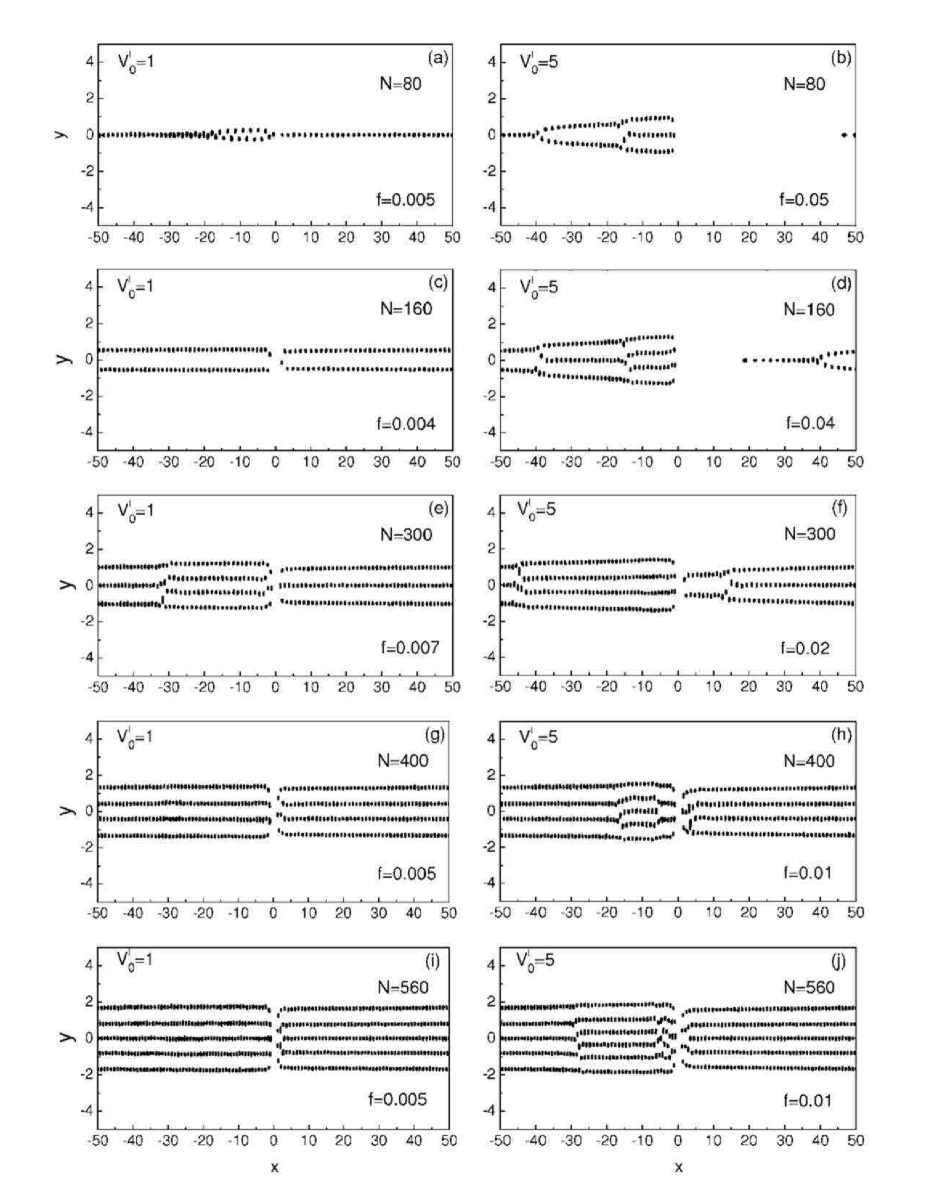
Figure 4: Typical trajectories of the particles when the system is pinned for different number of particles $N$ in a simulation cell of length $L=100$ and different values of the height of the constriction barrier. The plots are for a temperature $T^{\prime}=0.002$, $\kappa=1$ and $\alpha^{\prime}=1$.

IV.1 Pinning

The system is pinned until the applied driving force reaches a threshold value $f_{c}$. The pinned structures in the presence of the driving force show substantial differences with the ground state configurations in the absence of a driving force. The particles move into the direction of the driving force and accumulate in front of the constriction, that exerts a force, which is opposite to the driving force. If $f<f_{c}$, new static configurations are reached, in which the electrostatic repulsion and the repulsive force due to the constriction balance the driving force. The situation is depicted in Fig. 4, where the driving force is in the positive direction of the $x$ axis. In the case of low constriction barrier height, the chain structures are relatively homogeneous, although the inter-chain distance is smaller at the left than at the right of the constriction because of the external drive. In the case of high constriction barrier, the chain structures are no longer homogeneous. As can be seen in Fig. 4, different number of chains can coexist in the same configuration. Since the energy to overwhelm the barrier is quite large, the particles tend mainly to accumulate at $x<0$, which produces a density gradient and consequently a splitting into a larger number of chains where the density is larger, because obviously in such a case the electrostatic repulsion among particles is larger.

It should be noticed that the nature of pinning for the system under investigation is different from the pinning often studied in literature for e.g. colloidal systems and vortex lattices. In these cases the pinning is the result of some kind of disorder (in most cases quenched disorder) or, in other words, the effect of the substrate. It is introduced into the system and modeled as randomly placed point-like pinning centers producing an attractive gaussian potential koshelev ; chen ; cao1 ; cao2 ; brandt or as randomly placed parabolic traps reichhardt . In our case, the pinning is the effect of a constraint, the particles have not enough energy to overcome the constriction barrier and consequently there is no net motion. We also investigated the case of negative $V^{\prime}_{0}$, i.e. a single Lorentzian potential well. In that case we still observed pinning, but without the formation of highly inhomogeneous structures or, in other words, without the accumulation of many particles in the direction of the driving force. In the case of a negative Lorentzian potential the same chain configurations are preserved along the simulation cell length even in the case of a large depth of the potential well. In the case of CDW the pinning potential can be either attractive or repulsive, indeed the the sign of the potential can be converted by changing the phase of the CDW by $\pi$. In what follows we will limit ourselves to positive $V^{\prime}_{0}$.

In Fig. 4, the trajectories of the particles are reported for a temperature $T^{\prime}=0.002$, well below the melting temperature. It is interesting to study for a fixed number of particles and for a fixed temperature how by increasing the driving force the configurations change. The variation of the density along the constriction is shown in Fig. 5 for different values of the external driving force for a constriction height of $V^{\prime}_{0}=5$ and width $\alpha^{\prime}=1$. Increasing the driving force more and more particles accumulate to the left of the constriction barrier in the direction of the driving force, corresponding to larger and larger densities. The density $\widetilde{n}_{e}$ has a discontinuity at the constriction. For low values of the driving force, except in the vicinity of the constriction, $\widetilde{n}_{e}$ is almost constant. But for larger values of the driving force it is always an increasing function of the distance along the simulation cell, except close to the constriction.

Figure 5: The density as a function of the distance along the simulation cell for different values of the driving force and for a temperature $T^{\prime}=0.002$.

Increasing $T^{\prime}$, we observed larger and larger oscillations of the particles until the system is melted. As already reported in Ref. piacente , also in this case we observed larger oscillations in the $x$-direction than in the $y$-direction, which is evidently a combined effect of the confining potential and the nature of the interparticle interaction. In the case of high temperature, close to the solid-liquid transition, and mainly in the case of large $V^{\prime}_{0}$ the arrangements of the particles are slightly different from the ones shown in Fig. 4. Because high values of $V^{\prime}_{0}$ in combination with the driving force produce a density gradient in the chain-like structures, the melting is not homogeneous, with the coexistence of solid and liquid regions. It is beyond the aim of the present paper to discuss how the driving force induces local melting of the system.

The critical force $f_{c}$ is evidently a function of the temperature $T^{\prime}$, it decreases with increasing temperature, that is the thermal motion aids the net motion of the particles. The critical force is also a function of the density, i.e. the number of particles. In our simulations we observed that for larger densities $f_{c}$ becomes smaller.

IV.2 Depinning

When the driving force $f$ is larger than the threshold $f_{c}$, the system exhibits Q1D flow. In Fig. 6 some typical trajectories of the depinned particles are reported, for $T^{\prime}=0.002$ and different values of $f$ just above $f_{c}$.

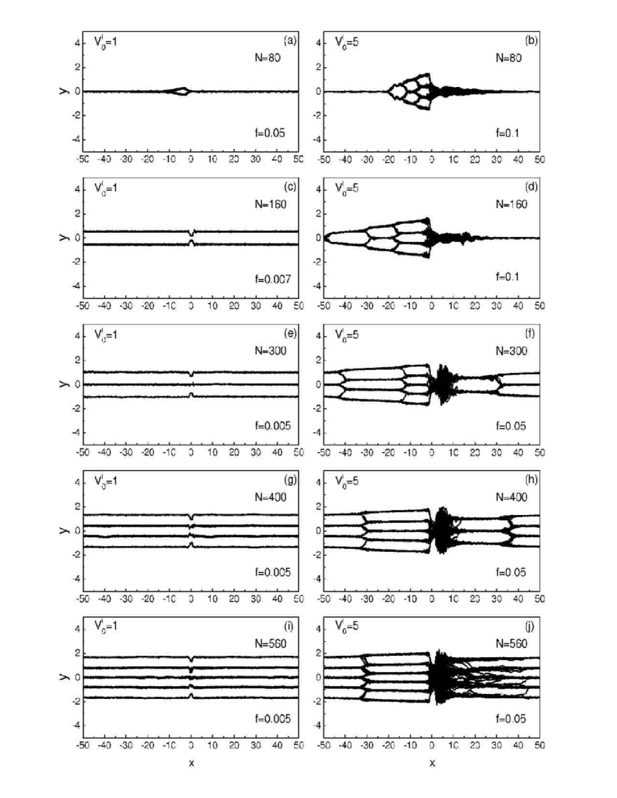
Figure 6: Typical trajectories of the particles when the system is depinned for different densities and different values of the height of the constriction barrier. The plots are for a temperature $T^{\prime}=0.002$, $\kappa=1$ and $\alpha^{\prime}=1$.

The first interesting observation is that the driven system does not break up into pinned and flowing regions, as observed in experiments and simulations of superconducting vortices tanomura ; jensen ; olson or colloids reichhardt , or, in other words, the chain-like system under investigation does not exhibit plastic depinning. Once the driving force overwhelms the critical threshold $f_{c}$, all the particles move together. The depinning can be either elastic or quasi-elastic depending on the height of the constriction barrier. In the case of a low barrier ($V^{\prime}_{0}=1$ in Fig. 6) the particles move such that they keep the same neighbors, thus the system depins elastically. In contrast in the case of a high barrier ($V^{\prime}_{0}=5$ in Fig. 6) a complex net of conducting channels is activated and the particles move without keeping their neighbors, that is the depinning is quasi-elastic. The quasi-elastic depinning is a feature closely related to the low dimensionality of the system and to the fact that we are considering a single constriction. We found that quasi-elastic depinning appears when the strength of the constriction potential is increased. In other infinite 2D systems of driven particles or vortices, where several pinning centers are present, a crossover from elastic to plastic depinning with increasing strength of the pinning potential occurs (see e.g. Ref. reichhardt ). We will focus on this problem in the next subsection.

The region after the constriction barrier, as it is evident from the trajectory patterns, shows features that deserve a deeper investigation in the case of high values of $V^{\prime}_{0}$. In Fig. 6 for $V^{\prime}_{0}=5$ we found that at the right of the constriction some noise is present and the particles flow disorderly. In order to explain this behavior we investigated the distributions of the $x$ and $y$ components of the velocity in narrow strips along the simulation cell length. We concentrated our attention on a system of $N=400$ particles at $T^{\prime}=0.002$, with $\kappa=1$, $V^{\prime}_{0}=5$ and $\alpha^{\prime}=1$. The results are reported in Fig. 7.

It is evident that $v_{y}$ is always normally distributed with average equal to zero, as expected, because it receives contributions mainly from thermal noise, which is gaussian. The distribution of $v_{x}$ is still gaussian, but centered around a value $<v_{x}>\neq 0$ because of the external driving force, except in the neighborhood of the constriction where the strong interaction with the barrier gives a non-gaussian profile to it. What is interesting is the fact that the velocity above the depinning threshold has a pronounced gradient in the $x$-direction. From Fig. 7, it is clear that approaching the constriction from the left side the particles are slowed down; they receive a sudden acceleration when they pass the constriction barrier, then the velocity has a maximum in the right neighborhood of the constriction and finally it slows down again when approaching the edge of the simulation cell. In order to explain these highly non linear features, it is helpful to look at the profile of the force due to the constriction potential (see Fig. 8). This force has a significative magnitude only in a narrow region around $x=0$. For $x<0$ it acts oppositely to the driving force, while for $x>0$ it enhances the driving force. There are two maxima for the intensity of the force located at $x=\pm 1/\sqrt{3}$ and it is zero at the origin of the axis. Therefore, when the particles approach the constriction they start to feel this decelerating force and slow down. Because the system is strongly interacting the deceleration is seen not only in the left neighborhood of the barrier, but in a wider region. At $x=0$ the force is zero, for $x>0$ close to the constriction the force quickly increases and adds to the driving force, so the particles experience a sudden acceleration which produces a large velocity. After that the particles are accelerated only by the driving force and start to feel the effect of the particles on the opposite side of the simulation cell because of the periodic boundary conditions, so the velocity decreases again. In the case of low constriction barriers or large driving forces the $x$ components of the velocity are more homogenously distributed along the simulation cell. From the width of the velocity distribution it is possible to define an “effective temperature”. According to the equilibrium probability factor

$$P\propto\exp{\bigg{[}-\bigg{(}\frac{mv_{x}^{2}}{2k_{B}T_{eff}^{x}}+\frac{mv_{y}^{2}}{2k_{B}T_{eff}^{y}}\bigg{)}\bigg{]}},$$

where $T_{eff}^{x}$ and $T_{eff}^{y}$ take into account also the contributions due to the potential energy, the fluctuations of the velocity components are related to the effective temperature by:

$$T^{x}_{eff}={m<{(v^{\prime}_{x}-<v^{\prime}_{x}>)}^{2}>}/{k_{B}},$$

$$T^{y}_{eff}={m<{(v^{\prime}_{y}-<v^{\prime}_{y}>)}^{2}>}/{k_{B}}.$$

In our dimensionless units and our specific case this yields:

$$T^{\prime x}_{eff}=2<{(v^{\prime}_{x}-<v^{\prime}_{x}>)}^{2}>,$$

$$T^{\prime y}_{eff}=2<{v^{\prime}_{y}}^{2}>,$$

respectively. The calculated effective temperatures are reported in Table I.

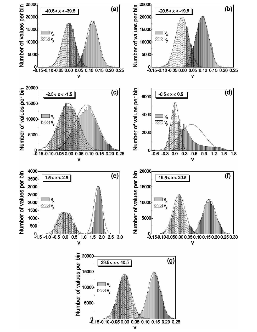
Figure 7: The $v_{x}$ and $v_{y}$ distributions along the simulation cell length for a system of $N=400$ particles, for $\kappa=1$, $V^{\prime}_{0}=5$ and $\alpha^{\prime}=1$ and for a temperature $T^{\prime}=0.002$ and driving force $f=0.05$. The superimposed curves are the normal distribution curves generated using the mean and standard deviation of the data.

It is worth to notice that the effective temperatures are the same as the simulation temperature in the regions far away from the constriction barrier where the velocity fluctuations are nicely described by a normal distribution (see Fig. 7). The effective temperatures $T^{\prime x}_{eff}$ and $T^{\prime y}_{eff}$ increase when approaching the constriction. In the strips $-0.5\leq x\leq 0.5$ and $1.5\leq x\leq 2.5$ both $T^{\prime x}_{eff}$ and $T^{\prime y}_{eff}\gg T^{\prime}$. This is evidently a result of the strong interaction with the barrier which increases significantly the fluctuations in the velocity. Actually, the spreading of the distribution of the velocities is one to two orders of magnitude larger in the constriction region with respect to the regions where the constriction potential is almost zero.

	$T^{\prime x}_{eff}$	$T^{\prime y}_{eff}$
$-40.5\leq x\leq-39.5$	$0.0018$	$0.0020$
$-20.5\leq x\leq-19.5$	$0.0020$	$0.0021$
$-2.5\leq x\leq-1.5$	$0.0060$	$0.0051$
$-0.5\leq x\leq 0.5$	$0.28$	$0.031$
$1.5\leq x\leq 2.5$	$0.14$	$0.26$
$19.5\leq x\leq 20.5$	$0.0024$	$0.0023$
$39.5\leq x\leq 40.5$	$0.0019$	$0.0021$

Table 1: Effective electron temperatures corresponding to the situation of Fig. 6(h) in the different regions studied in Fig. 7.

In the elastic regime the velocity fluctuations could be fitted to a Gaussian distribution both for $v_{x}$ and $v_{y}$, even in the vicinity of the constriction. Around the barrier, the strong interaction effect is felt as an increase of the effective temperature, which is much less pronounced than in the quasi-elastic regime.

Regarding to the noise observed in the trajectory plots, it is essentially due to the fact that the particles merge from the constriction with a relatively large $y$ component of the velocity. As is seen form Fig. 7(d), the distribution of the $v_{y}$ spreads over a quite large range of values while passing the constriction. Indeed, the standard deviation of the $v_{y}$ distribution around $x=0$ is one order of magnitude larger than in the other regions, as already mentioned. This feature is a consequence of the fact that very close to the barrier the constriction force is very small (it is zero at $x=0$), the particles proceed slowly and, thereby, they strongly undergo the effect of the confining potential which accelerates them in the $y$-direction, producing a significant $y$ component of the velocity. This is also confirmed by the fact that passing the constriction barrier a narrowing of the chain structures is always present (see Fig. 6). Notice from Fig. 7(d,e) that the velocity fluctuations are no longer described by a normal thermodynamic equilibrium distribution and that in particular for $v_{x}$ there are large deviations.

Figure 8: The constriction force profile as a function of $x$ for $V^{\prime}_{0}=5$ and $\alpha^{\prime}=1$

As first predicted by Fisher the elastic depinning exhibits criticality fisher and the velocity vs force curves scale as $v=(f-f_{c})^{\beta}$. This scaling has been extensively studied in 2D CDW systems where $\beta=2/3$ narayan ; myers . It is, however, still an open issue whether this exponent is the signature of an universality class and whether it depends on the particle-particle interaction. Actually, in other investigations on elastic depinning of driven colloidal lattices the findings were $\beta\sim 0.5$ pert and $\beta=0.92\pm 0.01$ chen . Other studies on plastic depinning with filamentary or river-like flow have shown a velocity-force curve scaling with $\beta=2.2$ pert , $\beta=1.94\pm 0.03$ reichhardt for colloids, $\beta=2.0$ for electron flow simulations in metallic dots middleton and $\beta=2.22$ for vortex flow in superconductors cao1 .

As pointed out by Le Doussal and Giamarchi, for an infinite size 2D system true elastic depinning is not expected since dislocations and defects, acting as pinning centers, should appear at large scales giamarchi . Both the simulations and the experiments are, however, always for finite size systems and consequently elastic depinning is possible where the distance between dislocations may be larger than the system size.

In Fig. 9, we report the $v-f$ curve in the case of elastic and quasi-elastic depinning for different number of particles, i.e. for different chain arrangements. It should be noticed that the critical exponent does not depend on the number of chains in the system. For all the investigated chain configurations we obtained on average that $\beta\simeq 0.66$ in the case of homogeneous channel flow, that is elastic depinning, and $\beta\simeq 0.95$ in the case of inhomogeneous channel flow, that is quasi-elastic depinning. For negative value of $V^{\prime}_{0}$ we found similar values for the critical exponent in the elastic and quasi-elastic regime. The value of the critical exponent could, therefore, be considered as a clear signature of the kind of depinning. Our results are consistent with the findings on CDW systems and colloids, mentioned before. With increasing temperature but below the melting temperature, we observed a broadening of the conducting channel or some changes in the structure with some chains collapsing (we will provide more details about this point in the next subsection), but no significant dependence of the critical exponent on temperature was found (within our fitting errors).

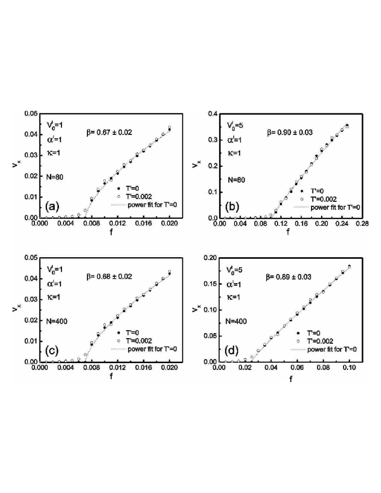
Figure 9: Velocity $v_{x}$ vs applied drive $f$ for the elastic depinning ((a) and (b)), for the quasi-elastic depinning ((c) and (d)) for $\kappa=1$ and $\alpha^{\prime}=1$. The dashed curves are the best fitted power law behavior for $T^{\prime}=0$. At zero temperature the curves exhibit a sudden jump at the depinning threshold, while at finite temperature they are smoother. The critical exponents are independent of the density, i.e. the number of chains.

The question of whether in confined systems there is an universal exponent for elastic and quasi-elastic depinning cannot be answered conclusively. We found that the critical exponent are not affected by the value of $\kappa$, as it can be seen in Table II: going from $\kappa=0.2$ (nearly Coulomb interaction) up to $\kappa=5$ (short range interaction), the value for the critical exponent stays the same. Although we found that the critical behavior is independent of the particle-particle interaction, further investigations with other kind of pinning potentials are required in order to affirm that the elastic, quasi-elastic and plastic depinning belong to different universality classes.

In our simulations neither in case of elastic nor quasi-elastic depinning history dependence was found. The velocity vs applied drive are not hysteretic, and we obtained the same result for increasing and decreasing values of $f$.

Finally, in the case of very small $\alpha$, that is for a wide constriction interaction, because of the density gradient producing the coexistence of different chain structures, we always observed quasi-elastic depinning.

$\kappa$	$V^{\prime}_{0}$	$\beta$	Depinning
$0.2$	$0.25$	$0.68\pm 0.04$	elastic
$0.2$	$1$	$0.70\pm 0.06$	elastic
$0.2$	$5$	$0.95\pm 0.04$	quasi-elastic
$1$	$0.25$	$0.64\pm 0.03$	elastic
$1$	$1$	$0.67\pm 0.02$	elastic
$1$	$5$	$0.92\pm 0.05$	quasi-elastic
$1.5$	$0.25$	$0.63\pm 0.05$	elastic
$1.5$	$1$	$0.68\pm 0.04$	elastic
$1.5$	$5$	$0.95\pm 0.06$	quasi-elastic
$2$	$0.25$	$0.65\pm 0.04$	elastic
$2$	$1$	$0.66\pm 0.03$	elastic
$2$	$5$	$0.96\pm 0.03$	quasi-elastic
$3$	$0.25$	$0.65\pm 0.03$	elastic
$3$	$1$	$0.95\pm 0.06$	quasi-elastic
$3$	$5$	$0.97\pm 0.05$	quasi-elastic
$4$	$0.25$	$0.68\pm 0.04$	elastic
$4$	$1$	$0.94\pm 0.04$	quasi-elastic
$4$	$5$	$0.91\pm 0.05$	quasi-elastic
$5$	$0.25$	$0.67\pm 0.04$	elastic
$5$	$1$	$0.98\pm 0.06$	quasi-elastic
$5$	$5$	$1.02\pm 0.08$	quasi-elastic

Table 2: The critical exponent $\beta$ for different values of the inverse screening length $\kappa$ and the constriction barrier height $V^{\prime}_{0}$.

IV.3 Crossover from elastic to quasi-elastic depinning

It is interesting to investigate the values of $\beta$, or in other word the kind of flow, as a function of $V^{\prime}_{0}$. For colloidal systems a sharp crossover from elastic to plastic depinning was found with increasing strength of the substrate disorder, accompanied by a sharp increase in the depinning critical force reichhardt . Carpentier and Le Doussal studied theoretically the effect of quenched disorder on the order and melting of 2D lattices and found a sharp crossover from the ordered Bragg glass (where there are no defects) to a disordered state carpentier . They also predicted that the depinning threshold increases at the order to disorder transition due to the softening of the lattice, which allows the particles to better adjust to the substrate. A similar mechanism could account for the peak effect observed in vortex matter in superconductors bhatta , in which the depinning threshold rises abruptly with increasing applied magnetic field.

We found a crossover from elastic to quasi-elastic depinning as the barrier height of the constriction is increased. This is analogous to the crossover from the elastic to plastic flow encountered in other systems. As can be seen in Fig. 10, the behavior of $\beta$ as a function of $V^{\prime}_{0}$ is almost step-like, and the crossover takes place in a narrow range of $V^{\prime}_{0}$ values. We also observed increasing values of the critical threshold $f_{c}$. It is beyond the scope of this paper to determine whether the elastic to quasi-elastic crossover is a first or second order transition and how temperature influences this transition. However, the relative smoothness of the curves in Fig. 10 suggests a possible second order transition. Furthermore, the effect of increasing temperature should reasonably result in a shift to lower values of $f_{c}$ or $V^{\prime}_{0}$ for the transition from elastic to quasi-elastic flow.

Figure 10: The critical exponent $\beta$ as a function of the constriction barrier height $V^{\prime}_{0}$ for different values of the inverse screening length: (a)$\kappa=0.2$, (b) $\kappa=1$ and (c) $\kappa=5$. With increasing values of $\kappa$ the crossover region shifts to lower values of $V^{\prime}_{0}$. The solid lines are guides to the eye.

It is evident from Fig. 10 that the crossover shifts towards lower values of the potential barrier as the inverse screening length is increased, which means that the particles with stronger interparticle interactions can flow in a more ordered way.

The values of the critical exponent $\beta$ shown in Fig. 10 can be fitted by the curve $a\tanh{(b(V^{\prime}_{0}-\overline{V}^{\prime}_{0}))+c}$, where $a$, $b$, $c$ and $\overline{V}^{\prime}_{0}$ are the fitting parameters. In particular, the sum $a+c$ gives the value of $\beta$ for the case of quasi-elastic depinning, while the difference $c-a$ gives the value of $\beta$ for the case of elastic depinnig, $\overline{V}^{\prime}_{0}$ can be identified with the value of the constriction height for which the crossover from elastic to quasi-elastic depinning takes place and $b$ is related to the sharpness of the transition or, to be more precise, it is related to the inverse width of the transition region. The results of the fits are reported in Table III.

$\kappa$	$a$	$b$	$c$	$\overline{V}^{\prime}_{0}$
$0.2$	$0.144\pm 0.007$	$2.1\pm 0.6$	$0.799\pm 0.007$	$3.28\pm 0.06$
$1$	$0.131\pm 0.005$	$2.4\pm 0.4$	$0.790\pm 0.004$	$2.90\pm 0.05$
$1.5$	$0.139\pm 0.005$	$3.2\pm 0.4$	$0.796\pm 0.005$	$2.12\pm 0.06$
$2$	$0.143\pm 0.006$	$4.2\pm 1.2$	$0.813\pm 0.006$	$1.78\pm 0.04$
$3$	$0.152\pm 0.005$	$4.8\pm 1.3$	$0.811\pm 0.007$	$1.24\pm 0.05$
$4$	$0.146\pm 0.007$	$5.2\pm 1.3$	$0.802\pm 0.008$	$0.94\pm 0.06$
$5$	$0.160\pm 0.008$	$5.4\pm 1.4$	$0.80\pm 0.01$	$0.61\pm 0.03$

Table 3: The fitting parameters for the crossover curves for different values of the inverse screening length $\kappa$.

As it can be seen from Table III, the constriction height for which the quasi-elastic regime is established is a decreasing function of the inverse screening length $\kappa$, while the sharpness of the transition is an increasing function of $\kappa$ (see also Fig. 11). Again it confirms that for long range interactions the particles can flow more orderly. The errors in the fitting parameters are small for $a$, $c$ and $\overline{V}^{\prime}_{0}$ and relatively large for $b$.

In Fig. 11, the values of $\overline{V}^{\prime}_{0}$ and $b$ as a function of $\kappa$ are reported. The curve $\overline{V}^{\prime}_{0}\equiv\overline{V}^{\prime}_{0}(\kappa)$ is well fitted by a Lorentzian $1/(p+q\kappa^{2})$ with $p=0.302\pm 0.005$ and $q=0.058\pm 0.002$ and the inverse width (see inset of Fig. 11) by the Padé approximation $(g+h\kappa^{2})/(1+l\kappa^{2})$ with $g=1.9\pm 0.2$, $h=1.4\pm 0.4$ and $l=0.23\pm 0.07$.

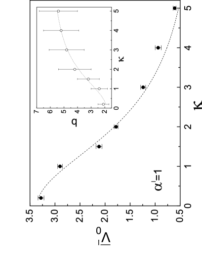
Figure 11: The transition points $\overline{V}^{\prime}_{0}$ as a function of the inverse screening length $\kappa$. The dashed line is the fitting curve $1/(p+q\kappa^{2})$. The inset shows the behavior of the inverse width of the transition region as a function of $\kappa$. The dotted line is the fitting curve $(g+h\kappa^{2})/(1+l\kappa^{2})$.

We should stress that the physics behind the crossover from elastic to quasi-elastic depinning is different from the case of quenched disorder, where with increasing disorder strength the ordered structure is softened and particles can better adjust to the substrate. In our case the accumulation of particles in the vicinity of the constriction barrier and their mutual repulsion give rise for high values of $V^{\prime}_{0}$ to a complex arrangement of conducting channels, in which the nearest neighbors of each particle change, i.e to the impossibility of elastic flow.

IV.4 Conductivity

According to Ohm’s law the current density of a classical system of charged particles is proportional to the applied electric field:

$$\vec{j}=\vec{\sigma}\cdot\vec{E},$$ (7)

where $\vec{\sigma}$ is the specific conductivity. The conductivity can be in general expressed as a second rank tensor. Because of the geometry of the investigated system and because the driving is in the $x$-direction, we are interested only in $\sigma_{xx}$, which we will refer in what follows as simply $\sigma$.

From the definition of $j$ and from Eq. (6a) it follows, in dimensionless units:

$$\sigma^{\prime}=\widetilde{n}_{e}\frac{v^{\prime}_{x}}{f}=\frac{\widetilde{n}_{e}}{\gamma^{\prime}},$$ (8)

where $\sigma^{\prime}=\sigma/(q^{2}/m\omega_{0}r_{0})$. As the definition of total density is not always an accurate one for our system, as mentioned above, we investigated the ratio $v^{\prime}_{x}/f$, which is directly proportional to $\sigma^{\prime}$ through $\widetilde{n}_{e}$ and which is a constant equal to $1/\gamma^{\prime}$, according to Eq. (8). In Fig. 12 the results of our calculations are reported for different values of the friction.

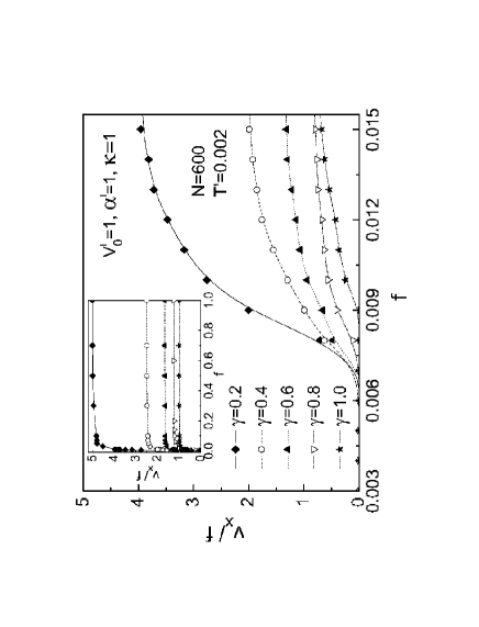
Figure 12: The ratio between velocity and driving force as a function of the drive strength for different values of the friction coefficient. The conductivity is non-Ohmic in a narrow region above the depinning threshold. The inset shows that for larger values of $f$ Ohm’s law is fulfilled with the conductivity as a constant. The curves are guides to the eye.

When the particles are pinned the conductivity is obviously zero. It is interesting to notice that after the depinning threshold, there is a narrow region where the conductivity shows non-Ohmic features, going from zero to the saturation value $1/\gamma^{\prime}$. Afterwards when the drive is the leading effect in the equations of motion, the particles behave as a classical Ohmic conductor. This behavior is independent of the number of particles and of the height of the constriction barrier. For higher values of $V^{\prime}_{0}$ the non-Ohmic conductivity region is enlarged.

Studying the conductivity as a function of temperature some interesting features were observed. We investigated a rather wide range of temperatures from 0.001 to 0.018. From Ref. piacente we know that for the single chain configuration in the absence of driving and constriction potential, the melting temperature is arbitrarily low, while in the multiF-chain configuration it is $T^{\prime}_{m}\sim 0.015$. The results of our calculations, for a driving force $f=0.05$ and for different values of $V^{\prime}_{0}$, are sketched in Fig. 13.

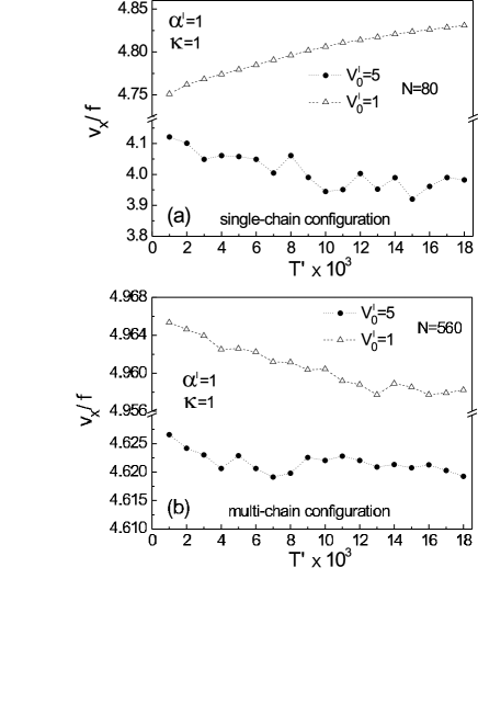
Figure 13: Dependence of the conductivity on the temperature, for (a) a single-chain structure and (b) a multi-chain structure. For weak values of the potential barrier the conductivity of the single-chain structure is an increasing function of temperature, in all the other cases it shows a decreasing trend.

The behavior in the single chain configuration shows substantial differences from the multi-chain one. First of all, for weak values of $V^{\prime}_{0}$, the conductivity is an increasing function of $T^{\prime}$ in the single chain case, while it is decreasing in the multi-chain case. This means that when the number of particles is small, that is the electrostatic interaction is not too strong, the thermal motion aids the particles to overcome the potential barrier and does not act as a disturbance, while in the case of a large number of particles, the possibility of overcoming the barrier is sustained by the electrostatic repulsion and the thermal agitation is a dissipative factor. This is an ulterior confirmation that the dynamics of the system under investigation is a very complex interplay of driving, electrostatic interaction, repulsion from the constriction, thermal fluctuations and confinement.

In general, in a classical model of conduction the conductivity is expected to be a decreasing function of temperature. For large values of the constriction barrier height either in the case of single chain and multi-chain structures, we found that the conductivity is not a monotonic function of temperature, although it shows a decreasing trend. The presence of structure in the $v_{x}/f$ curve vs $T^{\prime}$ can be explained by the fact that with increasing temperature some of the channels formed for high $V^{\prime}_{0}$ can collapse together to form new channels, as mentioned in previous subsection. This is confirmed by the analysis of the configurational energy per particle as a function of temperature, which is plotted in Fig. 14.

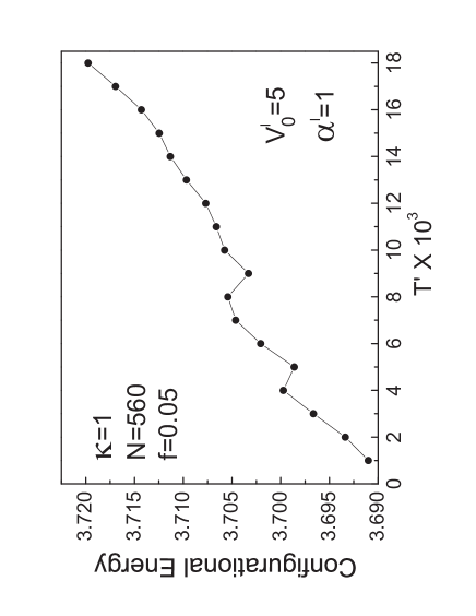
Figure 14: The average configurational energy per particle as a function of the temperature for a multi-chain configuration.

The average potential energy exhibits the same temperature dependance as the conductivity, while in the case of a weak constriction barrier height the configurational energy per particle increases linearly with temperature. Another factor, which is also responsible for that non monotonicity, is the fact that, in the case of high barrier values, a density gradient is present and the melting is not homogenous, thus some parts of the system can be in the liquid state while others are still in the solid state, giving rise to complex phenomena in the transport properties.

V Other Dynamical properties

For high values of the driving force the system shows the phenomenon of dynamical reordering. When the driving force is large the system, even in case of a high constriction barrier, can flow in an ordered channel structure. This is shown in Fig. 15. It is interesting to compare the trajectories of Fig. 15 with the one of Fig. 6(j). Above the depinning threshold (Fig. 6(j)) the channel structures are not homogenous, with increasing the drive (Fig. 15) an ordered moving structure is reached again.

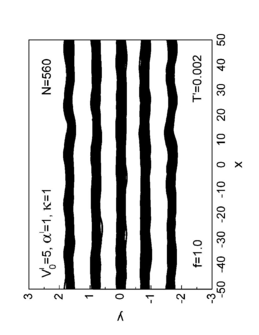
Figure 15: Trajectories of a system of N=560 particles for a high value of the driving force. The five channel structure is attained over the whole wire (cfr. Fig. 7(j)).

This is a well known phenomenon. Indeed, it was observed experimentally for vortex lattices in type II superconductors yaron and for colloids helle . The interplay between dynamical reordering and melting in mesoscopic channels was recently studied experimentally in the case of vortices, providing the first conclusive evidence for a velocity dependent melting transition kes . The dynamical reordering was also investigated theoretically for CDW systems fisher . The dynamical reordering for such systems originates from the fact that the applied driving force tilts the pinning potential thereby reducing the pinning strength. When a large enough force is applied, the particles depin and then flow quite orderly. The same mechanism is responsible for the dynamical reordering of the studied system, with the difference that the tilted potential is in this case the constriciton potential.

It is worth to study the ratio between kinetic and potential energy, averaged at every simulation step, as a function of the temperature. From Fig. 16 it is evident that the kinetic energy increases faster than the configurational energy with temperature, which is an expected result. What is interesting is the fact that the fitting curve is of the type $y=c/(1+dx)$. The fit is excellent with very small errors in the fitting parameters $c$ and $d$.

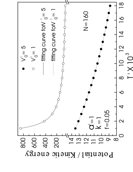
Figure 16: The ratio between potential and kinetic energy per particle as a function of temperature.

Finally, we also investigated the distribution of the velocity $v_{x}$ as a function of the distance from the $x$ axis, or in other words we studied the velocity for each conducting channel when the system flows orderly. Motivated by the experimental findings of Ref. glasson , that for a chain system of electrons on liquid helium, the particles in the external chains have higher velocity than the particles in the internal chains, we tried to clarify whether in our system a similar behavior occurs. Our findings are in contrast with the one of Ref. glasson , actually we found that the internal chains have on average a velocity which is 5% higher than the external chains. However, this discrepancy can be explained by the circumstance that the pinning mechanism are different for the two systems: the coupling between electrons and ripplons in case of Ref. glasson and the constriction potential in our case, and by the fact that the confinement potentials are not exactly the same in the two systems.

VI Comparison with other driven systems

A rather general theory of periodic structures in a random pinning potential under the action of an external driving force was developed by Le Doussal and Giamarchi giamarchi . Their findings were that the periodicity in the direction transverse to the motion leads to a different class of driven system: the moving glasses, with the decay of the translational long-range order as a power law. Similar considerations can be made for our system as well, but with the important difference that because of the confining potential and the constriction potential the periodicity is broken both in the $x$ and $y$-direction. For weak constriction barrier height long-range translational order is present in the $x$-direction, but it is softened when the system is moving and the temperature is increased. For infinite systems one of the consequences of periodicity in the transverse direction to the motion is that particles flow along static channels for uncorrelated and weak disorder and that there are barriers to transverse motion. In our confined system the barriers to transverse motion are an effect resulting from confinement instead of periodicity. Most of the studies on driven lattices or glasses show that, at finite but low temperature, the channels broaden and strong non-linear effects exist in the response to the applied drive, though the asymptotic behavior is found to be linear, which is, indeed, what we found as well.

In infinite moving systems with random pinning centers, depending on the strength of that disorder, two kinds of flow are possible: (i) the elastic one, where all the particles move keeping their neighbors, and (ii) the plastic one, where part of the particles are moving in river-like or filamentary structures and part is pinned. There is a sharp crossover from the elastic to the plastic flow, related to an order-disorder transition. In our system we found that two kinds of flow are possible: (i) the elastic flow, where all the particles move orderly and the nearest neighbors are preserved, and (ii) the quasi-elastic flow, where all the particles move together, but creating a complex net of conducting channels, for which the neighbors are not kept. We also found a continuous crossover from the elastic to quasi-elastic flow. It is important to stress that this difference is closely related to the different pinning potentials considered. To be more precise, in the case we investigated the pinning is due to a constraint rather than an actual pinning potential. That is the reason why we did not observe plastic flow, because particles cannot be strongly attracted and pinned by any pinning center.

It is remarkable that for our system we also found that in the case of elastic depinning the velocity vs driving force curve scales as $v\propto(f-f_{c})^{\beta}$, with $\beta\sim 0.66$, which is in agreement with most of the theoretical and numerical works for infinite systems exhibiting elastic flow, where $\beta=2/3$. Thus, the value of the critical exponent $\beta=2/3$ seems actually the signature of elastic depinning independently of the presence of confinement and the type of pinning potential. Naturally, in order to affirm this definitely more investigations are required with different topologies and potentials. Furthermore, in the case of quasi-elastic depinning we found a critical exponent $\beta\sim 0.95$, which is an intermediate value between the case of elastic and plastic flow, where the experimental findings give $\beta\sim 2$. This leads us to the conclusion that the quasi-elastic depinning is an intermediate regime between elastic and plastic depinning.

Finally, for the elastic regime the previous theoretical investigations followed essential two approaches: (i) elastic theory with renormalization group techniques giamarchi ; carpentier and (ii) perturbation theory in $1/v$ sneddon ; larkin ; schmidt . The first one explains the flowing channel structures and their mutual interactions, while the second one elucidates the $v-f$ characteristics and the criticality in the depinning. Despite the number of experimental and numerical data a detailed theoretical understanding of plastic motion remains still a challenge watson .

VII Conclusions

We studied the ground state and the dynamical properties of a classical Q1D infinite system of particles interacting through a Yukawa-type potential and with a Lorentzian shaped constriction potential. The system is confined in one direction by a parabolic potential. By MC simulations we found that at $T=0$ the particles arrange themselves in a chain-like system, where the number of chains are a function of the number of particles, i.e. the density. Depending on the height and on the interaction range of the constriction barrier, a density gradient in the chain configuration is present near the constriction.

We studied the response of the system when an external driving force is applied in the not confined direction. We performed Langevin molecular dynamics simulations with periodic boundary conditions in the not confined direction and open conditions in the confined direction for different values of the driving force and for different temperatures. We found that the constriction barrier and the friction pins the particles up to a critical value of the driving force. The pinned phase is a new static phase, with particles accumulating in the neighborhood of the constriction and arranging themselves in such a way to balance the external drive. For values of the driving force which are higher than the critical threshold, the particles can overcome the potential barrier and the system depins. We analyzed in detail the depinning phenomenon and we found that the system can depin elastically or quasi-elastically depending on the strength of the constriction potential. The quasi-elastic flow is a new regime, where particles move together without keeping their neighbors.

In the case of elastic flow the chain-like structure, formed at $T=0$ in the absence of external drive, is preserved, while in the case of quasi-elastic flow it is destroyed and a complex net of conducting channels is created. The elastic depinning is characterized by a critical exponent, which is on average $\beta\sim 0.66$ and does not depend on the number of chains. This is in excellent agreement with the theoretical and numerical findings on 2D systems exhibiting elastic depinning. The quasi-elastic depinning state has a critical exponent $\beta\sim 0.95$. We demonstrated that the values of the critical exponent are independent of the range (i.e. screening length) of the interparticle interaction. But the crossover between elastic and quasi-elastic flow depends on the kind of interparticle interaction.

Furthermore, we showed that the dc conductivity is zero in the pinned regime, it has non-Ohmic characteristics after the activation of the motion and then it is constant, in other words the system has a non linear response to the applied drive. The linear regime is attained as the asymptotic behavior. The dependence of the conductivity with temperature and strength of the constriction was also investigated. We found that in the single chain configuration for low height of the constriction, the conductivity is an increasing function of temperature, while in the multi-chain configuration it is a decreasing function, as expected. For high constriction barrier height, the conductivity has no longer a monotonic behavior, although it has a decreasing trend. In these cases some structures are present in the conductivity vs temperature curve, signaling the circumstance that some channels collapse or some parts of the system have already undergone the transition form the solid to the liquid state. Finally, for large values of the external driving force even in the case of high constriction barrier, the particles can flow orderly in a well defined channel structure, because the drive tilts the contriction potential, thus reducing the pinning strength, that is the system exhibits the phenomenon of dynamical reordering.

VIII Acknowledgments

This work was supported in part by the European Community’s Human Potential Programme under contract HPRN-CT-2000-00157 ”Surface Electrons” and the Flemish Science Foundation (FWO-Vl). We thank Dr. I. Schweigert for interesting discussions.

References

- (1) Email address: piacente@ua.ac.be.
- (2) Email address: francois.peeters@ua.ac.be.
- (3) M. P. Lilly, K. B. Cooper, J. P. Eisenstein, L. N. Pfeiffer, and K. W. West, Phys. Rev. Lett. 82, 394 (1999).
- (4) W. Fogle, and H. Perlstein, Phys. Rev. B 6, 1402 (1972).
- (5) E. Dagotto, T. Hotta, and A. Moreo, Physics Reports, 344, 1 (2001);
- (6) P. Glasson, V. Dotsenko, P. Fozooni, M. J. Lea, W. Bailey, G. Papageorgiou, S. E. Andresen, and A. Kristensen, Phys. Rev. Lett. 87, 176802 (2001).
- (7) Yu. Z. Kovdrya, Low Temperature Physics 29, 77 (2003).
- (8) G. M. Whitesides and A. D. Stroock, Physics Today 54, 42 (2001).
- (9) K. Zahn, R. Lenke, and G. Maret, Phys. Rev. Lett. 82, 2721 (1999).
- (10) J. H. Chu and Lin I, Phys. Rev. Lett. 72, 4009 (1994).
- (11) A. Brown, Can. J. Chem. 52, 791 (1974).
- (12) P. Segovia, D. Purdie, M. Hengsberger, and Y. Baer, Nature (London) 402, 504 (1999).
- (13) E. Wigner, Phys. Rev. 46, 1002 (1934).
- (14) E. Y. Andrei, G. Deville, D. C. Glattli, F. I. B. Williams, E. Paris, and B. Etienne, Phys. Rev. Lett. 60, 2765 (1988).
- (15) M. Charalambous, J. Chaussy, and P. Lejay, Phys. Rev. B 45, R5091 (1992).
- (16) S. Bhattacharya and M. J. Higgins, Phys. Rev. Lett. 70, 2617 (1993).
- (17) S. Ryu, M. Hellerqvist, S. Doniach, A. Kapitulnik, and D. Stroud, Phys. Rev. Lett. 77, 5114 (1996).
- (18) D. S. Fisher, Phys. Rev. B 31, 1396 (1985).
- (19) T. Nattermann, S. Stepanow, L. H. Tang, and H. Leschom, J. Phys. I 2, 1483 (1992).
- (20) O. Narayan and D. S. Fisher, Phys. Rev. B 48, 7030 (1993).
- (21) P. B. Littlewood, in Charge Density Waves in Solids: Proceedings, Budapest, 1984, edited by G. Hutiray and J. S lyom (Springer-Verlag, Berlin, 1985).
- (22) L. Sneddon, M. C. Cross, and D. S. Fisher, Phys. Rev. Lett. 49, 292 (1982).
- (23) O. Narayan and D. S. Fisher, Phys. Rev. B 46, 11520 (1992).
- (24) P. Le Doussal and T. Giamarchi, Phys. Rev. B 57, 11356 (1998).
- (25) G. Piacente, I. V. Schweigert, J. J. Betouras, and F. M. Peeters, Solid State Commun. 128, 57 (2003); Phys. Rev. B 69, 045324 (2004).
- (26) A. Pruymboom, P. H. Kes, E. van der Drift, and S. Radelaar, Phys. Rev. Lett. 60, 1430 (1988)
- (27) S. Nose, Prog. Theor. Phys. Supp. 103, 1 (1991).
- (28) W. G. Hoover, Phys. Rev. A 31, 1695 (1985).
- (29) R. Kubo, M. Toda, and N. Hashitume, Non Equilibrium Statistical Mechanics (Springer-Verlag, Berlin, 1992).
- (30) C. Reichhardt and C. J. Olson, Phys. Rev. Lett. 89, 078301 (2002).
- (31) Y. Cao, J. Zhengkuan, and H. Ying, Phys. Rev. B 62, 4163 (2000).
- (32) R. Mannella, Int. J. Mod. Phys. C 13, 1177 (2002).
- (33) R. Mannella, Phys. Rew. E 69, 041107 (2004).
- (34) L. Candido, J. P. Rino, N. Studart, and F. M. Peeters, J. Phys.: Cond. Matt. 10, 11627 (1998).
- (35) P. Drude, Ann. Phys. (Leipzig) 1, 566 (1900).
- (36) J. Chen, Y. Cao, and Z. Jiao, Phys. Rev. E 69, 041403 (2004).
- (37) B. Liu, K. Avinash, and J. Goree, Phys. Rev. Lett. 91, 255003 (2003).
- (38) A. E. Koshelev and V. M. Vinokur, Phys. Rev. Lett. 73, 3580 (1994).
- (39) Y. Cao, Z. Jiao, and H. Ying, Phys. Rev. B 62, 4163 (2000).
- (40) Y. Cao and Z. Jiao, Physica C 321, 177 (1999).
- (41) E. H. Brandt, Phys. Rev. Lett. 50, 1599 (1983).
- (42) A. Tonomura, H. Kasai, O. Kamimura, T. Matsuda, K. Harada, J. Shimoyama, K. Kishio, and K. Kitazawa, Nature (London) 397, 308 (1999).
- (43) H. J. Jensen, A. Brass, and A. J. Berlinsky, Phys. Rev. Lett. 60, 1676 (1988); M. C. Faleski, M. C. Marchetti, and A. A. Middleton, Phys. Rev. B 54, 12427 (1996).
- (44) C. J. Olson, C. Reichhardt, and F. Nori, Phys. Rev. Lett. 81, 3757 (1998).
- (45) D. S. Fisher, Phys. Rev. B 31, 1396 (1995).
- (46) O. Narayan and D. S. Fisher, Phys. Rev. Lett. 68, 3615 (1992).
- (47) C. R. Myers and J. P. Sethna, Phys. Rev. B 47, 11171 (1993).
- (48) A. Pertsinidis and X. S. Ling, Bull. Am. Phys. Soc. 46, 181 (2001);
- (49) A. A. Middleton and N. S. Wingreen, Phys. Rev. Lett. 71, 3198 (1993).
- (50) D. Carpentier and P. Le Doussal, Phys. Rev. Lett. 81, 1881 (1998).
- (51) S. Bhattacharya and M. J. Higgins, Phys. Rev. B 49, 10005 (1994).
- (52) U. Yaron, P. L. Gammel, D. A. Huse, R. N. Kleiman, C. S. Oglesby, E. Bucher, B. Batlogg, D. J. Bishop, K. Mortensen, K. Clausen,C. A. Bolle, and F. DeLaCruz, Phys. Rev. Lett. 73, 2748 (1994).
- (53) M. C. Hellerqvist, D. Ephron, W. R. White, M. R. Beasley, and A. Kapitulnik, Phys. Rev. Lett. 76, 4022 (2003).
- (54) R. Besseling, N. Kokubo, and P. H. Kes, Phys. Rev. Lett. 91, 177002 (2003).
- (55) L. Sneddon, M. C. Cross, and D. S. Fisher, Phys. Rev. Lett. 49, 292 (1982).
- (56) A. I. Larkin and Y. N. Ovchinnikov, Sov. Phys. JEPT 38, 854 (1974).
- (57) A. Schmidt and W. Hauger, J. Low Temp. Phys. 11, 667 (1973).
- (58) J. Watson and D. S. Fisher, Phys. Rev. B 55, 14909 (1997).