Soliton solutions of driven non-linear and higher order non-linear Schrödinger equations

Abstract

We analyse the structure of the exact, dark and bright soliton solutions of the driven non-linear Schrödinger equation. It is found that, a wide class of solutions of the higher order non-linear Schrödinger equation with a source can also be obtained through the above procedure. Distinct parameter ranges, allowing the existence of these solutions, phase locked with their respective sources, are delineated. Conditions for obtaining non-propagating solutions are found to be quite different for both the equations. A special case, where the scale of the soliton emerges as a free parameter, is obtained and the condition under which solitons can develop singularity is pointed out. We also study the highly restrictive structure of the localised solutions, when the phase and amplitude get coupled.

1 Introduction

The externally driven, non-linear Schrödinger equation (NLSE) with a source has been investigated in the context of a variety of physical processes. It arises in the problem of Josephson junction [1], charge density waves [2], twin-core optical fibres [3, 4, 5, 6], plasma driven by rf fields [8] and a number of other problems [9]. As compared to NLSE, which is an integrable system [10], not much is known about the exact solutions of this equation. Perturbative solutions around the stable soliton solutions of NLSE with a source have been studied earlier. Analysis around constant background and numerical investigations [11, 12, 13] have revealed the phenomenon of auto-resonance [14, 15] as a key characteristic of this system, where a continuous phase locking between the solutions of NLSE and the driven field is observed.

In a recent work [16], some of the present authors have devised a procedure based on fractional linear transformation for obtaining exact solutions of this dynamical system. One obtains both localised and oscillatory solutions. Apart from these regular solutions, under certain constraints singular solutions have also been found, implying extreme increase in the field intensity due to self-focussing. This approach is non-perturbative in the sense that, the obtained exact solutions are necessarily of rational type, with both numerator and denominator containing terms quadratic in elliptic functions. However, the exact parameter ranges in which the general solution exhibits bright and dark nature has not been investigated. Considering, the importance of the localised solutions of this physically important dynamical system, the above point needs a systematic study.

The goal of the present paper is to analyse in detail the structure of the most general, localised bright and dark solitons of the NLSE with a source. The parametric restrictions, under which singular structures can form, are obtained. Unlike NLSE, it is observed that dark and bright solitons, depend both on coupling and source strengths. For example, bright solitons can also form in the repulsive regime, if the source strength has positive value. Similarly dark solitons can form in the attractive regime. Conditions which give non-propagating solutions, for driven NLSE, are studied. The possibility, where the phase and amplitude can get related is also investigated. The highly restrictive nature of the resulting dynamics is pointed out. In the process, we also find a large class of solutions to higher order nonlinear Schrödinger equation (HNLSE) with a source, by connecting the solution space of these two equations. HNLSE, which is a generalisation of NLSE, has been proposed by Kodama [17] and Kodama and Hasegawa [18] to describe the propagation of short duration (femtosecond) pulses in optical fibres. The fact that NLSE with a source describes twin-core fibres, under certain conditions [5, 6, 7], motivates us to find exact solution of HNLSE with a source. A possible scenario leading to driven HNLSE is pulse propagation through asymmetric twin-core fibre involving a femtosecond pulse in first core, having anomalous dispersion, and a nanosecond pulse propagating in second core in the normal dispersion regime. Analysis of the solution space of the driven HNLSE shows many interesting features. Non-propagating solutions of driven HNLSE show a much richer structure as compared to NLSE, because of the presence of the higher order terms.

The paper is organised as follows. In the following section, we elaborate briefly on the method of the fractional linear transform for obtaining the solutions of the NLSE with a source. In this section, it is shown that for a large class of solutions, driven HNLSE can also be connected with driven NLSE. Hence, the obtained solutions are also solutions of HNLSE, albeit with different relations among the parameters. The third section is devoted to the investigation of appropriate parameter regimes, characterising bright, dark and singular solutions, and their analysis. In the fourth section, the structure of the solutions space is studied, when the phase and amplitudes are coupled. We then conclude after pointing out the open problems and future directions of work.

2 Analysis of NLSE phase locked with source
and its relation to HNLSE

The equation which we intent to solve is driven NLSE, which is space time dependent, and phase locked with the source:

$$i\frac{\partial\phi}{\partial t}+\frac{\partial^{2}\phi}{\partial x^{2}}+g\mid\phi\mid^{2}\phi+\mu\phi=\kappa e^{i(kx-\omega t)}\quad,$$ (1)

where $g$, $\mu$, $\kappa$, $\omega$ and $k$ are real constants. As we will see later, it can be connected with HNLSE, for a wide class of solutions. We consider the ansatz travelling wave solution in the form,

$$\phi(x,t)=\sigma(\xi)e^{i(kx-\omega t)},$$

where $\xi=\alpha(x-vt)$. Separating the real and imaginary parts of equation (1), one obtains, $v=2k$, from the imaginary part, indicating that in the present case, wave velocity $v$ is controlled by $k$. The real part yields,

$$\alpha^{2}\sigma^{\prime\prime}+g\sigma^{3}+{\epsilon{\sigma}}={\kappa},$$ (2)

where $\epsilon=\omega-k^{2}+\mu$, and prime indicates differentiation with respect to $\xi$. As has been observed earlier [16], this equation can be connected to the equation $f^{\prime\prime}+af+bf^{3}=0$ through the following fractional linear transformation (FT):

$$\sigma(\xi)=\frac{A+Bf(\xi|m)^{2}}{1+Df(\xi|m)^{2}}$$ (3)

where $A$,$B$ and $D$ are real constants, and $f(\xi|m)$ is a Jacobi elliptic function, with the modulus parameter m. We consider the case where, $f({\xi|m})=cn({\xi}|m)$, other cases can be similarly studied. Since the goal is to study the localised solutions, we consider the case with modulus parameter $m=1$, which reduces $cn(\xi)$ to sec hyperbolic of $\xi$. It is worth pointing out that, other solutions involving $sn(\xi)$ and $dn(\xi)$ naturally emerge from the above solution, since the transform involves square of the $cn(\xi)$ function. It should also be mentioned that, in the above fractional transform the second power of the cnoidal functions emerge, as the highest power.

We can see that equation (3) connects $\sigma(\xi)$ to Jacobi elliptic equation, provided $AD{\neq}B$, and the following conditions are satisfied for the localised solutions:

$$A\epsilon+gA^{3}-\kappa=0,$$ (4)

$$2\epsilon AD+\epsilon B+4\alpha^{2}(B-AD)+3gA^{2}B-3\kappa D=0,$$ (5)

$$A\epsilon D^{2}+2\epsilon BD+4\alpha^{2}(AD-B)D$$

$$+6\alpha^{2}(AD-B)+3gAB^{2}-3\kappa D^{2}=0,$$ (6)

$$\epsilon BD^{2}+2\alpha^{2}(B-AD)D+gB^{3}-\kappa D^{3}=0.$$ (7)

Equation (4) in $A$ does not involve $B$ and $D$, which is first solved to get the real $A$. Thus $A$ is determined in terms of $\epsilon$, $\kappa$, and $g$. From equation (5), we determine $D$ in terms of $B$ as, $D=\Gamma B,$ where, $\Gamma=\frac{\epsilon+4\alpha^{2}+3gA^{2}}{4\alpha^{2}A+3\kappa-2\epsilon A}$. By substituting this in equation (2), $B$ is found as $B=\frac{6\alpha^{2}(1-A\Gamma)}{3gA+A\epsilon\Gamma^{2}+2\epsilon\Gamma+4\alpha^{2}\Gamma(A\Gamma-1)-3\kappa\Gamma^{2}}$. From equation (7), we obtain a cubic equation in $\beta\equiv\alpha^{2}$:

$$p_{1}\beta^{3}+q_{1}\beta^{2}+r_{1}\beta+c_{1}=0,$$ (8)

where $p_{1}=64(A^{3}g-A\epsilon-\kappa)$, $q_{1}=(48A^{5}g^{2}+64A^{3}g\epsilon+16A{\epsilon}^{2}-48A^{2}g\kappa-16\epsilon\kappa)$, $r_{1}=(12A^{7}g^{3}+36A^{5}g^{2}\epsilon+20A^{3}g{\epsilon}^{2}-4A{\epsilon}^{3}-60A^{4}g^{2}\kappa-72A^{2}g\epsilon\kappa+4{\epsilon}^{2}\kappa+48Ag{\kappa}^{2})$ and $c_{1}=(3A^{7}g^{3}\epsilon-3A^{5}g^{2}{\epsilon}^{2}-7A^{3}g{\epsilon}^{3}-A{\epsilon}^{4}-18A^{6}g^{3}\kappa-15A^{4}g^{2}\epsilon\kappa+12A^{2}g{\epsilon}^{2}\kappa+{\epsilon}^{3}\kappa+9A^{3}g^{2}{\kappa}^{2}-15Ag\epsilon{\kappa}^{2}+9g{\kappa}^{3})$. It can be straightforwardly seen that $p_{1}$ in equation (8) is the consistency condition (4) and hence is identically zero. Therefore, the width parameter $\beta$ is the solution of a quadratic equation. Thus for any given values of $g$, $\epsilon$ and $\kappa$, we can find the values of $A$, $B$, $D$ and $\alpha$.

Before continuing the analysis of the localised solutions, let us turn to driven HNLSE:

$$i\frac{\partial\psi}{\partial t}+\frac{\partial^{2}\psi}{\partial x^{2}}+g\mid\psi\mid^{2}\psi+\mu\psi+i\bar{\epsilon}\left[\tilde{A}\frac{\partial^{3}\psi}{\partial x^{3}}+\tilde{B}\mid\psi\mid^{2}\frac{\partial\psi}{\partial x}+\tilde{C}\psi\frac{\partial{\mid\psi\mid^{2}}}{\partial x}\right]=\kappa e^{i(kx-\omega t)},$$ (9)

where $g$, $\mu$, $\bar{\epsilon}$, $\tilde{A}$, $\tilde{B}$, $\tilde{C}$, $\omega$ and $k$ are real constants, and $\kappa$ is the source strength.

The different nonlinear terms describe various interactions which affect the propagation of femtosecond pulses in optical fibres [19]. The term proportional to $\tilde{A}$ results from the inclusion of the effect of third order dispersion and the term proportional to $\tilde{B}$ comes from the first derivative of the slowly varying part of nonlinear polarization, which is responsible for self-steepening and shock formation. The delayed Raman response for self-frequency shift accounts for the term proportional to $\tilde{C}$.

In last many years lot of activity has gone into the study of the solvability of the above equation without a source. Integrability studies were performed using inverse scattering transform method and Hirota method and a few cases of integrability has been identified:(i) Sasa-Satsuma equation ($\tilde{A}$:$\tilde{B}$:$\tilde{C}$ $=$ $1$:$6$:$3$) [20], (ii) Hirota equation ($\tilde{A}$:$\tilde{B}$:$\tilde{C}$ $=$ $1$:$6$:$0$) [21], (iii) derivative NLSE, of type I and type II [22]. Several exact solutions of solitary wave (bright soliton) and kink type (dark soliton) have been obtained [23, 24]. Phase modulated solutions to HNLSE have also been obtained [25], where the generic form of the solution reads $\psi(x,t)=f(x,t)e^{i(\chi(x,t)-\omega t)}$; here $\chi$ is some function of $x$ and $t$. Substituting the ansatz solution of the form,

$$\psi(x,t)=\rho(\xi)e^{i(kx-\omega t)}.$$ (10)

in equation (9) and then separating out the imaginary and real parts, we get the following two equations,

$${\alpha}^{3}\epsilon\tilde{A}\rho^{\prime\prime\prime}+(2\alpha k-3\alpha\epsilon k^{2}\tilde{A}-\alpha v)\rho^{\prime}+(\alpha\epsilon\tilde{B}+2\alpha\epsilon\tilde{C})\rho^{2}\rho^{\prime}=0,$$ (11)

$${\tilde{\alpha}}^{2}\rho^{\prime\prime}+\tilde{g}\rho^{3}+{\tilde{\epsilon}{\rho}}={\kappa}.$$ (12)

Here the parameters are defined as,

$${\tilde{\alpha}}^{2}=\alpha^{2}(1-{3\bar{\epsilon}\tilde{A}k}),$$ (13)

$$\tilde{g}=(g-{\bar{\epsilon}\tilde{B}k}),$$ (14)

and

$$\tilde{\epsilon}=(\omega-k^{2}+\mu+\bar{\epsilon}\tilde{A}k^{3}).$$ (15)

It is interesting to note that, the above real part of HNLSE is similar to the real part of driven NLSE.

Differentiating equation (12) once and comparing it with equation (11), we see that they are consistent only if the parameters satisfy the relations:

$$\tilde{B}+2\tilde{C}=\frac{3{\alpha}^{2}\tilde{A}g}{\tilde{\alpha}^{2}}$$ (16)

and

$$v=2k-3\bar{\epsilon}\tilde{A}k^{2}-\frac{{\alpha}^{2}\bar{\epsilon}\tilde{\epsilon}\tilde{A}}{\tilde{{\alpha}^{2}}}.$$ (17)

Hence, for this class of solutions the problem of solving equation (9) is mapped to the problem of solving equation (12), which is nothing but the real part of the driven NLSE. This proves our assertion that phase locked solutions of driven NLSE are mapped to the phase locked solutions of driven HNLSE, in certain parameter ranges. One can see from the above relation that the velocity in this case has a quadratic relation with $k$, a feature very different from the driven NLSE.

3 Analysis of the localised solutions

We now proceed to analyse carefully the localised solutions of equation (2). It is clear that a localised solution is bound to have at least one extremum in its profile. This implies that the first derivative of $\sigma(\xi)$ must vanish at the extremum:

$$\frac{2(B-AD)f(\xi)}{(1+D{f(\xi)}^{2})^{2}}f^{\prime}(\xi)=0.$$ (18)

Since $AD{\neq}B$, either $f$ or $f^{\prime}$ or both must be zero. In our case $f(\xi)=sech(\xi)$, whose first derivative vanishes only at origin. This means we have an extremum at origin. The second derivative at origin is,

$$\sigma^{\prime\prime}=\frac{2(AD-B)}{(1+D)^{2}},$$ (19)

which resolves the maximum and minimum. It should be noted that $\sigma^{\prime\prime}$ is singular for $D=-1$. For the non-singular case, we see that there is a clear distinction of two regimes of solutions: One for which $AD>B$, where $\sigma^{\prime\prime}$ is positive; this corresponds to minimum. In the second case, where $AD<B$ is negative, we have a maximum. The latter, corresponds to a bright soliton, whereas the former corresponds to a dark soliton in the propagating media. This clearly suggests, that both types of solitons exist in this dynamical system.

In these rational solutions, parameter $A$ decides the strength of the background, in which these solutions propagate. It is interesting to note that for the localised solution, $A=0$ is not permitted, since this leads to the absence of the source. Considering $\sigma$ to be positive semi-definite one finds further constraints:(i)$A$ should be positive since negative background is not meaningful; (ii)$A>-|B|$; (iii)$D$ should be greater than $-1$ for non-singularity. The parameters satisfying these conditions are taken to be physically meaningful. The parameter conditions leading to singular solutions are dealt separately. Figure (1) illustrates various ranges of the values of the strength of the nonlinearity $g$, and strength of the source $\kappa$, for solitary wave solutions. Figure (2) shows the solutions for some mentioned values of the parameters.

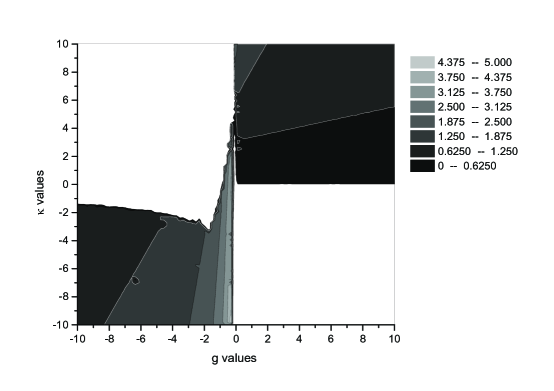
Figure 1: Contour plot showing the allowed background field amplitude value $A$, for which the localised solitary wave solution exist, here $\epsilon=0.1$.

In case of driven HNLSE, we see that $v=0$, when the equation,

$$8{\bar{\epsilon}}^{2}{\tilde{A}}^{2}k^{3}-8{\bar{\epsilon}}{\tilde{A}}k^{2}+2k-{\bar{\epsilon}}{\tilde{A}}({w}+\mu)=0,$$ (20)

is satisfied. In general, the above cubic equation can have one real, non-zero value of $k$, for appropriate equation parameters. Hence, we see that driven HNLSE has non-propagating solutions even when $k{\neq}0$, which is different from driven NLSE, since in the latter case $v=2k$.

Considering the case $k=0$, we see that, equation (12) and equation (2) have same coefficients and hence the same solutions. However, unlike the driven NLSE for this case one can have a propagating envelope with velocity

$$v=-\bar{\epsilon}\epsilon\tilde{A}.$$ (21)

Static solutions are obtained, when any one of $\tilde{A}$, $\bar{\epsilon}$ and $\epsilon$ vanish. It is interesting to note that when $\epsilon$ vanishes, as we shall show later, $\alpha$ becomes a free parameter, hence we get a static soliton of arbitrary size. The case when $\bar{\epsilon}$ vanishes, driven HNLSE simply reduces to driven NLSE, for which $k=0$ implies $v=0$. Considering the case when the third order dispersion parameter $\tilde{A}$ vanishes, one finds that for the non trivial case $\tilde{B}:\tilde{C}$ $=$ $-2:1$.

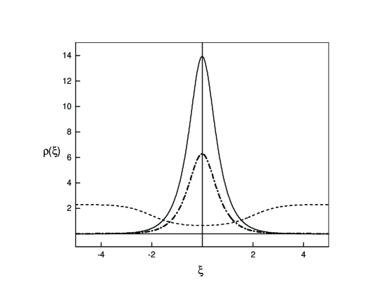
Figure 2: Density profiles of some solitons of driven NLSE.
i) Dark soliton (dashed), with $g=0.7$, $\kappa=-0.7$ and $\epsilon=-1.4$;
ii) bright soliton (solid), with $g=-0.5$, $\kappa=0.1$ and $\epsilon=-0.4$;
iii) bright soliton (dash-dotted), with $g=-0.4$, $\kappa=0.1$ and $\epsilon=-0.4$.

We now consider the case when $\epsilon=0$ for which $\omega=k^{2}-\mu$; in this case equations (4) to (7) yield,

$$q_{1}(\alpha^{4})+r_{1}\alpha^{2}+c=0.$$ (22)

Here, $q_{1}=48A^{5}g^{2}-48A^{2}g\kappa$, $r_{1}=12A^{7}g^{3}-60A^{4}g{2}\kappa+48Ag\kappa^{2}$ and $c=-18A^{6}g^{3}\kappa+9A^{3}g^{2}\kappa^{2}+9g\kappa^{3}$. Very interestingly, all of these coefficients vanish in the view of equation (4), leaving $\alpha$ as a free parameter. So, the width of the soliton, in this case, is independent of the parameter values, which means that the solitons can have arbitrary size for the given values of $g$ and $\kappa$. Similar is the case for driven HNLSE, when $\bar{\epsilon}$ vanishes from equation (12).

As noted earlier, equation (2) has singular solutions, for $D=-1$. One can show that they satisfy the relation

$$g(6{\alpha}^{2}-3\epsilon)A^{2}+\epsilon(2{\alpha}^{2}+\epsilon)+9g\kappa A-8{\alpha}^{4}=0.$$ (23)

These solutions possess one singularity in their profile, which physically corresponds to very large field intensity due to self focussing [26, 27]. When $D<-1$, singular solitons exists, with singularites existing at two different locations, between which $\sigma$ becomes negative.

4 NLSE with a generalized source

Instead of the source term of the type we have considered previously, one can have a more general one where,

$$i\frac{\partial\psi}{\partial t}+\frac{\partial^{2}\psi}{\partial x^{2}}+g\mid\psi\mid^{2}\psi+\mu\psi=\kappa e^{i(\chi(\xi)-\omega t)}.$$ (24)

Here $\chi(\xi)$ is some function. We consider the ansatz,

$$\psi(x,t)=\rho(\xi,t)e^{i(\chi(\xi)-\omega t)},$$ (25)

where $\xi=\alpha(x-vt)$. Equation (25) when substituted in equation (24) gives a complex equation in $\rho$ and $\chi$. Equating the imaginary part to zero, one gets,

$$\chi^{\prime}=\frac{v}{2\alpha}+\frac{c}{\rho^{2}}.$$ (26)

One can clearly see that the above equation suggests phase-amplitude coupling for $c{\neq}0$. We see from relation (26) an interesting case of the phase singularity of the soliton arising through phase-amplitude coupling, when $\rho$ vanishes.

Substituting this relation in the real part of equation (24), we get a non linear differential equation of the form,

$$\alpha^{2}\rho^{\prime\prime}+g\rho^{3}+\epsilon\rho=\kappa+\frac{\alpha^{2}c^{2}}{\rho^{3}},$$ (27)

where $\epsilon=(\omega+\mu+\frac{v^{2}}{4})$. The above equation can be connected with the equation governing Jacobi elliptic functions via a fractional transformation as,

$$\rho(\xi)=\frac{A+Bf(\xi|m)^{\delta}}{1+Df(\xi|m)^{\delta}},$$ (28)

where $\delta=2$ is again the maximum allowed value. This gives the consistency conditions:

$$gA^{6}+\epsilon A^{4}-(2\alpha^{2}(AD-B)(1-m)+\kappa)A^{3}=\alpha^{2}c^{2}$$ (29)

$$6A^{5}Bg+4\epsilon A^{3}B+2\epsilon A^{4}D-3\kappa A^{2}B-3\kappa A^{3}D+6\alpha^{2}(B-AD)(1-m)A^{2}B+$$

$$6\alpha^{2}(AD-B)(1-m)A^{3}D+4\alpha^{2}(2m-1)A^{3}(B-AD)=6\alpha^{2}c^{2}D$$ (30)

$$6\alpha^{2}(B-AD)(1-m)AB^{2}+18\alpha^{2}(AD-B)(1-m)A^{2}BD+$$

$$12\alpha^{2}(B-AD)(2m-1)A^{2}B+4\alpha^{2}(AD-B)(2m-1)A^{3}D+$$

$$6\alpha^{2}(AD-B)mA^{3}+15gA^{4}B^{2}+6\epsilon A^{2}B^{2}+8\epsilon A^{3}BD+\epsilon A^{4}D^{2}$$

$$-3\kappa AB^{2}-9\kappa A^{2}BD-3\kappa A^{3}D^{2}=15\alpha^{2}c^{2}D^{2}$$ (31)

$$20gA^{3}B^{3}+4\epsilon AB^{3}+12\epsilon A^{2}B^{2}D+4\epsilon A^{3}BD^{2}$$

$$-\kappa B^{3}-9\kappa AB^{2}D-9\kappa A^{2}BD^{2}-\kappa A^{3}D^{3}+$$

$$18\alpha^{2}AB^{2}D(AD-B)(1-m)-2\alpha^{2}B^{3}(AD-B)(1-m)-$$

$$12\alpha^{2}AB^{2}(AD-B)(2m-1)-2\alpha^{2}mA^{3}D(AD-B)$$

$$+12\alpha^{2}A^{2}BD(AD-B)(2m-1)=20\alpha^{2}c^{2}D^{3}$$ (32)

$$15gA^{2}B^{4}+\epsilon B^{4}+8\epsilon AB^{3}D+6\epsilon A^{2}B^{2}D^{2}$$

$$-3\kappa B^{3}D-9\kappa AB^{2}D^{2}-3\kappa A^{2}BD^{3}+6\alpha^{2}B^{3}D(AD-B)(1-m)$$

$$-4\alpha^{2}B^{3}(AD-B)(2m-1)+12\alpha^{2}AB^{2}D(AD-B)(2m-1)+$$

$$18\alpha^{2}mAB^{2}(AD-B)-6\alpha^{2}mA^{2}BD(AD-B)=15\alpha^{2}c^{2}D^{4}$$ (33)

$$6gAB^{5}+2\epsilon B^{4}D+4\epsilon AB^{3}D^{2}-3\kappa AB^{2}D^{3}$$

$$-3\kappa B^{3}D^{2}+4\alpha^{2}(B-AD)(1-2m)B^{3}D$$

$$+6\alpha^{2}m(B-AD)AB^{2}D+6\alpha^{2}m(AD-B)B^{3}=6\alpha^{2}c^{2}D^{5}$$ (34)

$$2\alpha^{2}(B-AD)mB^{3}D+gB^{6}+\epsilon B^{4}D^{2}-\kappa B^{3}D^{3}=\alpha^{2}c^{2}D^{6}$$ (35)

Since, there in total are seven simultaneous relations to fix three independent parameters, we can see that these are constrained solutions. One can also see that the phase-amplitude coupling imposes constraints on the solution space, without changing the profile of the solutions. From the above relations, one can see that $B=0$ needs $c=0$ or $D=0$. The former case has already been studied here, whereas the latter case results in a constant background solution. Here, $A{\neq}0$ requires $c{\neq}0$, hence the solutions always exist in a constant background. This should be contrasted with the case when $c=0$; for which cnoidal wave solutions are possible with $A=0$. Similarly, in $m=1$ case localised solutions with $B=0$ are allowed in the previous case, which as seen above are not found in present case. Hence, only rational solutions are possible. Moreover, we see that (29) is a sixth order polynomial, in contrast to the previous relations, this does not have analytically tractable roots leaving numerical analysis as the only tool to analyse the structure of solution space.

In conclusion, a number of interesting features have emerged from analysis of the exact solutions of the driven NLSE and HNLSE. Dark and bright solitons can exist in attractive and repulsive non-linear regimes, a feature very different for NLSE; the presence of the external source makes this possible. In a wide range of parameters, the driven HNLSE and driven NLSE have similar solutions, albeit with different sizes and velocities. Static solitons are found for both the equations. In particular, static solitons are found to have interesting properties like arbitrary scale, under certain parametric restrictions. They differ significantly for driven NLSE and HNLSE cases. In certain specific parameter regimes, solitons of arbitrary size are found. Singular solutions are also found for both the equations. The investigation of the situation, where the phase is allowed to depend upon the intensity, revealed that the corresponding solutions are highly constrained. The study of solitary waves having complex envelope, analogous to Bloch solitons in condensed matter physics, is worth investigating in the present scenario. Application of the fractional linear transformation technique employed here to other nonlinear equations is also of deep interest. Investigations along these lines are currently in progress.

References

References

- [1] Lomdahl P S and Samuelsen M R 1986 Phys. Rev. A 34, 664
- [2] Kaup D J and Newell A C 1978 Phys. Rev. B 18, 5162
- [3] Snyder A W and Love J D 1983 Optical Waveguide Theory (London: Chapman and Hall)
- [4] Malomed B A 1995 Phys. Rev. E 51, R864
- [5] Cohen G 2000 Phys. Rev. E 61, 874
- [6] Raju T S, Panigrahi P K and Porsezian K 2005 Phys. Rev. E 71, 022608
- [7] Raju T S, Panigrahi P K and Porsezian K 2005 Phys. Rev. E 72, 046612
- [8] Nozaki K and Bekki N 1983 Phys. Rev. Lett. 50, 1226
- [9] Nozaki K and Bekki N 1986 Physica D 21, 381
- [10] Das A 1989 Integrable Models (Singapore: World Scientific)
- [11] Barashenkov I V, Smirnov Yu S and Alexeeva N V 1998 Phys. Rev. E 57, 2350
- [12] Barashenkov I V, Zemlyanaya E V, and Bär M 2001 Phys. Rev. E 64, 016603
- [13] Nistazakis H E, Kevrekidis P G, Malomed B A, Frantzeskakis D J, and Bishop A R 2002 Phys. Rev. E 66, R015601
- [14] Friedland L and Shagalov A G 1998 Phys. Rev. Lett. 81, 4357
- [15] Friedland L 1998 Phys. Rev. E 58, 3865
- [16] Raju T S, Kumar C N and Panigrahi P K 2005 J. Phys. A: Math. Gen. 38, L271
- [17] Kodama Y 1985 J. Stat.Phys. 39, 597
- [18] Kodama Y and Hasegawa A 1987 J. Quantum Electron 23, 510
- [19] Hasegawa A and Kodama Y 1995 Solitons in Optical Communications (New York: Oxford University Press)
- [20] Sasa N and Satsuma J 1991 J. Phys. Soc. Jpn. 60, 409
- [21] Hirota R 1973 J. Math. Phys. 14, 805
- [22] Anderson D and Lisak M 1983 Phys. Rev. A27, 1393
- [23] Potsasek M J and Tabor M 1991 Phys. Lett. A154, 449
- [24] Palacios S L, Guinea A, Fernandez-Diaz J M and Crespo R D 1999 Phys. Rev. E60, R45
- [25] Kumar C N and Durganandini P 1999 Pramana - J.Phys. 53, 271
- [26] Mollenauer L F, Stolen R H and Gordon J P 1980 Phys. Rev. Lett. 45 1095
- [27] Fibich G and Gaeta A L 2000 Opt. Lett. 25 335