Power solution expansions of the analogue to the first Painleve equation

The fourth-order analog to the first Painlevé equation is studied. All power expansions for solutions of this equation near points $z=0$ and $z=\infty$ are found. The exponential additions to the expansion of solution near $z=\infty$ are computed. The obtained results confirm the hypothesis that the fourth-order analog of the first Painlevé equation determines new transcendental functions. By means of the methods of power geometry the basis of the plane lattice is also calculated.

1 ​​​​​​.   Introduction.

In [1] the hierarchy of the first Painlevé equation was suggested. It can be described by the relation

$$L^{n}[w]=z$$ (1.1)

where $L^{n}$ is the Lenard’s operator, which is determined by the relation [2]

$$\begin{gathered}\frac{d}{dz}L^{n+1}=L_{zzz}^{n}-4wL^{n}_{z}-2w_{z}L^{n},\,\,\quad\,\,L^{0}[w]=-\frac{1}{2}\end{gathered}$$ (1.2)

Assumed that $n=0$ in (1.2), we have $L^{1}[w]=w$. In case of $n=2$ using (1.1) we get the first Painlevé equation [3]

$$w_{zz}-3w^{2}=z$$ (1.3)

If $n=3$ in (1.1), we get the fourth-order equation [1, 2]

$$w_{zzzz}-10w\,w_{zz}-5w^{2}_{z}+10w^{3}=z$$ (1.4)

Using $n=4$, we obtain the sixth-order equation from (1.1)

$$w_{zzzzzz}-14ww_{zzzz}-28\,w_{z}\,w_{zzz}-21\,w_{zz}^{2}+70\,ww_{z}^{2}-35\,w^{4}=z$$ (1.5)

Equation (1.4) is used in describing of the waves on water [4, 5] and in the Henon-Heiles model, which characterizes the behavior of star in the middle field of galaxy [6, 7, 8].

In papers [9, 10, 11, 12, 13, 14, 15, 16, 17, 18, 19, 20, 21, 22, 23] it was shown that equation (1.4) has properties, that are typical for the Painlevé equations $P_{1}\div P_{6}$. Equation (1.4) belongs to the class of exactly solvable equations, as it has Lax pair and a lot of other typical properties of the exactly solvable equations. However it doesn’t have the first integrals in the polynomial form, that is one of the features of the Painlevé equations. Equation (1.4) seems to determine new transcendental functions just as equations $P_{1}\div P_{6}$, although the rigorous proof of the irreducibility of equation (1.4) is now the open problem.

Thereupon the study of all the asymptotic forms and power expansions of equation (1.4) is the important stage of the analysis of this equation, as this fact indirectly confirms the irreducibility of equation (1.4).

Let’s find all the power expansions for the solution of equation (1.4) in the form of

$$w(z)=c_{r}\,z^{r}+\sum_{s}\,c_{s}\,z^{s}$$ (1.6)

at $z\rightarrow\,0$, then $\omega=-1$, $s>r$ and at $z\rightarrow\,\infty$, then $\omega=1$, $s<r$.

For that we use the methods of power geometry [24, 25] by analogy with [26].

2 ​​​​​​.  The general properties of equation (1.4).

Let’s consider the fourth-order equation (1.4)

$$f(z,w)\stackrel{{\scriptstyle def}}{{=}}w_{zzzz}-10ww_{zz}-5w^{2}_{z}+10w^{3}-z=0$$ (2.1)

For monomials of equation (2.1) we have points $M_{1}=(-4,1),\,\,\,M_{2}=(-2,2),\,\,\,M_{3}=(-2,2),\,\,\,M_{4}=(0,3),\,\,\,M_{5}=(1,0)$.

The carrier of equation is defined by four points $Q_{1}=M_{1}$, $Q_{2}=M_{4}$, $Q_{3}=M_{5}$ and $Q_{4}=M_{2}=M_{3}$. Their convex hull $\Gamma$ is the triangle (fig. 1).

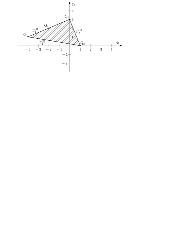
Figure 1:

This triangle has apexes $Q_{j}\,(j=1,2,3)$ and edges $\Gamma_{1}^{(1)}=[Q_{3},\,Q_{1}],\,\,\Gamma_{2}^{(1)}=[Q_{1},\,Q_{2}],\,\,\Gamma_{3}^{(1)}=[Q_{2},\,Q_{3}]$

Outward normal vectors $N_{j}\,(j=1,2,3)$ of edges $\Gamma_{j}^{(1)}\,(j=1,2,3)$ are determined by vectors

$$N_{1}=(-1,-5),\,\,\,N_{2}=(-1,2),\,\,\,N_{3}=(3,1)$$ (2.2)

The normal cones $U_{j}^{(1)}$ to edges $\Gamma_{j}^{(1)}$ are

$$U_{j}^{(1)}=\mu N_{j},\,\,\,\mu>0,\,\,\,j=1,2,3$$ (2.3)

They and the normal cones $U_{j}^{(0)}$ of apexes $\Gamma_{j}^{(0)}=Q_{j}\,\,(j=1,\,2,\,3)$ are represented at fig. 2.

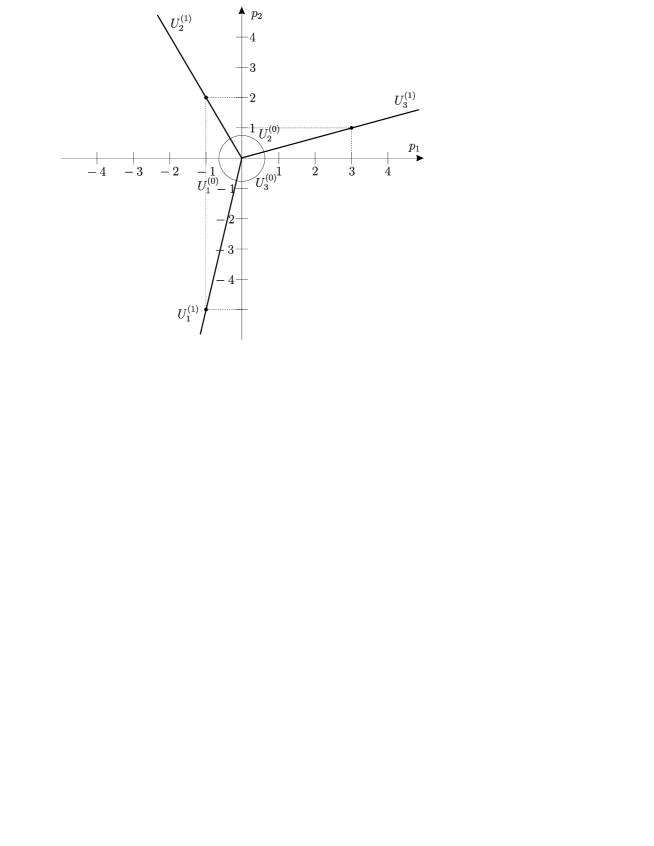
Figure 2:

If the carrier of equation (2.1) is moved by vector $-Q_{3}$, then it is situated at the lattice Z, formed by vectors

$$Q_{1}-Q_{3}=(-5,\,1),\,\,\quad\,Q_{2}-Q_{1}=(-1,\,3)$$ (2.4)

We choose the basis of the lattice as

$$B_{1}=(-5,\,1),\,\,\quad\,B_{2}=(-3,\,2)$$ (2.5)

Let’s study solutions, corresponding to the bounds $\Gamma_{j}^{(d)},\,\,d=0,1;\,\,j=1,\,2,\,3$ in view of the reduced equations, conforming to apexes $\Gamma_{j}^{(0)}(j=1,\,2,\,3)$

$$\hat{\emph{f}}_{1}^{(0)}\stackrel{{\scriptstyle def}}{{=}}w_{zzzz}=0$$ (2.6)

$$\hat{\emph{f}}_{2}^{(0)}\stackrel{{\scriptstyle def}}{{=}}10\,w^{3}=0$$ (2.7)

$$\hat{\emph{f}}_{3}^{(0)}\stackrel{{\scriptstyle def}}{{=}}\,-z=0$$ (2.8)

and reduced equations, conforming to edges $\Gamma_{j}^{(1)}(j=1,2,3)$

$$\hat{\emph{f}}_{1}^{(1)}\stackrel{{\scriptstyle def}}{{=}}w_{zzzz}-z=0$$ (2.9)

$$\hat{\emph{f}}_{2}^{(1)}\stackrel{{\scriptstyle def}}{{=}}w_{zzzz}-10\,w\,w_{zz}-5w_{z}^{2}+10w^{3}=0$$ (2.10)

$$\hat{\emph{f}}_{3}^{(1)}\stackrel{{\scriptstyle def}}{{=}}10w^{3}-z=0$$ (2.11)

Note, that the reduced equations (2.7) and (2.8) are the algebraic ones. According to [25] they don’t have non-trivial power or non-power solutions.

3 ​​​​​​.   Solutions, corresponding to apex $Q_{1}$.

Apex $Q_{1}=(-4,1)$ is corresponded to reduced equation (2.6).

Let’s find the reduced solutions

$$w=c_{r}z^{r},\,\,\,c_{r}\neq 0$$ (3.1)

for $\omega(1,r)\in U_{1}^{(0)}$.

Since $p_{1}<0$ in the cone $U_{1}^{(0)}$, then $\omega=-1,\,\,\,z\rightarrow 0$ and the expansions are the ascending power series of $z$. The dimension of the bound $d=0$, therefor

$$g(z,w)=w^{4}\,w^{-1}\,w_{zzzz}$$ (3.2)

We get the characteristic polynomial

$$\chi(r)\stackrel{{\scriptstyle def}}{{=}}g(z,z^{r})=r(r-1)(r-2)(r-3)$$ (3.3)

Its roots are

$$r_{1}=0,\,\,\,r_{2}=1,\,\,\,r_{3}=2,\,\,\,r_{3}=3$$ (3.4)

Let’s explore all these roots.

The root $r_{1}=0$ is corresponded to vector $R=(1,0)$ and vector $\omega R\in U_{1}^{(0)}$.

We obtain the family $\mathcal{F}_{1}^{(1)}\,1$ of reduced solutions $y=c_{0}$, where $c_{0}\neq 0$ is arbitrary constant and $\omega=-1$. The first variation of equation (2.6)

$$\frac{\delta\hat{\emph{f}}_{1}^{(0)}}{\delta w}=\frac{d^{4}}{dz^{4}}$$ (3.5)

gives operator

$$\mathcal{L}(z)=\frac{d^{4}}{dz^{4}}\neq 0$$ (3.6)

Its characteristic polynomial is

$$\nu(k)=z^{4-k}\mathcal{L}(z)\,z^{k}=k(k-1)(k-2)(k-3)$$ (3.7)

Equation

$$\nu(k)=0$$ (3.8)

has four roots

$$k_{1}=0,\,\,\,k_{2}=1,\,\,\,k_{3}=2,\,\,\,k_{4}=3$$ (3.9)

As long as $\omega=-1$ and $r=0$, then the cone of the problem is

$$\mathcal{K}=\{k>0\}$$ (3.10)

It contains the critical numbers $k_{2}=1,\,\,\,k_{3}=2$ and $k_{3}=3$. Expansions for the solutions, corresponding to reduced solution (3.1) can be presented in the form

$$w=c_{0}+c_{1}z+c_{2}z^{2}+c_{3}z^{3}+\sum^{\infty}_{k=4}c_{k}z^{k}$$ (3.11)

where all the coefficients are constants, $c_{0}\neq 0,\,\,\,c_{1},\,\,\,c_{2}$, $c_{3}$ are arbitrary ones and $c_{k}\,\,(k\geq 4)$ are uniquely defined. Denote this family as $\emph{G}_{1}^{(0)}1$. Expansion (3.11) with taking into account eight terms is

$$\begin{gathered}w(z)=c_{{0}}+c_{{1}}\,z+c_{{2}}\,{z}^{2}+c_{{3}}\,{z}^{3}+\left(\frac{5}{6}\,c_{{0}}c_{{2}}-{\frac{5}{12}}\,{c_{{0}}}^{3}+{\frac{5}{24}}\,{c_{{1}}}^{2}\right){z}^{4}+\\ +\left({\frac{1}{120}}\,\alpha-\frac{1}{4}\,c_{{1}}{c_{{0}}}^{2}+\frac{1}{2}\,c_{{0}}c_{{3}}+\frac{1}{3}\,c_{{1}}c_{{2}}\right){z}^{5}+\\ +\left({\frac{7}{36}}\,c_{{2}}{c_{{0}}}^{2}-{\frac{5}{36}}\,{c_{{0}}}^{4}-{\frac{1}{72}}\,c_{{0}}{c_{{1}}}^{2}+\frac{1}{9}\,{c_{{2}}}^{2}+\frac{1}{4}\,c_{{1}}c_{{3}}\right){z}^{6}+\\ +\left(\frac{1}{36}\,{c_{{1}}}^{3}+{\frac{1}{504}}\,c_{{0}}\alpha+\frac{1}{12}\,c_{{3}}{c_{{0}}}^{2}+\frac{1}{6}\,c_{{0}}c_{{1}}c_{{2}}-{\frac{5}{36}}\,c_{{1}}{c_{{0}}}^{3}+\frac{1}{6}\,c_{{2}}c_{{3}}\right){z}^{7}+...\end{gathered}$$

Let’s explore root $r_{2}=1$. The cone of the problem is $\mathcal{K}=\{k>1\}$. It contains the critical numbers $k_{2}=2,\,\,\,k_{3}=3$. The expansion of solution, corresponding to the reduced solution

$$\mathcal{F}_{1}^{(1)}2:\,\,\,w=c_{1}\,z$$

can be written as

$$w(z)=c_{1}z+c_{2}z^{2}+c_{3}z^{3}+\sum^{\infty}_{k=4}c_{k}z^{k}$$ (3.12)

where $c_{1}\neq 0,\,\,\,c_{2}$ and $c_{3}$ are the arbitrary constants. Denote this family as $\emph{G}_{1}^{(0)}2$. The expansion of solutions (3.12) with taking into account seven terms is

$$\begin{gathered}w(z)=c_{{1}}z+c_{{2}}{z}^{2}+c_{{3}}{z}^{3}+{\frac{5}{24}}\,{c_{{1}}}^{2}{z}^{4}+\left({\frac{1}{120}}\,+\frac{1}{3}\,c_{{1}}c_{{2}}\right){z}^{5}+\\ +\left(\frac{1}{4}\,c_{{1}}c_{{3}}+\frac{1}{9}\,{c_{{2}}}^{2}\right){z}^{6}+\left(\frac{1}{6}\,c_{{2}}c_{{3}}+\frac{1}{36}\,{c_{{1}}}^{3}\right){z}^{7}+...\end{gathered}$$

For root $r_{2}=2$ the cone of the problem is $\mathcal{K}=\{k>2\}$. The critical number is $k_{3}=3$. The expansion of the solutions, corresponding to the reduced solution

$$\mathcal{F}_{1}^{(1)}3:\,\,\,w=c_{2}\,z^{2}$$

takes the form

$$w=c_{2}z^{2}+c_{3}z^{3}+\sum^{\infty}_{k=4}c_{k}\,z^{k}$$ (3.13)

Denote this family as $\emph{G}_{1}^{(0)}3$. Expansion (3.13) with taking into account eight terms is

$$\begin{gathered}w(z)=c_{{2}}{z}^{2}+c_{{3}}{z}^{3}+{\frac{1}{120}}\,{z}^{5}+\frac{1}{9}\,{c_{{2}}}^{2}{z}^{6}+\frac{1}{6}\,c_{{2}}c_{{3}}{z}^{7}+\frac{1}{16}\,{c_{{3}}}^{2}{z}^{8}+\\ +{\frac{1}{1134}}\,c_{{2}}\,{z}^{9}+\left({\frac{5}{648}}\,{c_{{2}}}^{3}+{\frac{41}{60480}}\,c_{{3}}\right){z}^{10}+...\end{gathered}$$ (3.14)

For root $r_{3}=3$ the cone of the problem is $\mathcal{K}=\{k>3\}$. There is no critical number here. The expansion of solutions, corresponding to the reduced solution

$$\mathcal{F}_{1}^{(1)}4:\,\,\,w=c_{3}\,z^{3}$$

takes the form

$$w(z)=c_{3}z^{3}+\sum^{\infty}_{k=4}c_{k}\,z^{k}$$ (3.15)

Denote this family as $\emph{G}_{1}^{(0)}4$. The expansion (3.15) with taking into account four terms is

$$\begin{gathered}w(z)=c_{{3}}{z}^{3}+{\frac{1}{120}}\,{z}^{5}+\frac{1}{16}\,{c_{{3}}}^{2}{z}^{8}+{\frac{41}{60480}}\,c_{{3}}\,{z}^{10}+\ldots\end{gathered}$$ (3.16)

The expansions of solutions converge for sufficiently small $|z|$. The existence and analyticity of expansions (3.11), (3.12), (3.13) and (3.15) follow from Cauchy theorem.

4 ​​​​​​.   Solutions, corresponding to edge $\Gamma^{(1)}_{1}$.

Edge $\Gamma^{(1)}_{1}$ is conformed by the reduced equation

$$\hat{f}_{1}^{(1)}(z,y)\stackrel{{\scriptstyle def}}{{=}}y_{zzzz}-z=0$$ (4.1)

Normal cone is

$$U^{(1)}_{1}=\{-\mu(1,5),\,\,\mu>0\}$$ (4.2)

Therefor $\omega=-1$, i.e. $z\rightarrow 0$ and $r=5$. Power solutions are found in the form

$$w=c_{5}z^{5}$$

For $c_{5}$ we have

$$c_{5}=\frac{1}{120}$$ (4.3)

The only power solution is

$$\mathcal{F}_{2}^{(1)}1:\,\,\,w=\frac{z^{5}}{120}$$ (4.4)

Compute the critical numbers. The first variation of (2.9) is

$$\frac{\delta\hat{f}^{(1)}_{1}}{\delta w}=\frac{d^{4}}{dz^{4}}$$ (4.5)

We get the proper numbers

$$k_{1}=0,\,\,\,k_{2}=1,\,\,\,k_{3}=2,\,\,\,k_{4}=3$$ (4.6)

The cone of the problem

$$\mathcal{K}=\{k>5\}$$

doesn’t consist them. Solution (4.4) is corresponded to two vector indexes $\tilde{Q}_{1}=(0,1),\,\,\,\tilde{Q}_{2}=(5,0)$. There difference $B=\tilde{Q}_{1}-\tilde{Q}_{2}=(-5,\,1)$ equals to vector $Q_{1}-Q_{2}$. So solution (4.4) is conformed to lattice Z, which consists of points $Q=(q_{1},\,q_{2})=k(-3,\,2)+m(-5,\,1)=(-3k-5l,\,2k+l)$, where $k$ and $l$ are whole numbers. Points belong to line $q_{2}=-1$, if $l=-1-2k$. In this case $q_{1}=5+7k$. As long as the cone of the problem here is $\mathcal{K}=\{k>5\}$, the set of the carrier of solution expansion K takes the form

$$\textbf{K}=\{5+7n,\,\,\,n\in\mathbb{N}\}$$ (4.7)

Then the expansion of solution can be written as

$$w(z)=z^{5}\left(\frac{1}{120}+\sum^{\infty}_{m=1}c_{5+7m}\,z^{7m}\right)$$ (4.8)

Expansion (4.8) with taking into account three terms takes the form

$$w(z)=\frac{z^{5}}{120}\left(1+\frac{13\,z^{7}}{57024}+\frac{2851\,z^{14}}{79569008640}+...\right)$$ (4.9)

Equation (4.1) doesn’t have exponential additions and non-power asymptotic forms.

5 ​​​​​​.   Solutions, corresponding to edge $\Gamma^{(1)}_{2}$.

Edge $\Gamma^{(1)}_{2}$ is corresponded to the reduced equation

$$\hat{f}^{(1)}_{2}(z,w)\stackrel{{\scriptstyle def}}{{=}}w_{zzzz}-10\,w\,w_{zz}-5\,w^{2}+10\,w^{3}=0$$ (5.1)

The normal cone is

$$U^{(1)}_{2}=\{-\mu(1,-2),\,\mu>0\}$$ (5.2)

Therefor $\omega=-1$, i.e. $z\rightarrow 0$ and $r=-2$. Hence the solution of equation (5.1) we can find in the form

$$w=c_{-2}z^{-2}$$ (5.3)

For $c_{-2}$ we have the determining equation

$$c_{-2}^{2}-8\,c_{-2}+12=0$$ (5.4)

Consequently we get

$$c_{-2}^{(1)}=2,\,\,\quad\,c_{-2}^{(2)}=6$$ (5.5)

The reduced solutions are

$$\mathcal{F}_{2}^{(1)}1:\,\,\,w=2z^{-2}$$ (5.6)

$$\mathcal{F}_{2}^{(1)}2:\,\,\,w=6z^{-2}$$ (5.7)

Let’s compute the corresponding critical numbers. The first variation is

$$\frac{\delta f_{2}^{(1)}}{\delta w}=\frac{d^{4}}{dz^{4}}-10w_{zz}-10w\frac{d^{2}}{dz^{2}}-10\,w_{z}\frac{d}{dz}+30\,w^{2}$$ (5.8)

Applied to solution (5.6), it produces operator

$$\mathcal{L}^{(1)}(z)=\frac{d^{4}}{dz^{4}}-\frac{20}{z^{2}}\frac{d^{2}}{dz^{2}}+\frac{40}{z^{3}}\frac{d}{dz}$$ (5.9)

which is corresponded by the characteristic polynomial

$$\nu(k)=k^{4}-6k^{3}-9k^{2}+54k$$ (5.10)

Equation

$$\nu(k)=0$$ (5.11)

has the roots

$$k_{1}=-3,\,\,\,k_{2}=0,\,\,\,k_{3}=3,\,\,\,k_{4}=6$$ (5.12)

With reference to solution (5.7) variation (5.8) gives operator

$$\mathcal{L}^{(2)}(z)=\frac{d^{4}}{dz^{4}}+\frac{60}{z^{2}}\frac{d^{2}}{dz^{2}}-\frac{120}{z^{3}}\frac{d}{dz}+\frac{720}{z^{4}}$$ (5.13)

which is corresponded by the characteristic polynomial

$$\nu(k)=k^{4}-6k^{3}-49k^{2}+174k+720$$ (5.14)

with roots

$$k_{1}=-5,\,\,\,k_{2}=-3,\,\,\,k_{3}=6,\,\,\,k_{4}=8$$ (5.15)

The cone of the problem here is

$$\mathcal{K}=\{k>-2\}$$ (5.16)

Therefor for the reduced solution (5.6) three critical numbers belong to the cone, and there are two critical numbers for the reduced solution (5.7) in the cone of the problem.

The set of the carriers of the solution expansions K can be written as

$$\textbf{K}=\{-2+7n,\,\,\,n\in\mathbb{N}\}$$ (5.17)

Sets $\textbf{K}(0)$, $\textbf{K}(0,3)$ and $\textbf{K}(0,3,6)$ are

$$\begin{gathered}\textbf{K}(0)=\{-2+7n+2m,\,\,n,m\in\mathbb{N},\,\,n+m\geq\,0\}=\\ =\{-2,0,4,6,5,7,8,...\}\end{gathered}$$ (5.18)

$$\begin{gathered}\textbf{K}(0,3)=\{-2+7n+2m+5k,\,n,m,k\in\mathbb{N},\,\,m+n+k\geq\,0\}=\\ =\{-2,0,2,3,4,5,6,7,8,...\}\end{gathered}$$ (5.19)

$$\begin{gathered}\textbf{K}(0,3,6)=\{-2+7n+2m+5k+8l,\,n,m,k,l\in\mathbb{N},\,\,m+n+k+l\geq\,0\}=\\ =\{-2,0,2,3,4,5,6,7,8,...\}\end{gathered}$$ (5.20)

In this case the expansion for the solution of equation can be represented as

$$\begin{gathered}w(z)=\frac{2}{z^{2}}+\sum_{n,m,k,l}c_{5+7n+2m+2k+8l}\,z^{5+7n+2m+2k+8l}\end{gathered}$$ (5.21)

Denote this family as $G_{2}^{1}1$. The critical number $0$ doesn’t belong to set K, so the compatibility condition for $c_{0}$ holds automatically and $c_{0}$ is the arbitrary constant. The critical number $3$ also doesn’t belong to sets K and $\textbf{K}(0)$, therefor the compatibility condition for $c_{3}$ holds too and $c_{3}$ is the arbitrary constant. But critical number $6$ is a member of $\textbf{K}(0)$ and $\textbf{K}(0,6)$, so it is necessary to verify that the compatibility condition for $c_{6}$ holds and that $c_{6}$ is the arbitrary constant. The calculation shows that in this situation the condition holds and $c_{6}$ is the arbitrary constant too. The three-parameter power expansion of solutions, corresponding to the reduced solution (5.6) takes the form

$$\begin{gathered}w(z)=\frac{2}{{z}^{2}}+c_{{0}}-\frac{3}{2}\,{c_{{0}}}^{2}{z}^{2}+c_{{3}}{z}^{3}-\frac{5}{2}\,{c_{{0}}}^{3}{z}^{4}+\left(\frac{3}{4}\,c_{{0}}c_{{3}}-{\frac{1}{80}}\right){z}^{5}+c_{{6}}{z}^{6}-\\ -{\frac{1}{280}}\,c_{{0}}\,{z}^{7}+\left({\frac{153}{352}}\,{c_{{0}}}^{5}+{\frac{9}{44}}\,c_{{0}}c_{{6}}+{\frac{9}{176}}\,{c_{{3}}}^{2}\right){z}^{8}+\left({\frac{19}{12096}}\,{c_{{0}}}^{2}-{\frac{5}{16}}\,{c_{{0}}}^{3}c_{{3}}\right){z}^{9}+\\ +\left({\frac{25}{104}}\,{c_{{0}}}^{6}-{\frac{29}{29120}}\,c_{{3}}-{\frac{3}{26}}\,{c_{{0}}}^{2}c_{{6}}+{\frac{3}{52}}\,c_{{0}}{c_{{3}}}^{2}\right){z}^{10}+...\end{gathered}$$ (5.22)

The carrier of power expansion, corresponding to reduced solution (5.7), is formed by the sets

$$\begin{gathered}\textbf{K}(6)=\{-2+7n+8m,\,n,m\in\mathbb{N},\,\,m+n\geq\,0\}=\\ =\{-2,5,6,12,14,20,21,22,27,28,29,30,34,35,36,37,38,41,...\}\end{gathered}$$ (5.23)

$$\begin{gathered}\textbf{K}(6,8)=\{-2+7n+8m+10k,\,n,m,k\in\mathbb{N},\,\,m+n+k\geq\,0\}=\\ =\{-2,5,6,8,12,13,14,15,16,18,19,20,21,...\}\end{gathered}$$ (5.24)

The expansion for solution of equation can be written as

$$\begin{gathered}w(z)=\frac{6}{z^{2}}+\sum_{n,m,k}c_{5+7n+8m+10k}\,z^{5+7n+8m+10k}\end{gathered}$$ (5.25)

Denote this family as $G_{2}^{1}2$. The critical numbers 6 and 8 don’t belong to the set K and the number 8 doesn’t belong to the set $\textbf{K}(6)$. For numbers 6 and 8 the compatibility conditions holds automatically, therefor coefficients $c_{6}$ and $c_{8}$ are the arbitrary constants. The two-parameter expansion of solution, corresponding to the reduced solution (5.7), is

$$\begin{gathered}w(z)=\frac{6}{{z}^{2}}+{\frac{1}{240}}\,{z}^{5}+c_{{6}}{z}^{6}+c_{{8}}{z}^{8}+{\frac{29}{70502400}}\,{z}^{12}+\\ +{\frac{11}{60480}}\,c_{{6}}{z}^{13}+{\frac{25}{1292}}\,{c_{{6}}}^{2}{z}^{14}+{\frac{1}{6804}}\,c_{{8}}{z}^{15}+...\end{gathered}$$ (5.26)

According to [25], the expansions of solutions (5.22) and (5.26) don’t have power and exponential additions.

6 ​​​​​​.   Solutions, corresponding to edge $\Gamma^{(1)}_{3}$.

Edge $\Gamma^{(1)}_{3}$ is corresponded by the reduced equation

$$\hat{f}_{3}^{(1)}(z,w)\stackrel{{\scriptstyle def}}{{=}}10\,w^{3}-z=0$$ (6.1)

It has three power solutions

$$\mathcal{F}_{3}^{(1)}1:\,\,\,\,w=\varphi^{(1)}(z)=c_{1/3}^{(1)}\,z^{1/3},\,\quad\,c_{1/3}^{(1)}=\left(\frac{1}{10}\right)^{1/3}$$ (6.2)

$$\mathcal{F}_{3}^{(1)}2:\,\,\,\,w=\varphi^{(2)}(z)=c_{1/3}^{(2)}\,z^{1/3},\,\quad\,c_{1/3}^{(2)}\,=\left(\frac{1}{2}+i\sqrt{3}\right)\left(\frac{1}{10}\right)^{1/3}$$ (6.3)

$$\mathcal{F}_{3}^{(1)}3:\,\,\,\,w=\varphi^{(3)}(z)=c_{1/3}^{(3)}\,z^{1/3},\,\quad\,c_{1/3}^{(3)}\,=\left(\frac{1}{2}-i\sqrt{3}\right)\left(\frac{1}{10}\right)^{1/3}$$ (6.4)

The shifted carrier of reduced solutions (6.2) – (6.4) gives a vector

$$B=\left(\frac{1}{3},-1\right)$$ (6.5)

which equals a third of vector $Q_{2}-Q_{1}$. Therefor we explore the lattice, generated by vectors $Q_{3}-Q_{1}$ and $B$. We have $Q=(q_{1},q_{2})=k(-5,\,1)+l(-3,\,2)+m\left(\frac{1}{3},\,-1\right)=\left(2k+\frac{l}{3},\,\,k-l\right)$, where $k$, $l$ and $m$ are the whole numbers. At the line $q_{2}=-1$ we have $k+2\,l-l-m=-1$, wherefrom $m=k+2l+1$ and $q_{1}=\frac{(1+7l-14k)}{3}$. And so the carrier of solution is

$$\mathbf{K}=\left\{k=\frac{1-7n}{3},\,\,\,n\in\mathbb{N}\right\}$$ (6.6)

and the expansions of solutions take the form

$$G_{3}^{(1)}l:\,\,\,\,w=\varphi^{(l)}(z)=c^{(l)}_{1/3}z^{1/3}+\sum^{\infty}_{n=1}c^{(l)}_{(1-7n)/3}\,z^{{(1-7n)}/{3}}$$ (6.7)

Here $c^{(l)}_{1/3}$ can be found from reduced solutions (6.2) – (6.4), coefficients $c^{(l)}_{(1-7n)/3}$ are computed sequentially. The calculating of the coefficient $c_{-2}$ gives the result $c_{-2}=-\frac{1}{18}$. The expansion of solution with taking into account five terms is

$$\begin{gathered}\varphi^{(l)}(z)=c_{{1/3}}\,{z^{1/3}}-\frac{1}{18}\,{z}^{-2}-{\frac{7}{108}}\,{\frac{1}{c_{{1/3}}}}{z}^{-13/3}\,-\\ \\ -{\frac{4199}{17496}}\,{c_{{1/3}}}^{-2}\,{z}^{-{{20}/{3}}}-{\frac{28006583}{23514624}}\,{\frac{1}{{c_{{1/3}}}^{3}}}{z}^{-9}\,+...\end{gathered}$$ (6.8)

The obtained expansions seem to be divergent ones.

7 ​​​​​​.   Exponential additions of the first level.

Let’s find the exponential additions to solutions (6.2)-(6.4). We look for the solutions in the form

$$w=\varphi^{(l)}(z)+u^{(l)},\,\,\,l=1,2,3$$

The reduced equation for the addition $u^{(l)}$ is

$$M_{l}^{(1)}(z)u^{(l)}=0$$ (7.1)

where $M_{l}^{(1)}(z)$ is the first variation at the solution $w=\varphi^{(l)}(z)$. As long as

$$\frac{\delta f}{\delta w}=\frac{d^{4}}{dz^{4}}-10w_{zz}-10w\frac{d^{2}}{dz^{2}}-10w_{z}\frac{d}{dz}+30w^{2}$$ (7.2)

then

$$M_{l}^{(1)}(z)=\frac{d^{4}}{dz^{4}}-10\varphi^{(l)}_{zz}-10\varphi^{(l)}\frac{d^{2}}{dz^{2}}-10\varphi_{z}^{(l)}\frac{d}{dz}+30{\varphi^{(l)}}^{2}$$ (7.3)

Equation (7.1) takes the form

$$\begin{gathered}\frac{d^{4}u^{(l)}}{dz^{4}}-10\varphi^{(l)}_{zz}u^{(l)}-10\varphi{(l)}\frac{d^{2}u^{(l)}}{dz^{2}}-10\varphi^{(l)}_{z}\frac{du^{(l)}}{dz}+30{\varphi^{(l)}}^{2}u^{(l)}=0,\,\,\,\\ l=1,2,3\end{gathered}$$ (7.4)

Suppose that

$$\zeta^{(l)}=\frac{d\ln u^{(l)}}{dz}$$ (7.5)

then from (7.5) we have

$$\frac{du^{(l)}}{dz}=\zeta^{(l)}u^{(l)},\,\,\quad\,\frac{d^{2}u^{(l)}}{dz^{2}}=\zeta_{z}^{(l)}u^{(l)}+{\zeta^{(l)}}^{2}u^{(l)}$$

$$\frac{d^{3}u^{(l)}}{dz^{3}}=\zeta^{(l)}_{zz}u^{(l)}+3\zeta^{(l)}\zeta_{z}^{(l)}u^{(l)}+{\zeta^{(l)}}^{3}u^{(l)}$$

$$\frac{d^{4}u^{(l)}}{dz^{4}}=\zeta^{(l)}_{zzz}u^{(l)}+4\zeta^{(l)}\zeta^{(l)}_{zz}u^{(l)}+3{\zeta_{z}^{(l)}}^{2}u^{(l)}+6{\zeta^{(l)}}^{2}\zeta_{z}^{(l)}u^{(l)}+{\zeta^{(l)}}^{4}u^{(l)}$$

By substituting the derivatives

$$\frac{du^{(l)}}{dz},\,\quad\,\frac{d^{2}u^{(l)}}{dz^{2}},\,\quad\,\frac{d^{4}u^{(l)}}{dz^{4}}$$

into the equation (7.4) we get the reduced equation in the form

$$\begin{gathered}u^{(l)}\left[\zeta^{(l)}_{zzz}+4\zeta^{(l)}\zeta^{(l)}_{zz}+3{\zeta^{(l)}_{z}}^{2}+6{\zeta^{(l)}}^{2}\zeta^{(l)}_{z}+\right.\\ +\left.{\zeta^{(l)}}^{4}-10\varphi_{zz}^{(l)}-10\varphi^{(l)}\zeta^{(l)}_{z}-10\varphi^{(l)}{\zeta^{(l)}}^{2}-10\varphi_{z}^{(l)}\zeta^{(l)}+30{\varphi^{(l)}}^{2}\right]=0\end{gathered}$$ (7.6)

Let’s find the power expansions for solutions of equation (7.6). The carrier of equation (7.6) consists of points

$$\begin{gathered}Q_{1}=(-3,1),\,\,\,Q_{2}=(-2,2),\,\,\,Q_{3}=(-1,3),\\ Q_{4}=(0,4),\,\,\,Q_{5}=\left(\frac{1}{3},2\right),\,\,\,Q_{6}=\left(\frac{2}{3},0\right),Q_{7}=\left(-\frac{2}{3},1\right),\\ Q_{8}=\left(-\frac{5}{3},0\right),\,\,Q_{8+n}=\left(-\frac{5+7n}{3},0\right),\,\,Q_{9+m}=\left(-\frac{2+7m}{3},1\right),\\ Q_{10+k}=\left(\frac{1-7k}{3},2\right),\,\,Q_{11+k}=\left(\frac{12-14l}{3},0\right),\,\,\,m,n,k,l\in\mathbb{N}\end{gathered}$$ (7.7)

The closing of convex hull of points of the carrier of equation (7.6) is the strip. It is represented at fig. 3.

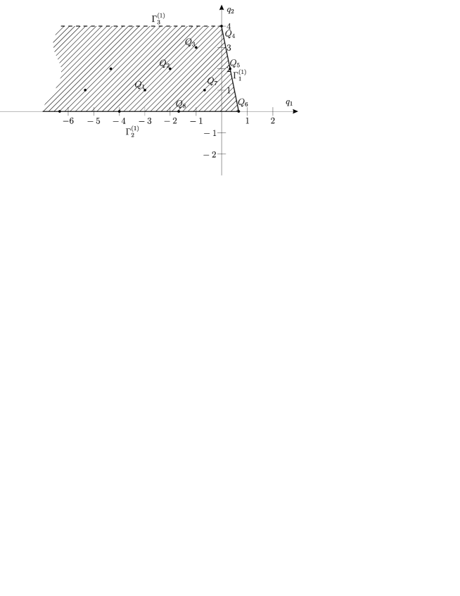
Figure 3:

The periphery of the strip contains edges $\Gamma^{(1)}_{j}\,\,(j=1,2,3)$ with normal vectors $N_{1}=(6,1),\,\,N_{2}=(0,-1),\,\,N_{3}=(0,1)$. It should take up edge $\Gamma^{(1)}_{1}$ only . This edge is corresponded by the reduced equation

$$h_{1}^{(1)}(z,\zeta)\stackrel{{\scriptstyle def}}{{=}}\zeta^{4}-10\varphi^{(l)}\zeta^{2}+30{\varphi^{(l)}}^{2}=0$$ (7.8)

Wherefrom we have

$$\zeta^{2}=\left(5+(-1)^{m-1}i\sqrt{5}\right)\varphi^{(l)},\,\,\,m=1,2$$ (7.9)

We obtain twelve solutions of equation (7.8)

$$\begin{gathered}\zeta^{(l,m,k)}=g_{1/6}^{(l,m,k)}z^{1/6},\,\,\,l=1,2,3;\,\,m,k=1,2\end{gathered}$$ (7.10)

where

$$\begin{gathered}g_{1/6}^{(1,m,k)}=\left(\frac{1}{10}\right)^{1/3}(-1)^{k-1}\left(5+(-1)^{m-1}i\sqrt{5}\right)^{1/2},\\ \,\,\,m,k=1,2\end{gathered}$$ (7.11)

$$\begin{gathered}g_{1/6}^{(2,m,k)}=\left(\frac{1}{2}+i\sqrt{3}\right)\left(\frac{1}{10}\right)^{1/3}(-1)^{k-1}\left(5+(-1)^{m-1}i\sqrt{5}\right)^{1/2},\\ \,\,\,m,k=1,2\end{gathered}$$ (7.12)

$$\begin{gathered}g_{1/6}^{(3,m,k)}=\left(\frac{1}{2}-i\sqrt{3}\right)\left(\frac{1}{10}\right)^{1/3}(-1)^{k-1}\left(5+(-1)^{m-1}i\sqrt{5}\right)^{1/2},\\ \,\,\,m,k=1,2\end{gathered}$$ (7.13)

The reduced equation is algebraic one, so it have no critical numbers. Let’s compute the carrier of the expansion for solution of equation (7.6). The shifted carrier of equation (7.6) is contained in a lattice, generated by vectors $B_{1}=\left(\frac{7}{3},0\right),\,\,B_{2}=(1,1)$. The shifted carrier of solutions (7.10) gives rise to vector $B_{3}=\left(-\frac{1}{6},1\right)$. The difference $B_{2}-B_{3}=\left(\frac{7}{6},0\right)=\frac{1}{2}B_{2}\stackrel{{\scriptstyle def}}{{=}}B_{4}$. Therefor, vectors $B_{1},B_{2}$ and $B_{3}$ generate the same lattice as vectors $B_{2},B_{4}$. Points of this lattice can be written as

$$Q=(q_{1},q_{2})=k(1,1)+m\left(\frac{7}{6},0\right)=\left(k+\frac{7m}{6},k\right)$$

At the line $q_{2}=-1$ we have $k=-1$, and so $q_{1}=-1+\frac{7m}{6}$. As long as the cone of the problem here is $\mathcal{K}=\left\{k<\frac{1}{6}\right\}$, then the set of the carriers of expansions $\mathbf{K}$ is

$$\mathbf{K}=\left\{\frac{1-7n}{6},n\in\mathbb{N}\right\}$$ (7.14)

The expansion for solution of equation (7.6) takes the form

$$\begin{gathered}\zeta^{(l,m,k)}=g^{(l,m,k)}_{1/6}z^{1/6}+\sum_{n}g^{(l,m,k)}_{(1-7n)/6}\,z^{(1-7n)/6},\,\,\,\\ l=1,2,3;\,\,\quad\,m=1,2;\,\,\quad\,k=1,2\end{gathered}$$ (7.15)

Coefficients $g_{1/6}^{(l,m,k)}$ are determined by expressions (7.11), (7.12) and (7.13). Coefficient $g^{(l,m,k)}_{-1}$ takes on a value

$$g_{-1}^{(l,m,k)}=-\frac{1}{4}\\$$ (7.16)

The expansion of solution with taking into account four terms takes the form

$$\begin{gathered}\zeta^{(l,m,k)}=g_{{1/6}}{z^{1/6}}-\frac{1}{4}\,{z}^{-1}-{\frac{7}{288}}\,\frac{\left(30\,{g_{{1/6}}}^{2}-7\,{10}^{2/3}\right)}{{g_{{1/6}}}\left(2\,{g_{{1/6}}}^{2}-{10}^{2/3}\right)}{z}^{-13/6}\,-\\ \\ -{\frac{49}{1728}}\,{\frac{30\,{g_{{1/6}}}^{4}-6\,{10}^{2/3}{g_{{1/6}}}^{2}+35\,\sqrt[3]{10}}{{g_{{1/6}}}^{2}\left(5\,\sqrt[3]{10}-2\,{10}^{2/3}\,{g_{{1/6}}}^{2}+2\,{g_{{1/6}}}^{4}\right)}}{z}^{-10/3}\,+...\end{gathered}$$ (7.17)

In view of (7.5) we can find the additions $u^{(l,m,k)}(z)$. We have

$$u^{(l,m,k)}(z)=C\exp\int\zeta^{(l,m,k)}(z)dz$$

Wherefrom we get

$$\begin{gathered}u^{(l,m,k)}(z)=C_{1}\,z^{-1/4}\,\exp\left[\frac{6}{7}\,g^{(l,m,k)}_{1/6}\,z^{7/6}+\sum^{\infty}_{n=2}\frac{6}{7(1-n)}g^{(l,m,k)}_{(1-7n)/6}z^{7(1-n)/6}\right]\\ \,\,l=1,2,3;\,\quad\,m=1,2;\,\quad\,k=1,2\end{gathered}$$ (7.18)

Here $C_{1}$ and farther $C_{2}$ and $C_{3}$ are the arbitrary constants. Addition $u^{(l,m,k)}(z)$ near $z\rightarrow\infty$ is the exponentially small one in those sectors of complex plane $z$, where

$$Re\left[g^{(l,m,k)}_{1/6}\,z^{1/6}\right]<0$$ (7.19)

Thus for three expansions $G^{(1)}_{3}l$ we get four one-parameter family of additions $G_{3}^{(1)}lG^{1}_{1}mk$, where $m=1,2$ and $k=1,2$.

8 ​​​​​​.   Exponential additions of the second level.

Let’s find exponential additions of the second level $v^{(p)}$, i.e. the additions to solutions $u^{(l,m,k)}(z)$. The reduced equation for addition $v^{(p)}$ is

$$M_{p}^{(2)}(z)v^{(p)}=0$$ (8.1)

where operator $M_{p}^{(2)}$ is the first variation of (7.6). Equation (8.5) for $v=v^{(p)}$ takes the form

$$\begin{gathered}\frac{d^{3}v}{dz^{3}}+4\zeta_{zz}v+4\zeta v_{zz}+6\zeta_{z}v_{z}+12\zeta\zeta_{z}v+\\ +6\zeta^{2}v_{z}+4\zeta^{3}v-10\varphi^{(l)}v_{z}-20\varphi^{(l)}\zeta v-10\varphi_{z}^{(l)}v=0\end{gathered}$$ (8.2)

Assumed that

$$\frac{d\ln v}{dz}=\xi$$ (8.3)

we have

$$\frac{dv}{dz}=\xi v,\,\,\quad\,\frac{d^{2}v}{dz^{2}}=\xi_{z}v+\xi^{2}v,\,\,\quad\,\frac{d^{3}v}{dz^{3}}=\xi_{zz}v+3\xi\xi_{z}v+\zeta^{3}v$$ (8.4)

From (8.2) we get equation

$$\begin{gathered}\xi_{zz}+3\,\xi\,\xi_{z}+\xi^{3}+4\zeta_{zz}+4\xi_{z}\,\zeta+4\xi^{2}\,\zeta+6\,\xi\,\zeta_{z}+12\zeta\zeta_{z}+6\,\xi\,\zeta^{2}+\\ +4\,\zeta^{3}-10\,\varphi^{(l)}\xi-20\,\zeta\,\varphi^{(l)}-10\,\varphi_{z}^{(l)}=0\end{gathered}$$ (8.5)

Monomials of equation (8.5) is corresponded by the points

$$\begin{gathered}M_{1}=(-2,1),\,\,\,M_{2}=(-1,2),\,\,\,M_{3}=(0,3),\,\,\,M_{4}=\left(-\frac{11}{6},\,0\right),\,\,\,\\ M_{5}=\left(-\frac{5}{6},1\right),\,\,\,M_{6}=\left(\frac{1}{6},2\right),\,\,\,M_{7}=\left(-\frac{5}{6},\,1\right),\,\,\,\\ M_{8}=\left(-\frac{2}{3},\,0\right),\,\,\,M_{9}=\left(\frac{1}{3},\,1\right),\,\,\,M_{10}=\left(\frac{1}{2},\,0\right),\,\,\,\\ M_{11}=\left(\frac{1}{3},1\right),\,\,\,\,M_{12}=\left(\frac{1}{2},\,0\right),\,\,\,M_{13}=\left(-\frac{2}{3},\,0\right),\,\,\,.\,.\,.\end{gathered}$$ (8.6)

The carrier of the equation (8.5) is determined by points of the set (8.6). The convex set forms the strip,which is similar to the strip, represented at fig. 3. It should examine edge $\Gamma_{1}^{(1)}$, which is passing through points

$$\begin{gathered}Q_{1}=\left(\frac{1}{2},0\right),\,\,\,Q_{2}=\left(\frac{1}{3},1\right),\,\,\,Q_{3}=\left(0,3\right)\end{gathered}$$ (8.7)

The reduced equation, corresponding to this edge, is

$$\begin{gathered}\xi^{3}+4\,\xi^{2}\,\zeta+6\,\xi\,\zeta^{2}+4\,\zeta^{3}-20\,\zeta\,\varphi^{(l)}-10\,\xi\,\varphi^{(l)}=0\end{gathered}$$ (8.8)

The basis of the lattice, corresponding to the carrier of equation (8.5) is

$$\begin{gathered}B_{1}=(1,1),\,\,\,\,B_{2}=\left(\frac{7}{6},0\right)\end{gathered}$$

The solution of equation (8.8) takes the form

$$\begin{gathered}\xi^{(l,m,k,p)}=r_{1/6}^{(l,m,k,p)}\,z^{1/6},\,\,\,\,m,k=1,2;\,\,\,\,l=1,2,3;\,\,\,\,p=1,2,3\end{gathered}$$ (8.9)

where $r=r_{1/6}^{(l,m,k,p)},\,\,\,p=1,2,3$ are the roots of the equation

$$\begin{gathered}5\,r^{3}+4\,r^{2}\,g_{1/6}^{(l,m,k)}+\left(6\,g_{1/6}^{(l,m,k)^{2}}-10\,c_{1/3}^{(l)}\right)\,r+4\,{g_{1/6}^{(l,m,k)}}^{3}\\ -20\,g_{1/6}^{(l,m,k)}\,c_{1/3}^{(l)}=0\end{gathered}$$ (8.10)

Equation (8.10) has the roots

$$\begin{gathered}r_{1/6}^{(l,m,k,1)}=-2\,g_{1/6}^{(l,m,k)},\,\quad\,r_{1/6}^{(l,m,k,2)}=-g_{1/6}^{(l,m,k)}+\left({10\,c_{1/3}^{(l)}-g_{1/6}^{(l,m,k)}}\right)^{1/2}\\ r_{1/6}^{(l,m,k,3)}=-g_{1/6}^{(l,m,k)}-\left({10\,c_{1/3}^{(l)}-g_{1/6}^{(l,m,k)}}\right)^{1/2}\end{gathered}$$ (8.11)

The set of carriers of expansions for solution $\mathbf{K}$ coincides with (7.14). The expansion of solution for $\xi^{(l,m,k,p)}$ takes the form

$$\begin{gathered}\xi^{(l,m,k,p)}=r_{1/6}^{(l,m,k,p)}z^{1/6}+\sum_{n=1}^{\infty}r^{(l,m,k,p)}_{(1-7n)/6}\,z^{(1-7n)/6},\\ \,\quad\,l=1,2,3;\,\,\quad\,m=1,2;\,\,\quad\,k=1,2;\,\quad\,p=1,2,3\end{gathered}$$ (8.12)

The computing the coefficient $r_{-1}^{(l,m,k,p)}$ gives a result $r_{-1}^{(l,m,k,p)}=1/6$. The expansion of solution with taking into account three terms is

$$\begin{gathered}\xi^{(l,m,k,p)}=r_{{1/6}}{z^{1/6}}+\frac{1}{6}\,{z}^{-1}+\left(-30\,{g_{{1/6}}}^{4}-9\,{10}^{2/3}{g_{{1/6}}}^{2}+\right.\\ +150\,{g_{{1/6}}}^{2}c_{{1/3}}-35\,c_{{1/3}}{10}^{2/3}-30\,{r_{{1/6}}}^{2}{g_{{1/6}}}^{2}+7\,{r_{{1/6}}}^{2}{10}^{2/3}-\\ -\left.60\,{g_{{1/6}}}^{3}r_{{1/6}}+6\,r_{{1/6}}g_{{1/6}}{10}^{2/3}\right)\left({10}^{2/3}-2\,{g_{{1/6}}}^{2}\right)^{-1}\\ \left(6\,{g_{{1/6}}}^{2}-10\,c_{{1/3}}+3\,{r_{{1/6}}}^{2}+8\,g_{{1/6}}r_{{1/6}}\right)^{-1}{g_{{1/6}}}^{-1}{z}^{-{\frac{13}{6}}}\end{gathered}$$ (8.13)

The exponential addition $v^{(l,m,k,p)}(z)$ to solutions $u^{(l,m,k)}(z)$ is

$$\begin{gathered}v^{(l,m,k,p)}(z)=C_{2}\,z^{1/6}\exp\left[\frac{6}{7}\,r^{(l,m,k,p)}_{1/6}\,z^{7/6}+\sum^{\infty}_{n=2}\frac{6}{7(1-n)}r^{(l,m,k,p)}_{(1-7n)/6}z^{7(1-n)/6}\right],\\ l=1,2,3;\,\quad\,m=1,2;\,\quad\,k=1,2;\,\quad\,p=1,2,3\end{gathered}$$ (8.14)

Solutions $v^{(l,m,k,p)}(z)$ seem to be divergent ones too.

9 ​​​​​​.   Exponential additions of the third level.

Let’s compute the exponential additions of the third level $y^{(s)}$, i.e. the additions to the solutions $v^{(l,m,k,p)}(z)$. The reduced equation for addition $y^{(s)}$ is

$$M_{s}^{(3)}(z)y^{(s)}=0$$ (9.1)

Operator $M_{s}^{(3)}$ is the first variation of (8.5). Equation (9.1) for $y=y^{(l,m,k,p,s)}$ takes the form

$$\begin{gathered}y_{zz}+3\xi_{z}y+3\xi y_{z}+3\xi^{2}\,y+4\,\zeta\,y_{z}+8\,\xi\,\zeta\,y+\\ +6\zeta_{z}\,y+6\zeta^{2}\,y-10\,\varphi^{(l)}\,y=0\end{gathered}$$ (9.2)

Using the substitute

$$\frac{d\ln y}{dz}=\eta$$ (9.3)

we obtain

$$\frac{dy}{dz}=\eta y,\,\,\quad\,\frac{d^{2}y}{dz^{2}}=\eta_{z}y+\eta^{2}y$$ (9.4)

From (9.4) we have equation

$$\begin{gathered}\eta_{z}+\eta^{2}+3\xi_{z}+3\xi\eta+3\xi^{2}+4\,\eta\,\zeta+8\,\xi\,\zeta+6\zeta_{z}+6\zeta^{2}-10\,\varphi^{(l)}=0\end{gathered}$$ (9.5)

Monomials of equation (9.5) is corresponded by points

$$\begin{gathered}M_{1}=(-1,\,1),\,\,\,M_{2}=(0,\,2),\,\,\,M_{3}=(-\frac{5}{6},\,0),\,\,\,M_{4}=\left(\frac{1}{6},\,1\right),\\ M_{5}=\left(\frac{1}{3},\,0\right),\,\,\,M_{6}=\left(\frac{1}{6},\,0\right),\,\,\,M_{7}=\left(\frac{1}{3},\,0\right),\,\,\,M_{8}=\left(-\frac{5}{6},\,0\right),\,\,\,\\ M_{9}=\left(\frac{1}{3},\,0\right),\,\,\,M_{10}=\left(\frac{1}{3},\,0\right),\,\,\,\,.\,.\,.\end{gathered}$$ (9.6)

The carrier of equation (9.5) is formed by points (9.6). The convex set forms the strip, which is similar to the strip, represented at fig. 3. It should examine edge $\Gamma_{1}^{(1)}$, which is passing through points

$$\begin{gathered}Q_{1}=\left(\frac{1}{3},0\right),\,\,\,Q_{2}=\left(\frac{1}{6},1\right),\,\,\,Q_{3}=\left(0,2\right)\end{gathered}$$ (9.7)

The reduced equation, corresponding to this edge, is

$$\begin{gathered}\eta^{2}+3\xi\eta+4\,\eta\,\zeta+8\,\xi\,\zeta+6\,\zeta^{2}-10\,\varphi^{(i)}=0\end{gathered}$$ (9.8)

The basis of the lattice, corresponding to the carrier of equation (9.7), is

$$\begin{gathered}B_{1}=(1,1),\,\,\,\,B_{2}=\left(\frac{7}{6},0\right)\end{gathered}$$

The solutions of equation (9.8) takes the form

$$\begin{gathered}\eta^{(l,m,k,p,s)}=q^{(l,m,k,p,s)}\,z^{1/6}\\ l=1,2,3;\,\,\,\,m,k=1,2;\,\,\,\,p=1,2,3;\,\,\,\,s=1,2;\end{gathered}$$ (9.9)

where $q^{(l,m,k,p,s)}=q$ are the roots of equation

$$\begin{gathered}q^{2}+3\,q\,r_{1/6}^{(l,m,k,p)}+4\,q\,g_{1/6}^{(l,m,k)}+8\,r_{1/6}^{(l,m,k,p)}\,g_{1/6}^{(l,m,k)}+\\ +6\,{g_{1/6}^{(l,m,k)}}^{2}-10\,c_{1/3}^{(l)}=0\end{gathered}$$ (9.10)

The roots of equation (9.10) are

$$\begin{gathered}q_{1/6}^{(l,m,k,p,s)}=-\frac{3}{2}\,r_{1/6}^{(l,m,k,p)}-2\,g_{1/6}^{(l,m,k)}+\\ +(-1)^{s-1}\,\left({\frac{9}{4}\,{r_{1/6}^{(l,m,k,p)}}^{2}-2\,{r_{1/6}^{(l,m,k,p)}}\,g_{1/6}^{(l,m,k)}-2\,{g_{1/6}^{(l,m,k)}}^{2}+10\,c_{1/3}^{(l)}}\right)^{(1/2)},\\ l=1,2,3;\,\,\,\,m,k=1,2;\,\,\,\,p=1,2,3;\,\,\,\,s=1,2;\end{gathered}$$ (9.11)

The set of carriers of expansions for solution $\mathbf{K}$ coincides with (7.14). The expansion of solution for $\eta^{(l,m,k,p,s)}$ takes the form

$$\begin{gathered}\eta^{(l,m,k,p,s)}=q^{(l,m,k,p,s)}_{1/6}z^{1/6}+\sum_{n=1}^{\infty}q^{(l,m,k,p,s)}_{(1-7n)/6}\,z^{(1-7n)/6},\,\,\,\\ l=1,2,3;\,\,\quad\,m=1,2;\,\,\quad\,k=1,2;\,\,\quad\,p=1,2,3;;\,\,\quad\,s=1,2;\end{gathered}$$ (9.12)

Coefficients $q^{(l,m,k,p,s)}_{1/6},\,\,\,s=1,2$ are determined by formulas (9.11). The computing of the coefficient $q^{(l,m,k,p,s)}_{-1}$ gives a result $q^{(l,m,k,p,s)}_{-1}=1/6$. Exponential addition $y^{(s,p,l,m,k)}(z)$ to the solutions $v^{(l,m,k,p)}(z)$ is

$$\begin{gathered}y^{(l,m,k,p,s)}(z)=C_{3}\,z^{1/6}\\ \exp\left[\frac{6}{7}\,q^{(l,m,k,p,s)}_{1/6}\,z^{7/6}+\sum^{\infty}_{n=2}\frac{6}{7(1-n)}q^{(l,m,k,p,s)}_{(1-7n)/6}z^{7(1-n)/6}\right]\\ l=1,2,3;\,\quad\,m=1,2;\,\quad\,k=1,2;\,\quad\,p=1,2,3;\,\quad\,s=1,2\end{gathered}$$ (9.13)

Thus we find three levels of the exponential additions to the expansions for solutions of equation near point $z=\infty$. Solution $w(z)$ at $z\rightarrow\infty$ with taking into account the exponential additions has the expansion

$$\begin{gathered}w(z)=c^{(l)}_{1/3}z^{1/3}-\frac{1}{18z^{2}}+\sum^{\infty}_{n=2}c^{(l)}_{(1-7n)/3}\,z^{{(1-7n)}/{3}}+\\ +C_{1}\,z^{-1/4}\,\exp\{F_{1}(z)+C_{2}\,z^{1/6}\exp\{F_{2}(z)+C_{3}\,z^{1/6}\exp\{F_{3}(z)\}\}\}\end{gathered}$$ (9.14)

where $c_{1/3}^{(l)}$ can be computed by formulas (6.2), (6.3) and (6.4); $F_{1}(z)=F_{1}^{(l,m,k)}(z)$, $F_{2}(z)=F_{2}^{(l,m,k,p)}(z)$ and $F_{3}(z)=F_{3}^{(l,m,k,p,s)}(z)$, ($l=1,2,3;\,\,\,m,k=1,2;\,\,\,p=1,2,3;\,\,\,s=1,2$) are

$$\begin{gathered}F_{1}^{(l,m,k)}(z)=\frac{6}{7}\,g^{(l,m,k)}_{1/6}\,z^{7/6}+\sum^{\infty}_{n=2}\frac{6}{7(1-n)}g^{(l,m,k)}_{(1-7n)/6}z^{7(1-n)/6}\end{gathered}$$ (9.15)

$$\begin{gathered}F_{2}^{(p,l,m,k)}(z)=\frac{6}{7}\,r^{(l,m,k,p)}_{1/6}\,z^{7/6}+\sum^{\infty}_{n=2}\frac{6}{7(1-n)}r^{(l,m,k,p)}_{(1-7n)/6}z^{7(1-n)/6}\end{gathered}$$ (9.16)

$$\begin{gathered}F_{3}^{(l,m,k,p,s)}(z)=\frac{6}{7}\,q^{(l,m,k,p,s)}_{1/6}\,z^{7/6}+\sum^{\infty}_{n=2}\frac{6}{7(1-n)}q^{(l,m,k,p,s)}_{(1-7n)/6}z^{7(1-n)/6}\end{gathered}$$ (9.17)

Coefficients $g^{(l,m,k)}_{1/6}$, $r^{(l,m,k,p)}_{1/6}$ and $q^{(l,m,k,p,s)}_{1/6}$ are defined by formulas (7.11), (7.12), (7.13), (8.11) and (9.11). The other coefficients are computed sequentially.

10 ​​​​​​.   Summary of the results and discussion.

For the solutions of fourth-order analog to the first Painlevé equation (2.1) it is obtained the following expansions.

About a point $z=0$:

1. Four-parameter (with arbitrary constants $c_{0},\,\,c_{1},\,\,c_{2}$ and $c_{3}$) family $G_{1}^{(0)}1$ of expansion for solution (3.11).

2. Three-parameter (with arbitrary constants $c_{1},\,\,c_{2}$ and $c_{3}$) family $G_{1}^{(0)}2$ of expansion (3.12).

3. Two-parameter (with arbitrary constants $c_{2}$ and $c_{3}$) family $G_{1}^{(0)}3$ of expansion (3.13).

4. One-parameter (with arbitrary constant $c_{3}$) family $G_{1}^{(0)}4$ of expansion (3.15).

Families $G_{1}^{(0)}2$, $G_{1}^{(0)}3$ and $G_{1}^{(0)}4$ are the special cases of family $G_{1}^{(0)}1$; $G_{1}^{(0)}3$ and $G_{1}^{(0)}4$ are the special cases of $G_{1}^{(0)}2$; $G_{1}^{(0)}4$ is the special case of $G_{1}^{(0)}3$.

5. Family $G_{1}^{(1)}1$ of expansion (4.8) of solution, which is the special case of families $G_{1}^{(0)}1$, $G_{1}^{(0)}2$, $G_{1}^{(0)}3$ and $G_{1}^{(0)}4$.

6. Three-parameter (with arbitrary constants $c_{0},\,\,c_{3}$ and $c_{6}$) family $G_{2}^{(1)}1$ of expansion (5.21) for solution of equation (2.1).

7. Two-parameter (with arbitrary constants $c_{6}$ and $c_{8}$) family $G_{2}^{(1)}2$ of expansion (5.25) for solution of equation (2.1).

All listed expansions converge for sufficiently small $|z|$.

About a point $z=\infty$:

8. Three expansions $G_{3}^{(1)}l\,\,(l=1,2,3)$, described by formulas (6.2), (6.3) and (6.4). For each of these expansions it is found four exponential additions $G_{3}^{(1)}lG_{1}^{1}mk\,\,(m,k=1,2)$ expressed by formula (7.18). For them it is also computed exponential additions $G_{3}^{(1)}lG_{1}^{1}mkG_{1}^{(1)}p\,\,(m,k=1,2;p=1,2,3)$, and then the proper differential additions $G_{3}^{(1)}lG_{1}^{(1)}mkG_{1}^{(1)}pG_{1}^{(1)}s\,\,(m,k=1,2;p=1,2,3;s=1,2)$ are found too.

The existence and analyticity of expansions, described in items 1-7, follow from Cauchy theorem. Families $G_{2}^{(1)}l\,\,$ and $G_{2}^{(1)}2$ were first found in the paper [13]. However the structure of expansions $G_{2}^{(1)}1$ and $G_{2}^{(2)}2$ was not discussed earlier. The other families of expansions of solution are found for the first time.

Comparing the power expansions of equation (2.1) with power expansions of Painlevé equations $P_{1}\div P_{6}$ [26, 27, 28, 29, 30, 31, 32, 33, Bruno11, Bruno12, 34] we note, that they differ. This fact can be interpreted as the additional case for the hypothesis, that the fourth-order equation (2.1) determines new transcendental functions just as equations $P_{1}\div P_{6}$.

11 ​​​​​​.   Appendix. The computation of the basis of the plane lattice.

Let there is a set $\mathbf{S}$ of points $Q_{1},\,\,...,\,\,Q_{m}$ on the plane $\mathbb{R}^{2}$, and there is a zero among them. Our aim is to compute the basis $B_{1},\,\,B_{2}$ of the minimal lattice $\mathbf{Z}$, which contains all the points of set $\mathbf{S}$. The minimality of lattice $\mathbf{Z}$ means that there is no other lattice $\mathbf{Z}\subset\mathbf{Z}$ and $\mathbf{Z}_{1}\neq\mathbf{Z}$, which also contains set $\mathbf{S}$. The computation is divided into three steps.

Step 1. Let $Q_{m}=0$, and the others $Q_{j}\neq 0$. For all pairs of vectors $Q_{j},\,\,Q_{k},\,\,1\leq j,\,k<m,j\neq k$ compose the determinants

$$\det(Q_{j}Q_{k})\stackrel{{\scriptstyle def}}{{=}}\Delta_{jk}.$$ (11.1)

Among pairs with $\Delta_{jk}\neq 0$ we find one with $|\Delta_{jk}|=\min|\Delta_{jk}|\neq 0$ in all $j,k=1,\,\,...,\,\,m-1$. If there are few such pairs, we can take any of them. Suppose for the sake of simplicity that it is pair $Q_{1},\,\,Q_{2}$. Other pairs $Q_{3},\,\,...,\,\,Q_{m-1}$ are arbitrary ordered.

Step 2. Let’s find the basis of the lattice, generated by vectors $Q_{1},Q_{2},Q_{3}$. Let $Q_{3}=aQ_{1}+bQ_{2}$, where $a$ and $b$ are the rational quantities. Denote integer part of number $a\in\mathbb{R}$ as $[a]$ and the fractional part as $\{a\}$, i.e. $\{a\}=a-[a]$. Denote $Q^{\prime}_{3}=\{a\}Q_{1}+\{b\}Q_{2}$. Suppose that $\min|\det(Q^{\prime}_{3}Q_{i})|$ for $i=1,2$ reaches at $i=1$. Then we take $Q_{1}$ and $Q^{\prime}_{3}$ as the basis vectors and use them to express $Q_{2}$, i.e. we get $Q_{2}=a_{1}Q_{1}+bQ^{\prime}_{3}$. Replace vector $Q_{2}$ by $Q^{\prime}_{2}=\{a_{1}\}Q_{1}+\{b_{1}\}Q^{\prime}_{3}$. Among three vectors $Q_{1},Q^{\prime}_{2},Q^{\prime}_{3}$ we find the pair with the least modulus of determinant. Using this pair we distribute the third vector, take his fractional part and so on. At some step $l$ we obtain that the fractional part of the third vector equals zero. The latest pair of vectors $Q^{(l)}_{2},\,\,Q^{(l)}_{3}$ gives the basis of minimal lattice, containing the points $Q_{1},\,\,Q_{2},\,\,Q_{3}$.

Step 3. For vectors $Q^{(l)}_{2},\,\,Q^{(l)}_{3},\,\,Q_{4}$ we realize step 2 and get vectors $\tilde{Q}_{3},\,\tilde{Q}_{4}$ and so on. After looking through all $Q_{j},\,\,j\leq m-1$, we get the pair of vectors $Q^{*}_{m-2},\,\,Q^{*}_{m-1}$, which is the basis of minimal lattice, containing the set $\mathbf{S}$.

Remark. The analogous algorithm allows as to find the basis of minimal lattice in $\mathbb{R}^{n}$, containing the given finite set $\mathbf{S}$. If $n=1$ it’s the Euclid algorithm.

Example 8.1. Let’s consider equation (1.4). It’s carrier consists of six points (2.1). Move them by vector $Q_{4}=(1,0)$. We obtain

$$Q^{\prime}_{1}=(-5,\,\,1),\,\,\,Q^{\prime}_{2}=(-3,\,\,2),\,\,\,Q^{\prime}_{3}=(-1,\,\,3),\,\,\,Q^{\prime}_{4}=0$$

For vectors $Q^{\prime}_{1},\,\,Q^{\prime}_{2},\,\,Q^{\prime}_{3}$ we compute the pairwise determinants

$$\Delta_{12}=\left|\begin{gathered}-5\,\,\,1\\ -3\,\,\,2\end{gathered}\right|=-7,\,\,\,\,\Delta_{13}\left|\begin{gathered}-5\,\,\,1\\ -1\,\,\,3\end{gathered}\right|=-14,\,\,\,\,\Delta_{23}\left|\begin{gathered}-3\,\,\,2\\ -1\,\,\,3\end{gathered}\right|=-7.$$ (11.2)

Thus as the initial pair we can use vectors $Q^{\prime}_{1},\,\,Q^{\prime}_{2}$ or $Q^{\prime}_{2},\,\,Q^{\prime}_{3}$. Let’s take $Q^{\prime}_{1},\,\,Q^{\prime}_{2}$ to fix the idea. We look for the expansion $Q^{\prime}_{3}=aQ^{\prime}_{1}+bQ^{\prime}_{2}=a(-5,1)+b(-3,2)$, for that we are to solve the linear system of equations

$$\begin{gathered}-5a-3b=-1,\\ a+2b=3.\end{gathered}$$ (11.3)

We get $a=-1,\,\,b=2$. As long as $\{a\}=\{b\}=0$, then the vectors $B_{1}=Q^{\prime}_{1}$ and $B_{2}=Q^{\prime}_{2}$ generate the basis of the lattice of shifted carrier of equation (1.4).

References

- [1] Kudryashov N.A. The first and second Painlevé equations of higher order and some relations between them // Phys. Letters. A. 1997. V. 224. N 6. P. 353–360.
- [2] Kudryashov N.A. Analitical theory of nonlinear differential equations, Moscow – Igevsk, Institute of Computer research, 2004. 360 p.
- [3] Golubev V.V. Lectures on integration of the equation of motion of a rigid body about a fixed point, Moscow, Gostekhizdat, 1953. 288 p. (in Russian).
- [4] Olver P.J. Hamilton and non-Hamilton models for water waves // Lecture Notes in Physics. N.Y.: Springer, 1984. N 195. P. 273-290.
- [5] Kudryashov N.A. First integrals of nonlinear wave dynamics // Applied Mathematics and Mechanics, 2005. v. 69. No. 2. pp. 884-894 (in Russian).
- [6] Hénon M., Heiles C. The applicability of the third integral of motion: some numerical experiments // Astron. J. 1964. V. 69. N 1. P. 73–79.
- [7] Fordy A.P. The Hénon — Heiles system revisited // Physica D. 1991. V. 52. N 2–3. P. 204–210.
- [8] Hone Andrew N.W. Non – autonomous Hénon — Heiles system // Physica D. 1998. V. 118 P. 1 – 16.
- [9] Kudryashov N.A. On new transcendents defined by nonlinear ordinary differential equations // J. Phys. A.: Math. Gen. 1998. V. 31. N 6. P. L.129–L.137.
- [10] Kudryashov N.A. Transcendents defined by nonlinear fourth-order ordinary differential equations // J. Phys. A.: Math. Gen. 1999. V. 32. N 6. P. 999–1013.
- [11] Kudryashov N.A. Fourth-order analogies to the Painlevé equations // J. Phys. A.: Math. Gen. 2002. V. 35. N 21. P. 4617–4632.
- [12] Kudryashov N.A. Amalgamations of the Painlevé equations // J. Math. Phys., 2003, V. 44. N 12. P. 6160–6178
- [13] Kudryashov N.A., Soukharev M.B. Uniformization and Transendence of solutions for the first and second Painleve hierarchies, Physics Letters A v. 237, 1998, 206-216
- [14] Kudryashov N.A., Soukharev M.B. Discrete equations corresponding to fourth - order differential equations of the P2 and K2 hierarchies, ANZIAM, Industrial and Applied Mathematics, 2002
- [15] Kudryashov N.A. Nonlinear differentil equations of the fourth order with solutions in the form of transcendents, Theoretical and mathematical physics, v. 122, No. 1, 2000, 72 - 86 (in Russian)
- [16] Kudryashov N.A., Pickering A. Rational solutions for Schwarzian integrable hierarchies, Journal of Physics A, Math. Gen., v. 31, 1998, 999 - 1014
- [17] Creswell G., Joshi N. The discrete first,second and thirty - fourth Painleve hierarchies, Journal of Physics A, Math. Gen., v. 32, 1999, 655 - 669
- [18] Mugan U., Jrad F. Painleve test and the first Painleve hierarchy, Journal of Physics A, Math. Gen., v. 32, 1999, 7933 - 7952
- [19] Cosgrove C.M. Higher - order Painleve equations in the polynomial class. I. Bureau symbol P2, Study Appl. Math., v. 104, 2000, 1- 65
- [20] Gordoa P.R. Backlund transformations for the second member of the first Painleve hierarchy, Physics Letters A, v. 287, 2001, 365 - 370
- [21] Pickering A. Coalescence limits for higher order Painleve equations, Physics Letters A, v. 301, 2002, 275 - 280
- [22] Clarkson P.A., Hone A.N.W., Joschi N. Hierarchies of difference equations and Backlund transformations, Journal of Nonlinear Mathematical physics, v. 10, 2003
- [23] Kawai T., Koike T., Nishikawa Y., Takei Y. On the complete description of the Stokes geometry for the first painleve hierarchy, 2004, preprint/RS/RIMS 1471, Kioto
- [24] Bruno A.D. Power geometry in algebraic and differential equations, Moscow, Nauka, Fizmatlit, 1998, 288 p. (in Russian).
- [25] Bruno A.D. Asimptotics and expansions of solutions for ordinary differential equation, Uspekhi of Mathematical sciences, v.59, No. 3, 2004, pp. 31-80 (in Russian).
- [26] Bruno A.D., Petrovich V.Yu. Particularities of solutions of the first Paileve equation, Moscov, Preprint Keldysh Institute of Applied Mathematics, No.75, 2004,(in Russian).
- [27] Bruno A.D. Power Geometry as a new calculus, in book H.G.W. Begehr et al (eds) Analysis and Applications, ISAAC, 2001, 51-71, 2003 Kluwer
- [28] Bruno A.D., Chukhareva I.B. Power expansions of the sixth Painleve equation, Moscow, Preprint Keldysh Institute of Applied Mathematics, No.49, 2003 (in Russian).
- [29] Bruno A.D., Karulina E.S. Power expansions of the fifth Painleve equation, Moscow, Preprint Keldysh Institute of Applied Mathematics, No. 50, 2003.
- [30] Bruno A.D., Zavgorodnaya Yu.V. Power series and non – power asimptotics of the second Painleve equation, Moscow, Preprint Keldysh Institute of Applied Mathematics, No. 48, 2003.
- [31] Bruno A.D., Gridnev A.V. Power and exponential expansions of the third Painleve equation, Moscow, Preprint Keldysh Institute of Applied Mathematics, No. 51, 2003.
- [32] Bruno A.D., Karulina E.S. Power expansions of the fifth Painleve equation, Reports of Russian Academy Sciences, 2004, v. 395, No. 4, pp. 439-444.
- [33] Bruno A.D., Goruchkina I.B. Power expansions of the sixth Painleve equation,Reports of Russian Academy Sciences, v. 395, 2004, No. 6, pp. 733-737.
- [34] Gromak V.I., Laine I., Shimomura S. Painleve Differential Equations in the Complex Plane, Walter de Gruyter, Berlin, New York, 2002.