Discrete soliton mobility in two-dimensional waveguide arrays with saturable nonlinearity

Abstract

We address the issue of mobility of localized modes in two-dimensional nonlinear Schrödinger lattices with saturable nonlinearity. This describes e.g. discrete spatial solitons in a tight-binding approximation of two-dimensional optical waveguide arrays made from photorefractive crystals. We discuss numerically obtained exact stationary solutions and their stability, focussing on three different solution families with peaks at one, two, and four neighboring sites, respectively. When varying the power, there is a repeated exchange of stability between these three solutions, with symmetry-broken families of connecting intermediate stationary solutions appearing at the bifurcation points. When the nonlinearity parameter is not too large, we observe good mobility, and a well defined Peierls-Nabarro barrier measuring the minimum energy necessary for rendering a stable stationary solution mobile.

I Introduction

There is a large current interest in nonlinear mechanisms for storage and transport of localized coherent packages of energy in spatially periodic systems, which may be described by discrete lattice models in one, two, or three spatial dimensions. Such systems quite generally may support intrinsic localized modes, or discrete breathers, which are exact, generally time-periodic, spatially localized solutions to the underlying dynamical lattice equations and, under certain conditions, also may show mobility. For a recent review of properties and applications of such intrinsic localized modes, see CFK04 . In particular, within nonlinear optics such localized modes may appear as discrete spatial solitons in periodic structures describing arrays of coupled waveguides. See, e.g., SKES03 ; CLS03 for reviews of experimental observations as well as theoretical modelling of discrete spatial solitons, and Chen05 ; Matuszewski and references therein for more recent experimental results.

In such systems, the longitudinal variable along the waveguides plays the role of time in the dynamical lattice equations, while the arrays themselves may be either one-dimensional (1D) (e.g. Eisenberg ; Fleischer1D ; NOKK03 ) or two-dimensional (2D) (e.g. Fleischer2D ) transversally.

Traditionally CJ88 ; Eisenberg , most attention has been put on waveguide arrays constructed from Kerr nonlinear media, in which case the appropriate lattice model derived from coupled-mode theory (tight-binding type approximation) is the cubic discrete nonlinear Schrödinger (DNLS) equation (see, e.g., EJ03 for a review on properties and applications of this model). However, more recently (e.g. Fleischer1D ; NOKK03 ; Fleischer2D ; Chen05 ; Matuszewski and references therein) much experimental effort has been devoted to generating discrete solitons in photorefractive media, where the nonlinearity is not anymore of pure Kerr type Efremidis . In particular, optically-induced lattices with focusing as well as defocusing nonlinearities were created e.g. in Fleischer1D ; NOKK03 ; Fleischer2D , leading to direct observation of many earlier predicted phenomena such as spatial gap solitons Fleischer1D and solutions of different symmetries (odd and even) in 1D arrays NOKK03 . In addition, the recent works Chen05 ; Matuszewski have reported observation of spatial gap solitons and self-trapping also in 1D permanent waveguide arrays with photovoltaic defocusing nonlinearity, showing strong saturation at higher powers. In this case, the appropriate lattice model in the tight-binding limit is a 1D DNLS equation with saturable on-site nonlinearity (a discrete version of the Vinetskii-Kukhtarev Vinetskii equation), which was introduced in Stepic04 and further studied in HMSK04 ; Khare04 ; Maluckov05 ; CE05 . It is important to remark, that the discrete model used in Maluckov05 to model waveguide arrays with photovoltaic defocusing nonlinearity is mathematically equivalent CE05 to the model for focusing nonlinearity of Stepic04 ; HMSK04 . A recent discussion and experimental demonstration of this equivalence was given in Matuszewski .

One remarkable property of the 1D saturable DNLS equation, discovered in HMSK04 , is the boundedness, and at certain points even vanishing, of the so-called Peierls-Nabarro (PN) potential barrier as a function of the soliton power. The PN barrier for DNLS-like equations may be defined KC93 as the difference in energy (Hamiltonian) between the two fundamental localized modes centered at respectively in-between lattice sites, at the same power (norm) (the latter being a conserved quantity for the dynamics). Thus, it is expected to give a lower bound to the amount of additional energy necessary to render a stable stationary solution mobile. It was also numerically confirmed HMSK04 ; Maluckov05 ; CE05 that the mobility of high-power localized solutions in the saturable 1D DNLS model was considerably enhanced compared to the cubic DNLS model, where the PN-barrier grows rapidly as the power increases pnpMor . Another peculiar property of the 1D saturable DNLS model is the existence of a family of exact analytical sech-shaped solutions, centered at arbitrary lattice positions, for some particular regimes of parameter values Khare04 . The power of these solutions, which are linearly marginally stable, depends continuously on the position of their center, and it can be shown that this solution family exists in a neighborhood of the first zero of the PN barrier, bifurcating with the site-centered and bond-centered solution families exactly at the points where these families exchange their stability. Thus, the analytical solutions constitute a family of ‘intermediate’ symmetry-broken solutions connecting site-centered and bond-centered solutions, analogously to the scenario for enhanced mobility described for another type of extended 1D DNLS equation in OJE03 , as well as for more general chains of coupled oscillators in Cretegny98 .

However, for 2D arrays, much less is known about discrete soliton mobility. Essentially, as was described in Christiansen96 , for cubic nonlinearity only wide discrete solitons are mobile. However, these are unstable to a ‘quasicollapse’ process, so that after moving a few lattice sites the broad solitons self-focus into narrow localized peaks, which get pinned by the lattice Christiansen96 . It is our purpose here, to show that a saturable nonlinearity may, under certain conditions, lead to highly mobile discrete solitons also for 2D waveguide arrays. The study of discrete soliton mobility has been suggested to be one of the most important issues in the implementation of these theoretical concepts in all-optical switching schemes for one-dimensional nonlinear arrays rodrigo and very recently for two-dimensional ones in a ‘reduced’ geometry reduced . For this reason, the two-dimensionality can be viewed as a large improvement in this direction, because of the promising possibility of multiple-site connections and the direct integration with photonic crystals.

An interesting analogy may be drawn to what is known within the field of polarons, where in the case of the standard semiclassical Holstein model with harmonic on-site oscillator potentials the stable (small) polarons are always pinned to the lattice in 2D, while if a realistic saturable anharmonicity is taken into account for the oscillator potentials, moving polarons may also exist ZCR98 . In the former case, the static polarons are obtained as stationary solutions to the cubic DNLS equation, while in the latter case as solutions to the saturable DNLS equation (although the dynamics of the polarons is more complex as it involves electron as well as phonon degrees of freedom).

The structure of this paper is as follows. In Sec. II we describe the 2D saturable DNLS equation, its basic properties, and the region of existence for localized solutions. Next, in Sec. III we analyze the stability of these solutions and we introduce the concept of Intermediate Solutions. In Sec. IV, we present our results for the mobility of localized solutions in 2D arrays. Finally, Sec. V concludes the paper.

II Model

We consider the following (general) form of the 2D saturable DNLS equation for an isotropic medium, analogous to the 1D model in Stepic04 ; HMSK04 ; CE05 ,

$$i\frac{\partial u_{n,m}}{\partial\xi}+\Delta u_{n,m}-\gamma\frac{u_{n,m}}{\left(1+|u_{n,m}|^{2}\right)}=0,$$ (1)

where $\xi$ is the normalized propagation distance, $u_{n,m}$ describes the electric field amplitude in the $\{n,m\}$ site, $\Delta$ represents the 2D discrete Laplacian, $\Delta u_{n,m}\equiv u_{n+1,m}+u_{n-1,m}+u_{n,m+1}+u_{n,m-1}$. The parameter $\gamma$ is given by the ratio between the nonlinear parameter and the coupling constant Stepic04 ; HMSK04 ; CE05 . We choose $\gamma>0$ in our computations without loss of generality. Note that, although this implies that we are formally restricting to a focusing nonlinearity, our results are immediately translated to the defocusing case through the staggering transformation $u_{n,m}\rightarrow(-1)^{m+n}u_{n,m},\xi\rightarrow-\xi$. We use an isotropic approximation which essentially considers the coupling between neighboring sites in the $\hat{n}$ and $\hat{m}$ directions as equal. In the experiment, the intrinsic anisotropy of photorefractive materials can be reduced by changing the lattice orientation relative to the crystal axis iso . The two conserved quantities for (1) are the energy (Hamiltonian)

$$H=-\sum_{n,m=1}^{N,M}\left[(u_{n+1,m}+u_{n,m+1})\ u_{n,m}^{*}\right.$$

$$\left.-\frac{\gamma}{2}\ln(1+|u_{n,m}|^{2})+c.c.\right],$$ (2)

and the Power (norm)

$$P=\sum_{n,m=1}^{N,M}|u_{n,m}|^{2}.$$ (3)

Thus, for small $P$, Eq. (1) reduces to the cubic DNLS equation with focusing nonlinearity of strength $\gamma$, which then may be replaced by unity through rescalings, while for larger $P$ saturation effects become important and $\gamma$ is left as an independent parameter. Note that slightly different forms of the saturable DNLS equation were considered (in 1D) in Khare04 ; Maluckov05 , but these are easily shown to be equivalent to the model of Stepic04 ; HMSK04 ; CE05 through simple rescalings and gauge transformations CE05 . In Stepic04 ; HMSK04 ; Maluckov05 the authors study analytically the case of $\gamma\approx 9$, based on experimental parameters. We decided to study, for the two-dimensional array, a similar case for $\gamma=10$. As it further will be explained, we also study the case of $\gamma=4$ where we found that a good mobility can be observed for lower level of power ($P$).

To study the dynamics we introduce a definition of the soliton center in the direction $\hat{n}$ (horizontal direction) as a function of $\xi$,

$$<n>\left(\xi\right)\equiv\sum_{n,m=1}^{N,M}n\ |u_{n,m}(\xi)|^{2}/\sum_{n,m=1}^{N,M}|u_{n,m}(\xi)|^{2},$$ (4)

with an equivalent definition in the vertical direction $\hat{m}$ for $<m>(\xi)$. We define “axial propagation” as the propagation in the $\hat{n}$ ($k_{x}\neq 0,k_{y}=0$) or in the $\hat{m}$ ($k_{y}\neq 0,k_{x}=0$) directions, and “diagonal propagation” when we launch the solution with the same angle in both directions ($k_{x}=k_{y}\neq 0$).

Stationary solutions to (1) are those of the form $u_{n,m}(\xi)=u_{n,m}e^{i\lambda\xi}$, where $\lambda$ represents the spatial frequency in the propagation direction. As we will mainly consider the fundamental localized solutions, we will assume $u_{n,m}$ to be real (although stationary localized solutions with nontrivial complex $u_{n,m}$, such as vortex solitons, generally also exist in 2D photorefractive optical lattices Yang ). Using a Newton-Raphson method, we have found the same types of stationary solutions as described, e.g., in Ref. 2Dkevre for the 2D cubic model. Using the usual optical terminology Eisenberg , we rename these solutions: one-peak solutions, as Odd-Odd (OO) (Fig. 1(a)); two-peaks solutions, as Odd-Even (OE) (Fig. 1(b)); four-peaks solutions, as Even-Even (EE) (Fig. 1(c)).

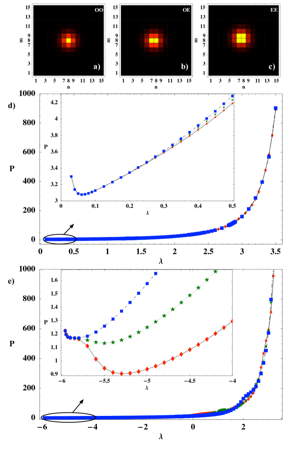
Figure 1: (Color online). (a) OO profile. (b) OE profile. (c) EE profile. (d) and (e) $P$ versus $\lambda$ for $\gamma=4$ and for $\gamma=10$, respectively. Diamonds, stars, and squares represent OO, OE, and EE solutions, respectively. System size $N=M=15$ ((d) and (e) insets: $N=M=31$).

The region of existence (see Fig. 1) of localized solutions in this system has a very different structure compared to the cubic DNLS case Mez ; 2Dkevre . This can be understood by considering the properties of plane wave-solutions to Eq. (1) in the limits of small and large amplitudes, respectively. For small-amplitude plane waves, it is easy to show, by neglecting the term $|u_{n,m}|^{2}$ in the denominator of the last term in Eq. (1), that the linear band corresponds to $\{-\gamma-4,-\gamma+4\}$; the superior limit ($\lambda=0$ for $\gamma=4$ and $\lambda=-6$ for $\gamma=10$, see Fig. 1) corresponding to constant-amplitude solutions (zero wave vector) and being the border where small-amplitude delocalized and localized solutions are connected. On the other hand, in the high-amplitude limit, we may completely neglect the last term in Eq. (1) due to the saturable nature of the nonlinearity, and thus in this limit plane waves constitute the band $-4\leq\lambda\leq 4$ (independent of $\gamma$); again with the superior limit $\lambda=4$ corresponding to the constant-amplitude (zero wave vector) solution. The superior limit for localized solutions is observed to be $\lambda=4$ by increasing the frequency (see Fig. 1), and thus the region of existence for localized modes is between the low-amplitude and high-amplitude limits for the upper band edge (zero wave vector) plane wave.

Note that, similarly to the cubic 2D DNLS equation Mez ; Christiansen96 ; Flach ; 2Dkevre , the power for the localized solutions is non-zero in the small-amplitude limit, and, when the frequency increases, the power first decreases until it reaches a minimum. When the frequency of the localized solutions increases further, the power increases indefinitely. However, the nonlinearity is saturable, which means that there is some threshold value for the amplitudes beyond which localization effects should diminish. For instance, if we take an OO solution (Fig. 1(a)), we can see that when the central site achieves such an amplitude threshold value, the surrounding sites begin to increase their amplitudes, delocalizing the profile and evolving to a high-amplitude plane wave. An analogous scenario was discussed, in a polaron context, in Ref. ZCR98 , and similar properties can also be described for the 1D saturable problem Stepic04 ; HMSK04 ; Maluckov05 .

III Stability analysis of two-dimensional localized solutions

Linear stability of stationary solutions may be investigated in a standard way (see, e.g., Ref. CE85 ) by writing $u_{n,m}(\xi)=(u_{n,m}+\phi_{n,m}(\xi))e^{i\lambda\xi}$, leading to the linearized equation for $\phi_{n,m}$, the perturbation function (PF). To solve this problem numerically, we use the technique outlined in Ref. Khare04 for the stability analysis of localized solutions in a similar nonlinear discrete medium. We split the PF into real and imaginary parts, $\phi_{n,m}=x_{n,m}+iy_{n,m}$ ($x,y\in\Re$), and insert them into the linearized equation. Taking a two-dimensional square discrete array ($N=M$) to compute stationary solutions and to perform their stability analysis, we proceed to map the 2D problem to a 1D representation. Defining $\overrightarrow{Z}$ as the vector ${Z_{1},...,Z_{N^{2}}}$ ($Z=X+iY$), we can write the equations for the perturbation functions in a one-dimensional representation as

$$\dot{\overrightarrow{X}}+\mathbf{A}\overrightarrow{Y}=0\ \text{and}\ \dot{\overrightarrow{Y}}-\mathbf{B}\overrightarrow{X}=0\Rightarrow$$

$$\ddot{\overrightarrow{X}}+\mathbf{AB}\overrightarrow{X}=0\ \text{and}\ \ddot{\overrightarrow{Y}}+\mathbf{BA}\overrightarrow{Y}=0,$$ (5)

where $\mathbf{A}$ and $\mathbf{B}$ are $N^{2}\times N^{2}$ matrices, depending of the $u_{n,m}$ profiles. Now, the stability analysis consists in finding the eigenvalues of the matrix $\mathbf{AB}$ (the matrix $\mathbf{BA}$ has the same eigenvalues Khare04 ). If all the eigenvalues are positive the solutions of the problem (PF’s) are oscillatory functions, which implies stability. On the other hand, a negative or complex eigenvalue means the existence of exponentially increasing PF’s, implying instability.

For a given frequency $\lambda$ we compute the Power $P$, the Hamiltonian $H$, and the $\mathbf{AB}$ eigenvalues for the OO, OE, and EE solutions.

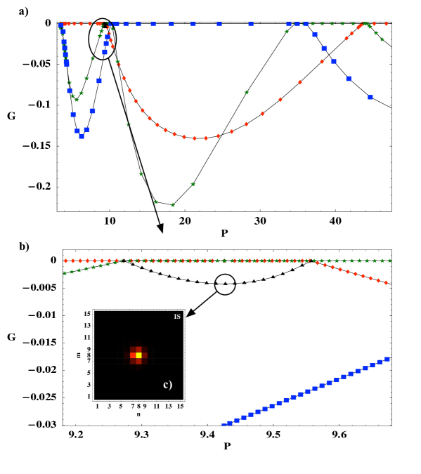
Figure 2: (Color online). Results for $\gamma=4$. (a) Smallest eigenvalue $G$ versus Power. (b) Zoom of (a) in the region $P\sim 9.4$. (c) Profile of intermediate solution (IS). Diamonds, stars, squares, and triangles represent OO, OE, EE, and IS solutions, respectively.

We take the most negative eigenvalue of each solution, calling it “$G$”, and we plot it for different powers in Fig. 2(a) and (b) for $\gamma=4$, and in Fig. 3(a) for $\gamma=10$. $G=0$ or $G<0$ implies stability or instability, respectively (there are no complex eigenvalues for these solutions). An oscillatory behavior in the stability of solutions can clearly be viewed in these figures. Depending on the level of Power, a change in stability for different solutions may be observed. This result is in direct concordance with the previous result showed in Ref. HMSK04 for the one-dimensional problem. However, the two-dimensional problem is richer in properties since it has three main localized solutions, and because, as we will show below, the exchange of stability produces good mobility of very localized solutions for 2D arrays.

One way to understand the concept of exchange of stability between two different solutions is to look for Intermediate Solutions (IS), as was done for 1D lattices in Cretegny98 ; OJE03 . Such solutions, having symmetry-broken profiles interpolating between the two solutions which exchange their stability, typically only exist in a limited parameter regime, connecting through bifurcations with the two solutions of higher symmetry. Generally, as discussed in OJE03 , the IS may be either linearly stable, in which case the two symmetric solutions are simultaneously unstable, or the IS may be unstable, when the two symmetric solutions are simultaneously stable. Here, we find IS connecting two solutions that share stability, and thus these IS are unstable.

For $\gamma=4$, we found that the first “exchange region” (defined as the region where two solutions are stable simultaneously) is between the OO and the OE solutions. This region can be observed in Fig. 2(b), where we also present the profile for the IS (Fig. 2(c)). For this value of $\gamma$, we can see in Fig. 2(a) that the exchange regions when increasing the power are, consecutively: OO-OE, OE-EE, EE-OE, OE-OO. Multiple crossing points between the three different solutions can be observed by plotting the Hamiltonian versus Power, coinciding with the exchange regions defined before. These energy crossings imply that the new stable solution has lower energy compared to the others. This can be interpreted as an oscillation in the PN barrier HMSK04 . However, there is no formal definition of this barrier for 2D arrays, and it generally must depend on the direction of motion. We may define it loosely as the largest difference in energy, at constant norm, between two stationary solutions of the system, close to which a localized mode must pass when moving adiabatically through the lattice in a certain direction. (Note that, even in 1D, the simple definition of the PN barrier used e.g. in Ref. HMSK04 as the difference between site-centered and bond-centered solutions is generally not appropriate when these are simultaneously stable, since the energy of the IS may be considerably larger). The behavior of this barrier in arrays with saturable nonlinearity is remarkable. As seen from Fig. 2(a), for each of the three fundamental localized solutions, we can pass from a region where the solution is unstable to one where it is stable, by tuning the corresponding solution power (analogously to the 1D scenario shown in Ref. HMSK04 ). As we show explicitly in Sec. IV, this exchange of stability properties for different solutions implies an improvement in the mobility for discrete arrays, which is an important aspect for the implementation of this concept in all-optical switching systems. (We do not here explicitly show the results for $H$ versus $P$ for $\gamma=4$, since the relative differences between the respective energies are too small to be clearly represented graphically. See the discussion in Sec. IV for some typical values.)

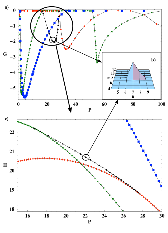
Figure 3: (Color online). Results for $\gamma=10$. (a) Smallest eigenvalue $G$ versus Power. (b) Profile of intermediate solution (IS). (c) Energy $H$ versus Power for the region enclosed with a circle in (a). Diamonds, stars, squares, and triangles represent OO, OE, EE, and IS solutions, respectively.

Compared to the previous case, for $\gamma=10$ (implying a higher nonlinearity or a lower coupling between sites) solutions are more localized as expected. The stability diagram is presented in Fig. 3(a). As in the former case, multiple exchange regions where two solutions are stable at the same level of power can be observed: OO-OE, OE-EE, EE-OO, EE-OE. It is very clear from Fig. 3(a) that the IS (Fig. 3(b)) exists in the exchange region where the OO and OE solutions are stable (region enclosed by a circle in Fig. 3(a)). In this case the differences in energies are bigger, and we show in Fig. 3(c) a plot for the Hamiltonian versus Power. In this figure the way in which the IS connect the OE and the OO solutions can be very well observed. Before the crossing point, the energy difference $\Delta H\equiv H_{\mathrm{OO}}-H_{\mathrm{OE}}$ is lower than zero. After the crossing point this difference has changed its sign. This is a clear confirmation that the oscillation in the PN potential, if defined in the “naive” way as $\Delta H$, is due to the exchange in the stability of different solutions. The OE solution becomes stable (see Fig. 3(a)), then it shares stability with the OO solution, and finally it continues to be stable while the OO solution becomes unstable. The same behavior is described by energy considerations from Fig. 3(c). Note however, that the actual energy barrier to overcome for a localized solution moving adiabatically in an axial direction is larger than $\Delta H$ in the regime of simultaneous OO and OE stability, if the path goes via the IS whose energy is larger. This will be illustrated in Sec. IV.

IV Mobility of two-dimensional localized solutions

We study the mobility of 2D discrete solitons by solving numerically Eq. (1) for initial conditions obtained by slightly perturbing the stationary solutions described above. To be specific, we here choose the OO solution and study mobility in regions where this profile is always stable. In our simulations, we always consider perturbations obtained by “kicking” the initial OO solutions using: $u_{n,m}(0)=u_{n,m}\exp[i\left(k_{x}n+k_{y}m\right)]$. Note that such perturbations do not change the power, but generally increase the energy compared to the stationary solutions.

In Fig. 4 we show dynamical results for $\gamma=4$ and $\gamma=10$. First, for $\gamma=4$, we study the dynamics for small-power solutions, $P\approx 4$. Fig. 4(a) shows the average axial position (4) for an OO profile (belonging to the branch with $\partial P/\partial\lambda>0$ in Fig. 1(d)) kicked in the axial direction. In this region of power the OO mode is stable, while the OE and EE modes are both unstable (see Fig. 2(a)). The additional energy due to the kick corresponds to $\Delta H=0.0038$, which is larger than the energy difference between the OO and OE configurations, $\Delta H=0.0032$. For this reason, the solution first begins to move, but is then trapped 4 sites away from the input center in a (stable) OO configuration. Due to radiation losses, it has not sufficient energy to overcome the next barrier, but instead begins to oscillate around its new center due to the excitation of its stable internal mode. An interesting detail in this result is the structure of the curve. When the OO mode propagates, it changes its form between the OO and OE profiles. It is clear from the figure that the maximum propagation velocity corresponds to the OO configuration (bigger slope, potential well), and the minimum velocity (slope $\approx 0$, saddle point) corresponds to the OE configuration (centered between two sites in the propagation direction). Similar results for 1D systems have been described, e.g., in Refs. Cretegny98 ; GJ03 .

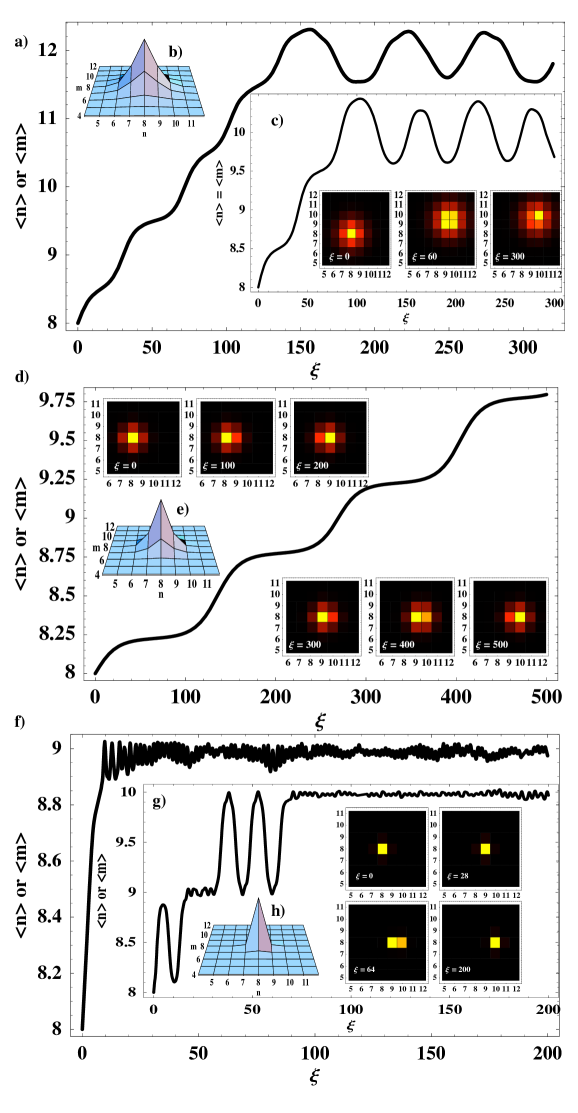
Figure 4: (Color online). Mobility results. $\gamma=4,\ P=3.99$: (a) axial propagation for $k_{x}$ or $k_{y}=0.0323$; (b) OO profile; (c) diagonal propagation for $k_{x}=k_{y}=0.031$. $\gamma=4,\ P=9.42$: (d) axial propagation for $k_{x}$ or $k_{y}=0.00624$; (e) OO profile. $\gamma=10$: (f) axial propagation for $k_{x}$ or $k_{y}=0.6$ ($P=20.43$); (g) axial propagation for $k_{x}$ or $k_{y}=0.5$ ($P=24.76$); (h) OO profile. System size $N=M=15$, periodic boundary conditions.

For the same parameter values, we illustrate in Fig. 4(c) the propagation of an OO profile kicked in the diagonal direction. This plot describes the identical evolution in both axes. It can be observed that the OO profile propagates in the diagonal direction, changing its form from an OO configuration to an EE one (see the inset). The final switching here was two sites in both directions, from the input position $\{8,8\}$ to $\{10,10\}$. Here, the maximum propagation velocities correspond to the OO configurations, and the almost zero velocities correspond to the EE configurations. As before, the soliton will not be able to continue its propagation because of the radiation losses. In this case, the diagonal kick corresponds to $\Delta H=0.007$, while the energy difference between OO and EE configurations at this power is $\Delta H=0.006$.

The dynamics shown in Figs. 4 (a) and (c) corresponds essentially to that of a typical 1D cubic DNLS case in the regime of low power, where the PN barrier is relatively small, and the site-centered solution possesses a symmetry-breaking internal translational mode (see, e.g., JAGCR98 ), which may be excited by kicking the solution. Now, if we compare with the 2D cubic DNLS case, the dynamics and the regions of existence of the stationary localized solutions are very different. First, in a P versus $\lambda$ diagram for the 2D cubic DNLS case 2Dkevre , there are different power thresholds for OO, OE, and EE solutions, far away separated in power. This implies that below a certain level of the power, it is not possible to move the OO profile since no OE or EE solution exists at the same power. If we consider a higher level of the power (on the high-frequency branch with a stable OO solution), where two or three solutions exist, the profiles are too localized and do not possess any localized symmetry-breaking internal modes. This implies also that the PN potential is large, and mobility is not possible by kicking the solutions since there are no internal translational ‘depinning’ modes to excite. Thus, for cubic 2D DNLS, mobility is possible only on the ‘continuumlike’ low-frequency branch with $\partial P/\partial\lambda<0$, where OO, OE, and EE solutions are all unstable, but such moving solutions will typically ‘quasicollapse’ into localized pinned solutions as described in Christiansen96 .

In the 2D saturable case, these thresholds still exist but are much closer in power. For $\gamma=4$, the power thresholds for different solutions are: $P_{\mathrm{OO}}\approx P_{\mathrm{OE}}\approx P_{\mathrm{EE}}\approx 3.07$ (cf. Fig. 1(d)). This means that all solutions have essentially the same power threshold value, and that we are in principle able to observe good mobility in the low-power regime of the branch with $\partial P/\partial\lambda>0$ for $P\gtrsim 3.08$. For $\gamma=10$, the differences in power are higher than in the previous case, but they are still rather small. The corresponding threshold values are (see Fig. 1(e)): $P_{\mathrm{OO}}=0.90$, $P_{\mathrm{OE}}=1.13$, and $P_{\mathrm{EE}}=1.17$. This behavior is another remarkable property of the saturable nonlinearity. As is wellknown (see, e.g., Flach ), in two-dimensional discrete nonlinear systems with an effectively cubic (or stronger) nonlinearity, a power threshold value always exists for localized solutions. Our results suggest that, increasing the value of $\gamma$, it is possible to decrease this power threshold value towards zero (for $\gamma=100$ this value is $P_{\mathrm{OO}}=0.059$). In the small-amplitude regime, the dynamics is essentially governed by the cubic term in the Taylor expansion of the saturable nonlinearity, and thus Eq. (1) is well approximated by the cubic DNLS model with effective nonlinearity parameter $\gamma P$. Thus, the threshold power should scale as $\gamma^{-1}$ for large $\gamma$. A similar result was also discussed in Ref. ZCR98 (see, e.g., Fig. 6 in this paper).

Now, we go further to study the exchange regions where we observe “multistability” of solutions. In the region of power shown in Fig. 2(b), we study the first exchange region between the OO and the OE solutions. In Fig. 4(d) we show the effect of kicking the OO solution in the axial direction. The energy added to the profile due to the kick is $\Delta H=0.0003$, and the energy difference between the OO and the OE configurations is $\Delta H=-0.0001$, i.e., the OE solution has the lowest energy. However, in this case there exists also an intermediate solution (Fig. 2(c)), which is important to explain the mobility we observe in this dynamics. The energy difference between the OO and the IS solutions is $\Delta H=0.0002$. In fact, the solution can move across the array as far as the radiation losses permits it. The regions in which the profile changes its velocity can clearly be observed in this figure. First, for the OO and the OE solutions the velocity has maxima, which is corresponding with the stability analysis where both solutions are stable. Both solutions correspond to a potential well in a dynamical representation. We can also note, that the velocity is larger at half-integer values than at integer values, consistent with the fact that the OE solution has lower energy than OO. The minimum velocities (slope $\approx 0$) clearly correspond to the IS between the OO and the OE profiles IS . For this case IS have shown to increase mobility, essentially because all solutions are very close in energy and just a little kick, corresponding to approximately the energy difference between the OO and IS, is required to move them. An analogous scenario would be seen by using the kicked stable OE solution as initial condition.

Finally, we study the case for $\gamma=10$. We first look for mobility in the same region of power as in the previous case ($P\approx 4$ and $P\approx 9$). For these powers we were not able to find mobility of localized solutions, essentially because the stationary solutions are distant in energy values.

Then, we study the first crossing point between the energy of the OO and the OE solutions (Fig. 3(c)). From the previous discussion, it is clear that in the exchange regions, the mobility of solutions depends on the IS. So, if we want to switch the profile in the lattice, we first have to overcome the energy barrier between the OO and the IS. We study two cases where we found some mobility. First, we take an OO profile for a power lower than the crossing point power ($P\approx 21.5$), i.e. $P_{\mathrm{OO}}=20.43$. For this power both solutions are stable, but the OO solution has lower energy than the OE solution. Therefore, we expect it to be most probable to have an OO stable configuration at the end of the process by switching the profile. However, if radiation losses are large, the solution might in principle also be trapped in a metastable OE configuration, since it might not have enough energy to overcome the barrier between OE and OO created by IS. In Fig. 4(f), we show an example of switching of an OO mode with one site along the axial direction. The energy due to the kick was $\Delta H=2.147$, the energy difference between the OO and the OE configurations was $\Delta H=0.370$, and the energy difference between the OO and the IS was $\Delta H=0.672$. The figure shows how the OO solution starts to move very fast (large slope), but it is not able to continue its movement in the array because of the high radiation losses of the switching process. This is a remarkable example of discrete switching in nonlinear lattices.

Now, we consider the situation where the OO power ($P_{\mathrm{OO}}=24.76$) is higher than the crossing point power. Here, both OO and OE solutions are stable, but the OE solution has lower energy, so from energetic arguments we would expect the most likely final profile to be an OE mode (however, depending on the amount of radiation losses, either an OE or an OO profile may be observed as final state as discussed above). The dynamics resulting from a kick of the OO mode producing a $\Delta H=2.045$ is illustrated in Fig. 4(g). The corresponding energy difference between the OO and the OE modes is $\Delta H=-1.120$, and between the OO mode and the IS, $\Delta H=0.118$. It is clear from these numbers that we need to supply the OO mode with some extra energy to move it across the array even though the energy for the OE solution is lower. This property is due to the oscillating behavior of the Hamiltonian. Without such crossing points, 2D mobility for high power solutions can generally not be expected because of the large PN barrier. Fig. 4(g) shows the switching of an OO solution with two sites in the axial direction from the input position. First, the OO solution has sufficient energy (big slope) to overcome the IS energy barrier. Then, its velocity increases as it passes the OE position, and then again it slows down when approaching the next IS (with central position close to site 9). Now, it does not have enough energy to overcome this barrier, and instead it makes one full oscillation around the OE position, limited by the two unstable IS. However, during this oscillation it has recovered some of its energy, and can now pass the IS barrier to the position of the next site, where it gets temporarily trapped into an OO configuration. The radiation losses are still not too high, and the OO mode being energetically unstable decays after a short distance $\xi$ into a state of large-amplitude oscillations around the energetically stable configuration, the OE mode centered in $\{9.5,8\}$ (see inset in Fig. 4(g)). Now the solution has enough energy to oscillate between two sites (9 and 10). This oscillation produces more radiation losses, and the final profile is an OO mode centered in the site number 10, trapped by the barrier created by its nearby IS. Figs. 4(b), (e), and (h) show different profiles in the different regions of mobility. It is clear from these figures that the mobility is enhanced for less localized solutions as expected from the PN potential concept, but it is not forbidden for highly localized solutions as we have shown.

We have checked these dynamical cases also for a bigger array, where $N=M=21$. The quantitative results shown in Fig. 4 change somewhat due to the extension of the system, but the qualitative picture for the soliton’s mobility is preserved. We set in our computations periodic boundary conditions, which implies that some radiation comes back perturbing the final state of the profile. Therefore, the results are dependent of the boundaries. However, the important issue we want to emphasize here is the mobility of highly 2D localized states, which is independent of the array size for saturable nonlinear media.

V Conclusions

In conclusion, we have analyzed in some detail the mechanisms leading to mobility of localized modes in a two-dimensional DNLS-type lattice with saturable nonlinearity. From a practical point of view, the most important result from our study is the drastic enhancement of the mobility resulting from the saturable nature of the nonlinearity, both for low-power and high-power excitations. This effect, which should be observable for two-dimensional waveguide arrays, is in our opinion more remarkable than the similar effect previously reported in 1D HMSK04 , since stable localized excitations for pure Kerr nonlinear media are known to be essentially immobile in 2D. Thus, the saturability of the nonlinearity introduces new possibilities for power controlled steering and switching also for 2D arrays. As we have shown, mobility is not restricted to axial directions, but also steering in diagonal directions is possible.

In principle, the choice of a smaller value of $\gamma$, for instance $\gamma=3$, could also be good for 2D mobility, because it is expected that the first stability exchange region occurs for lower level of power. However, it is important to notice that a decrease in the value of $\gamma$ (see Fig. 1) also implies an increasing value for the power threshold of the solutions, due to a balance between the nonlinearity and the coupling terms. We confirmed this behaviour for $\gamma=3$, where the power threshold was found to be $P\approx 4.84$, while the first stability exchange region was found to occur at $P\approx 6.98$. On the contrary, if we increase further the value of $\gamma$, for instance $\gamma=20$, we expect that the powers for the first exchange region will be much higher and, in this sense, it is not really interesting from the optical application point of view, which always requires low level of power.

From a more fundamental point of view, our results also give a deeper understanding for the mechanisms for mobility of localized modes. In particular, this concerns the relation between regimes of exchange of stability between site-centered and bond-centered stationary solutions, and points of vanishing of a so-called Peierls-Nabarro (PN) barrier defined naively as the difference between such solutions at constant norm. As we have shown, this definition is not appropriate in regimes where both these solutions are simultaneously stable, due to the existence of unstable intermediate solutions (IS) of higher energy. However, redefining the PN barrier as the energy difference to the relevant IS gave good agreement with the numerically observed additional energy necessary for making a stationary solution mobile. An analogous scenario should exist in 1D, and gives an intuitive explanation to why, in spite of the repeated vanishing of the “PN potential” reported in Ref. HMSK04 at several critical powers, the mobility is good only around the first of these Maluckov . At the other (larger) critical powers, the barriers created by the IS are expected to be very large, and no smooth path in phase space passing simultaneously close to all three stationary solutions is likely to exist.

It is also interesting to mention, that although, in 1D, both the existence of a particular class of IS (which were even obtained analytically) Khare04 , and the “PN barrier vanishing” HMSK04 were previously known for the saturable potentials, the connection between these results, and their relation to exchange of stability, seems so far to have gone unnoticed.

- (1) D.K. Campbell, S. Flach, and Yu.S. Kivshar, Phys. Today 57(1), 43 (2004).
- (2) A.A. Sukhorukov, Yu.S. Kivshar, H.S. Eisenberg, and Y. Silberberg, IEEE J. Quantum Electron. 39, 31 (2003).
- (3) D.N. Christodoulides, F. Lederer, and Y. Silberberg, Nature (London) 424, 817 (2003).
- (4) F. Chen, M. Stepić, C.E. Rüter, D. Runde, D. Kip, V. Shandarov, O. Manela, and M. Segev, Opt. Express 13, 4314 (2005).
- (5) M. Matuszewski, C.R. Rosberg, D.N. Neshev, A.A. Sukhorukov, A. Mitchell, M. Trippenbach, M.W. Austin, W. Krolikowski, and Yu. S. Kivshar, Opt. Express 14, 254 (2006).
- (6) H.S. Eisenberg, Y. Silberberg, R. Morandotti, A.R. Boyd, and J.S. Aitchison, Phys. Rev. Lett. 81, 3383 (1998); R. Morandotti, H.S. Eisenberg, Y. Silberberg, M. Sorel, and J.S. Aitchison, Phys. Rev. Lett. 86, 3296 (2001); D. Mandelik, R. Morandotti, J.S. Aitchison, and Y. Silberberg, Phys. Rev. Lett. 92, 093904 (2004).
- (7) J.W. Fleischer, T. Carmon, M. Segev, N.K. Efremidis, and D.N. Christodoulides, Phys. Rev. Lett. 90, 023902 (2003).
- (8) D. Neshev, E. Ostrovskaya, Y. Kivshar, and W. Krolikowski, Opt. Lett. 28, 710 (2003).
- (9) J.W. Fleischer, M. Segev, N.K. Efremidis, and D.N. Christodoulides, Nature 422, 147 (2003).
- (10) D.N. Christodoulides and R.I. Joseph, Opt. Lett. 13, 794 (1988).
- (11) J.C. Eilbeck and M. Johansson, in Localization and Energy Transfer in Nonlinear Systems, Proceedings of the Third Conference, San Lorenzo de El Escorial Madrid, edited by L. Vázquez, R.S. MacKay, and M.P. Zorzano (World Scientific, Singapore, 2003), p. 44; e-print nlin.PS/0211049.
- (12) N.K. Efremidis, S. Sears, D.N. Christodoulides, J.W. Fleischer, and M. Segev, Phys. Rev. E 66, 046602 (2002).
- (13) V.L. Vinetskii and N.V. Kukhtarev, Fiz. Tverd. Tela 16, 3714 (1974) [Sov. Phys. Solid State 16, 2414 (1975)].
- (14) M. Stepić, D. Kip, Lj. Hadz̆ievski, and A. Maluckov, Phys. Rev. E 69, 066618 (2004).
- (15) Lj. Hadz̆ievski, A. Maluckov, M. Stepić, and D. Kip, Phys. Rev. Lett. 93, 033901 (2004).
- (16) A. Khare, K.Ø. Rasmussen, M.R. Samuelsen, and A. Saxena, J. Phys. A: Math. Gen. 38, 807 (2005).
- (17) A. Maluckov, M. Stepić, D. Kip, and Lj. Hadz̆ievski, Eur. Phys. J. B 45, 539 (2005).
- (18) J. Cuevas and J.C. Eilbeck, e-print nlin.PS/0501050.
- (19) Yu. S. Kivshar and D.K. Campbell, Phys. Rev. E 48, R3077 (1993).
- (20) R. Morandotti, U. Peschel, J.S. Aitchison, H.S. Eisenberg, and Y. Silberberg, Phys. Rev. Lett. 83, 2726 (1999).
- (21) M. Öster, M. Johansson, and A. Eriksson, Phys. Rev. E 67, 056606 (2003).
- (22) T. Cretegny, Ph.D. thesis (in French), École Normale Supérieure de Lyon, 1998 (unpublished).
- (23) P.L. Christiansen, Yu.B. Gaididei, K.Ø. Rasmussen, V.K. Mezentsev, and J. J. Rasmussen, Phys. Rev. B 54, 900 (1996).
- (24) R.A. Vicencio, M.I. Molina, and Yu.S. Kivshar, Opt. Lett. 28, 1942 (2003); R.A. Vicencio, M.I. Molina, and Yu.S. Kivshar, Opt. Lett. 29, 2905 (2004).
- (25) R. Fischer, D. Träger, D.N. Neshev, A.A. Sukhorukov, W. Krolikowski, C. Denz, and Yu.S. Kivshar, e-print physics/0509255.
- (26) Y. Zolotaryuk, P.L. Christiansen, and J. J. Rasmussen, Phys. Rev. B 58, 14305 (1998).
- (27) A.S. Desyatnikov, D.N. Neshev, Yu.S. Kivshar, N. Sagemerten, D. Träger, J. Jägers, C. Denz, and Y.V. Kartashov, Opt. Lett. 30, 869 (2005).
- (28) J. Yang, New. J. Phys. 6, 47 (2004).
- (29) P.G. Kevrekidis, K.Ø. Rasmussen, and A.R. Bishop, Phys. Rev. E61, R2006 (2000).
- (30) V.K. Mezentsev, S.L. Musher, I.V. Ryzhenkova, and S.K. Turitsyn, JETP Lett. 60, 829 (1994); E.W. Laedke, K.H. Spatschek, V.K. Mezentsev, S.L. Musher, I.V. Ryzhenkova, and S.K. Turitsyn, JETP Lett. 62, 677 (1995).
- (31) S. Flach, K. Kladko, and R.S. MacKay, Phys. Rev. Lett. 78, 1207 (1997).
- (32) J. Carr and J.C. Eilbeck, Phys. Lett. A 109, 201 (1985).
- (33) A.V. Gorbach and M. Johansson, Phys. Rev. E 67, 066608 (2003).
- (34) M. Johansson, S. Aubry, Yu.B. Gaididei, P.L. Christiansen, and K.Ø. Rasmussen, Physica D 119, 115 (1998).
- (35) As a method to find numerically the exact IS, we take the dynamical profile for a certain (e.g., for Fig. 4(d)) of a kicked OO solution, and use it as a trial solution for the Newton-Raphson scheme to find stationary solutions for constructing the IS spectra in Figs. 2 and 3.
- (36) A. Maluckov (private communication).