Opinion formation and phase transitions in a probabilistic cellular automaton with two absorbing states

Abstract

We discuss the process of opinion formation in a completely homogeneous, democratic population using a class of probabilistic cellular automata models with two absorbing states. Each individual can have one of two opinions that can change according to that of his neighbors. It is dominated by an overwhelming majority and can disagree against a marginal one. We present the phase diagram in the mean field approximation and from numerical experiments for the simplest nontrivial case. For arbitrarily large neighborhoods we discuss the mean field results for a non-conformist society, where each individual adheres to the overwhelming majority of its neighbors and choses an opposite opinion in other cases. Mean field results and preliminary lattice simulations with long-range connections among individuals show the presence of coherent temporal oscillations of the population.

1 Modeling social pressure and political transitions

What happens to a society when a large fraction of people switches from a conformist to a non-conformist attitude? Is the transition smooth or revolutionary? These important questions, whose answers can make the difference between two well-known political points of view, is approached using a theoretical model, in the spirit of Latané’s social impact theory [1, 2].

We assume that one’s own inclination towards political choices originates from a mixture of a certain degree of conformism and non-conformism. Conformists tend to agree with the local community majority, that is with the average opinion in a given neighborhood, while non-conformists do the opposite. However, an overwhelming majority in the neighborhood (which includes the subject itself) is always followed.

We shall study here the case of a homogeneous population, i.e. a homogeneous democratic society. It may be considered as the annealed version of a real population, which is supposedly composed by a mixture of conformist and non-conformist people who do not change easily their attitude.

In Sec. 2 we introduce a class of probabilistic cellular automata characterized by the size $2r+1$ of the neighborhood, a majority threshold $q$, a coupling constant $J$ and an external field $H$.

We are interested in the two extreme cases: people living on a one-dimensional lattice, interacting only with their nearest neighbors ($r=1$) and people interacting with a mean-field opinion.

In Sec. 3 we present the simplest case where each individual interacts with his two nearest neighbors ($r=1$), the mean field phase diagram and the one found from numerical experiments. For this simple case, we find a complex behavior which includes first and second order phase transitions, a chaotic region and the presence of two universality classes [6]. In Sec. 4 we discuss the mean field behavior of the model for arbitrary neighborhoods and majority thresholds when the external field is zero and the coupling constant is negative (non-conformist society). The phase diagram of the model exhibits a large region of coherent temporal oscillations of the whole populations, either chaotic or regular. These oscillations are still present in the lattice version with a sufficient large fraction of long-range connections among individuals, due to the small-world effect [7].

2 The model

We denote by $x_{i}^{t}$ the opinion assumed by individual $i$ at time $t$. We shall limit to two opinions, denoted by $-1$ and $1$ as usual in spin models. The system is composed by $L$ individuals arranged on a one-dimensional lattice. All operations on spatial indices are assumed to be modulo $L$ (periodic boundary conditions). The time is considered discontinuous (corresponding, for instance, to election events). The state of the whole system at time $t$ is given by $\boldsymbol{x}^{t}=(x_{0}^{t},\dots,x_{L-1}^{t})$ with $x_{i}^{t}\in\{-1,1\}$;

The individual opinion is formed according to a local community “pressure” and a global influence. In order to avoid a tie, we assume that the local community is formed by $2r+1$ individuals, counting on equal ground the opinion of the individual himself at previous time. The average opinion of the local community around site $i$ at time $t$ is denoted by $m^{t}_{i}=\sum_{j=-r}^{r}x^{t}_{i+j}$.

The control parameters are the probabilities $p_{s}$ of choosing opinion $1$ at time $t+1$ if this opinion is shared by $s$ people in the local community, i.e.  if the local “field” is $m=2s-2r-1$.

Let $J$ be a parameter controlling the influence of the local field in the opinion formation process and $H$ be the external social pressure. The probability $p_{s}$ are given by

$$p_{s}=p_{(m+2r+1)/2}\propto\exp(H+Jm).$$

One could think to $H$ as the television influence, and $J$ as educational effects. $H$ pushes towards one opinion or the other, and people educated towards conformism will have $J>0$, while non-conformists will have $J<0$. In the statistical mechanics lingo, all parameters are rescaled to include the temperature.

The hypothesis of alignment to overwhelming local majority is represented by a parameter $q$, indicating the critical size of local majority. If $s<q$ ($m<2q-2r-1$), then $x_{i}^{t+1}=-1$, and if $s>2r+1-q$ ($m>2r+1-2q$), then $x_{i}^{t+1}=1$.

In summary, the local transition probabilities of the model are

$$p_{s}=\begin{cases}0&\text{if $s<q$;}\\ \dfrac{\mathcal{A}\mathcal{B}^{s}}{1+\mathcal{A}\mathcal{B}^{s}}&\text{if $q\leq s\leq 2r+1-q$;}\\ 1&\text{if $s>2r+1-q$;}\end{cases}$$ (1)

where $\mathcal{A}=\exp[2H+2J(2r-1)]$ and $\mathcal{B}=\exp(4J)$.

For $q=0$ the model reduces to an Ising spin system. For all $q>0$ we have two absorbing homogeneous states, $\boldsymbol{x}=\boldsymbol{-1}$ ($c=0$) and $\boldsymbol{x}=\boldsymbol{1}$ ($c=1$) corresponding to infinite coupling (or zero temperature) in the statistical mechanical sense. With these assumptions, the model reduces to a one-dimensional, one-component, totalistic cellular automaton with two absorbing states.

The order parameter is the fraction $c$ of people sharing opinion $1$.  It is zero or one in the two absorbing states, and assumes other values in the active phase. The model is symmetric since the two absorbing states have the same importance.

3 A simple case

Let us study the model for the simplest, nontrivial case: one dimensional lattice, $r=1$ and $q=1$. We have a probabilistic cellular automaton with three inputs, and two free control parameters, $p_{1}$ and $p_{2}$, while $p_{0}\equiv 0$ and $p_{3}\equiv 1$, according to Eq. (1).

One can also invert the relation between $(H,J)$ and $(p_{1},p_{2})$:

$$H=\dfrac{1}{4}\log\left(\dfrac{p_{1}p_{2}}{(1-p_{1})(1-p_{2})}\right),\qquad J=\dfrac{1}{4}\log\left(\dfrac{p_{2}(1-p_{1})}{p_{1}(1-p_{2})}\right).$$

The diagonal $p_{2}=p_{1}$ corresponds to $J=0$ and the diagonal $p_{2}=1-p_{1}$ to $H=0$.

At the boundaries of probability intervals, we have four deterministic (elementary) cellular automata, that we denote T3, T23, T13 and T123, where the digits indicate the values of $s$ for which $p_{s}=1$ [8].

Rule T3 (T123) brings the system into the $c=0$ ($c=1$) absorbing state except for the special case of the initial configuration homogeneously composed by the opposite opinion.

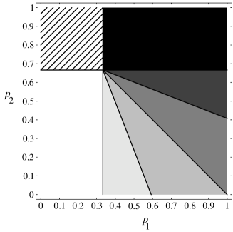
Figure 1: Mean-field phase diagram for the density $c$ coded as gray levels ranging from white ($c=0$) to black ($c=1$). The dashed upper-left region denotes the coexistence phase, in which both states $c=0$ and $c=1$ are stable, and the final state depends on the initial density (first-order transition).

Rule T23 is a strict majority rule, whose evolution starting from a random configuration leads to the formation of frozen patches of zeros and ones in a few time steps. A small variation of the probabilities induces fluctuations in the position of the patches. Since the patches disappear when the boundaries collide, the system is equivalent to a model of annihilating random walks, which, in one dimensions, evolves towards one of the two absorbing states according to the asymmetries in the probabilities or in the initial configuration.

Rule T13 on the other hand is a “chaotic” one,  leading to irregular pattern for almost all initial conditions (except for the absorbing states). These patterns are microscopically very sensitive to perturbations, but very robust for what concerns global quantities (magnetization).

The role of frustrations (the difficulty of choosing a stable opinion) is evidentiated by the following considerations. Rule T23 corresponds to a ferromagnetic Ising model at zero temperature, so an individual can simply align with the local majority with no frustrations. On the contrary, rule T13 is unable to converge towards an absorbing state (always present), because these states are unstable: a single individual disagreeing with the global opinion triggers a flip in all local community to which he/she belongs to. It is possible to quantify these concepts by defining stability parameters similar to Lyapunov exponents [10].

We start by studying the mean-field approximation for the generic case, with $p_{1}$ and $p_{2}$ different from zero or one.

Let $c$ and $c^{\prime}$ denote the density of opinion $1$ at times $t$ and $t+1$ respectively. We have

$$c^{\prime}=3p_{1}c\left(1-c\right)^{2}+3p_{2}c^{2}\left(1-c\right)+c^{3}.$$

This map has three fixed points, the state $\boldsymbol{x}=\boldsymbol{-1}$ ($c=0$), the state $\boldsymbol{x}=\boldsymbol{1}$ ($c=1$) and a microscopically disordered state ($0\leq c\leq 1$). The model is obviously symmetric under the changes $p_{1}\to 1-p_{2}$, $p_{2}\to 1-p_{1}$ and $x\to 1-x$, implying a fundamental equivalence of political opinions in this model. The stability of fixed points marks the different phases, as shown in Fig. 1.

The stability of the state $c=1$ ($c=0$) corresponds to large social pressure towards opinion $1$ ($-1$). The value of $J$ determines if a change in social pressure corresponds to a smooth or abrupt transition.

3.1 Phase transitions and damage spreading in the lattice case

The numerical phase diagram of the model starting from a random initial state with $c^{0}=0.5$ is shown in Fig. 2. The scenario is qualitatively the same as predicted by the mean-field analysis. In the upper-left part of the diagram both states $c=0$ and $c=1$ are stable. In this region the final fate of the system depends on the initial configuration.

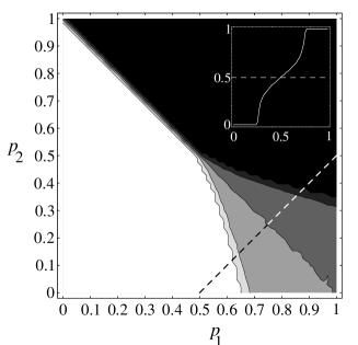
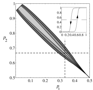
Figure 2: Numerical phase diagram for the density $c$ (left) and hysteresis region for several values of the noise $\epsilon$ and relaxation time $T$ (right). Same color code as in Figure 1.

Due to the symmetry of the model, the two second-order phase transition curves meet at a bicritical point $(p_{t},1-p_{t})$ where the first-order phase transition line ends. Crossing the second-order phase boundaries on a line parallel to the diagonal $p_{1}=p_{2}$, the density $c$ exhibits two critical transitions, as shown in the inset of the right panel of Fig. 2. Approaching the bicritical point the critical region becomes smaller, and corrections to scaling increase. Finally, at the bicritical point, the two transitions coalesce into a single discontinuous (first-order) one.

First-order phase transitions are usually associated to a hysteresis cycle due to the coexistence of two stable states. To visualize the hysteresis loop (inset of the right panel of Fig. 2) we modify the model slightly by letting $p_{0}=1-p_{3}=\epsilon$ with $\epsilon\ll 1$. In this way the configurations $\boldsymbol{x}=\boldsymbol{-1}$ and $\boldsymbol{x}=\boldsymbol{1}$ are no longer absorbing. This brings the model back into the class of equilibrium models for which there is no phase transition in one dimension but metastable states can nevertheless persist for long times. The width of the hysteresis cycle, shown in the right panel of Fig. 2, depends on the value of $\epsilon$ and the relaxation time $T$.

We study the asymptotic density as $p_{1}$ and $p_{2}$ move on a line with slope 1 inside the dashed region of Fig. 1. For $p_{1}$ close to zero, the model has only one stable state, close to the state $c=0$. As $p_{1}$ increases adiabatically, the new asymptotic density will still assume this value even when the state $c=1$ become stable. Eventually the first state become unstable, and the asymptotic density jumps to the stable fixed point close to the state $c=1$. Going backwards on the same line, the asymptotic density will be close to one until that fixed point disappears and it will jump back to a small value close to zero.

Although not very interesting from the point of view of opinion formation models, the problem of universality classes in the presence of absorbing states have attracted a lot of attention by the theoretical physics community in recent years [11, 12]. For completeness we report here the main results [6].

It is possible to show that on the symmetry line one can reformulate the problem in terms of the dynamics of kinks between patches of empty and occupied sites. Since the kinks are created and annihilated in pairs, the dynamics conserves the initial number of kinks modulo two. In this way we can present an exact mapping between a model with symmetric absorbing states and one with parity conservation.

Outside the symmetry line the system belongs to the directed percolation universality class [13]. We performed simulations starting either from one and two kinks. In both cases $p_{t}=0.460(2)$, but the exponents were found to be different. Due to the conservation of the number of kinks modulo two, starting from a single site one cannot observe the relaxation to the absorbing state, and thus $\delta=0$. In this case $\eta=0.292(5)$, $z=1.153(5)$. On the other hand, starting with two neighboring kinks, we find $\eta=0.00(2)$, $\delta=0.285(5)$, and $z=1.18(2)$. These results are consistent with the parity conservation universality class [3,4].

Let us now turn to the sensitivity of the model to a variation in the initial configuration, i.e. to the study of damage spreading or, equivalently, to the location of the chaotic phase. Given two replicas ${\boldsymbol{x}}$ and ${\boldsymbol{y}}$, we define the difference ${\boldsymbol{w}}$ as ${\boldsymbol{w}}={\boldsymbol{x}}\oplus{\boldsymbol{y}}$, where the symbol $\oplus$ denotes the sum modulus two.

The damage $h$ is defined as the fraction of sites in which $w=1$, i.e. as the Hamming distance between the configurations ${\boldsymbol{x}}$ and ${\boldsymbol{y}}$. We study the case of maximal correlations by using just one random number per site, corresponding to the smallest possible chaotic region [14].

In Fig. 3 the region in which the damage spreads is shown near the lower-right corner (chaotic domain). Outside this region small spots appear near the phase boundaries, due to the divergence of the relaxation time (second-order transitions) or because a small difference in the initial configuration can bring the system to a different absorbing state (first-order transition). The chaotic domain is stable regardless of the initial density. On the line $p_{2}=0$ the critical point of the density and that of the damage spreading coincide.

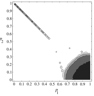
Figure 3: Phase diagram for the damage found numerically by considering the evolution starting from uncorrelated configurations with initial density equal to 0.5.

3.2 Reconstruction of the potential

An important point in the study of systems exhibiting absorbing states is the formulation of a coarse-grained description using a Langevin equation. It is generally accepted that the directed percolation universal behavior is represented by

$$\dfrac{\partial c(x,t)}{\partial t}=ac(x,t)-bc^{2}(x,t)+\nabla^{2}c(x,t)+\sqrt{c(x,t)}\alpha(x,t),$$

where $c(x,t)$ is the density field, $a$ and $b$ are control parameters and $\alpha$ is a Gaussian noise with correlations $\langle\alpha(x,t)\alpha(x^{\prime},t^{\prime})\rangle=\delta_{x,x^{\prime}}\delta_{t,t^{\prime}}$. The diffusion coefficient has been absorbed into the parameters $a$ and $b$ and the time scale.

It is possible to introduce a zero-dimensional approximation to the model by averaging over the time and the space, assuming that the system has entered a metastable state. In this approximation, the size of the original systems enters through the renormalized coefficients $\overline{a}$, $\overline{b}$,

$$\dfrac{\partial c(x,t)}{\partial t}=\overline{a}c(x,t)-\overline{b}c^{2}(x,t)+\sqrt{c(x,t)}\alpha(x,t),$$

where also the time scale has been renormalized.

The associated Fokker-Planck equation is

$$\dfrac{\partial P(c,t)}{\partial t}=-\dfrac{\partial}{\partial c}(\overline{a}c-\overline{b}c^{2})P(c,t)+\dfrac{1}{2}\dfrac{\partial^{2}}{\partial c^{2}}cP(c,t),$$

where $P(c,t)$ is the probability of observing a density $c$ at time $t$. One possible solution is a $\delta$-peak centered at the origin, corresponding to the absorbing state.

By considering only those trajectories that do not enter the absorbing state during the observation time, one can impose a detailed balance condition, whose effective agreement with the actual probability distribution has to be checked a posteriori. The effective potential $V$ is defined as $V(c)=-\log(P(c))$ and can be found from the actual simulations.

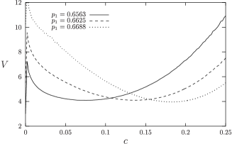
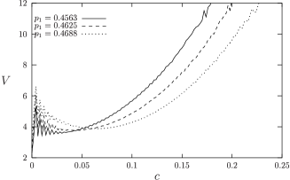
Figure 4: Reconstruction of potential $V(c)$ for $p_{2}=0$ (left) and for the kink dynamics on the line $p_{2}=1-p_{1}$ (right).

Figure 5: Case $H=0$, $J=-\infty$: the mean field map Eq. (2) (left) for $r=10$ and $q=2$ and the mean-field $r-q$ phase diagram (right). In the phase diagram the absorbing states are always present. Points mark parameter values for which the absorbing states are the only stable attractors. A plus sign denotes period-2 temporal oscillations between absorbing states, a star denotes the presence of a stable point at $c=0.5$, a cross (circle) denotes period-two (four) oscillations between two non-zero and non-one densities, triangles denote chaotic oscillations.

In the left panel of Fig. 4 we show the profile of the reconstructed potential $V$ for some values of $p$ around the critical value on the line $p_{2}=0$, over which the model belongs to the DP universality class. One can observe that the curve becomes broader in the vicinity of the critical point, in correspondence of the divergence of critical fluctuations $\chi\sim|p-p_{c}|^{-\gamma^{\prime}}$, $\gamma^{\prime}=0.54$ [15]. By repeating the same type of simulations for the kink dynamics (random initial condition), we obtain slightly different curves, as shown in the right panel of Fig. 4. We notice that all curves have roughly the same width. Indeed, the exponent $\gamma^{\prime}$ for systems in the PC universality class is believed to be exactly $0$ [16], as given by the scaling relation $\gamma^{\prime}=d\nu_{\perp}-2\beta$ [15]. Clearly, much more information can be obtained from the knowledge of $P(c)$, either by direct numerical simulations or dynamical mean field trough finite scale analysis, as shown for instance in Ref. [17].

4 Larger neighborhoods

In order to study the effects of a larger neighborhood and different threshold values $q$, let us start with the well known two-dimensional “Vote” model. It is defined on a square lattice, with a Moore neighborhood composed by 9 neighbors, synthetically denoted M in the following [8]. If a strict majority rule $q=4$ is applied (rule M56789, same convention as in Sec. 2) to a random initial configuration, one observes the rapid quenching of small clusters of ones and zero, similar to what happens with rule T23 in the one-dimensional case. A small noise quickly leads the system to an absorbing state. On the other hand, a small frustration $q=3$ (rule M46789) for an initial density $c^{0}=0.5$ leads to a metastable point formed by patches that evolve very slowly towards one of the two absorbing states. However, this metastable state is given by the perfect balance among the absorbing states. If one starts with a different initial “magnetization”, one of the two absorbing phases quickly dominates, except for small imperfections that disappear when a small noise is added.

In the general case, the mean-field equation is

$$c^{\prime}=\sum_{s=0}^{2r+1}\binom{2r+1}{s}c^{s}(1-c)^{2r+1-s}p_{s},$$ (2)

sketched in the left panel of Fig. 5.

We studied the asymptotic behavior of this map for different values of $r$ and $q$. For a given $r$ there is always a critical $q_{c}$ value of $q$ for which the active phase disappears, with an approximate correspondence $q_{c}\simeq 4/5r$. The active phase is favored by the presence of frustrations and the absence of the external pressure, i.e. for $J<0$ and $H=0$. We performed extensive computations for the extreme case $J=-\infty$, $H=0$ corresponding to a society of non-conformists without television. As shown in the right panel of Fig. 5, by increasing the neighborhood size $r$, one starts observing oscillations in the equilibrium process. This is evident in the limit of infinite neighborhood: the parallel dynamics induced by elections (in our model) makes individual tend to disalign from the marginal majority, originating temporal oscillations that can have a chaotic character. Since the absorbing states are present, and they are stable for $q>0$, the coherent oscillations of the population can bring the system into one absorbing state. This is reflected by the “hole” in the active phase in the mean field phase diagram.

Preliminary lattice simulations (not shown) reveal that this behavior is still present if there is a sufficiently large fraction of long-range connections due to the small-world effect [7], while the active phase is compact in the short-range case.

5 Conclusions

Although this model is quite rough, there are aspects that present some analogies with the behavior of a real society. In particular, the role of education, represented by the $J$ parameter. In a society dominated by conformists, the transitions are difficult and catastrophic, while in the opposite case of non-conformist people the transitions are smooth. However, in the latter case a great social pressure is needed to gain the majority.

On the other hand, if the neighborhood is large and non-conformism is present, one can observe the phenomenon of political instabilities given by temporal oscillations of population opinion, which could be interpreted as a symptom of healthy democracy.

References

- [1] Latané, B.: American Psychologist 36 (1981) 343
- [2] Galam, S., Gefen, Y., Shapir, Y.: Math. J. of Sociology 9, (1982) 1
- [3] Holyst, J.A., Kacperski, K, Schweitzer, F.: Physica A 285 (2000) 199
- [4] Galam, S., Chopard, B., Masselot, A., Droz, M.: Eur. Phys. J. B 4, (1998) 529
- [5] Chopard, B., Droz, M., Galam, S.: Eur. Phys. J. B 16, (2000) 575
- [6] Bagnoli, F., Boccara, N., Rechtman, R.: Phys. Rev. E 63 (2001) 46116 ; cond-mat/0002361
- [7] Watts, D. J., Strogatz S. H.: Nature 393 (1998) 440
- [8] Vichniac, G. Y.: Cellular Automata Models of Disorder and Organization In Bienestok, E., Fogelman, F., Weisbuch, G. (eds.), Disordered Systems and Biological Organization, NATO ASI Series, b F20/b, Berlin: Springer Verlag (1986) pp. 283-293; http://www.fourmilab.ch/cellab/manual/cellab.html
- [9] Wolfram, S.: Rev. Mod. Phys. 55 (1983) 601
- [10] Bagnoli, F., Rechtman, R., Ruffo, S.: Phys. Lett. A 172 (1992) 34 (1992).
- [11] Grassberger, P., von der Twer, T.: J. Phys. A: Math. Gen. 17 (1984) L105; Grassberger, P.: J. Phys. A: Math. Gen. 22 (1989) L1103
- [12] Hinrichsen, H. Phys. Rev. E 55 (1997) 219
- [13] Kinzel, W. In Deutsch, G., Zallen, R., Adler, J. (eds.): Percolation Structures and Processes, Adam Hilger, Bristol (1983); Kinzel, E., Domany, W.: Phys. Rev. Lett. 53 (1984) 311 ; Grassberger, P.: J. Stat. Phys. 79 (1985) 13
- [14] Hinrichsen, H., Weitz, J.S., Domany, E.: J. Stat. Phys. 88 (1997) 617
- [15] Muñoz, M.A., Dickman, R., Vespignani, A., Zapperi, S.: Phys. Rev. E 59 (1999) 6175
- [16] Jensen, I.: Phys. Rev. E 50 (1994) 3263
- [17] Jensen, I., Dickman, R., Phys. Rev. E 48 (1993) 1710