Introduction to Statistical Theory of Fluid Turbulence

Abstract

This is a brief introduction to the statistical theory of hydrodynamic turbulence with an emphasis on its field-theoretic treatment.

I Introduction

Fluid and plasma flows exhibit complex random behaviour at high Reynolds number; this phenomena is called turbulence. On the Earth, turbulence is observed in atmosphere, channel and rivers flows etc. In the universe, most of the astrophysical systems are turbulent. Some of the examples are solar wind, convective zone in stars, galactic plasma, accretion disk etc.

Reynolds number, defined as $UL/\nu$ ($U$ is the large-scale velocity, $L$ is the large length scale, and $\nu$ is the kinematic viscosity), has to be large (typically 2000 or more) for turbulence to set in. At large Reynolds number, there are many active modes which are nonlinearly coupled. These modes show random behaviour along with rich structures and long-range correlations. Presence of large number of modes and long-range correlations makes turbulence a very difficult problem that remains largely unsolved for more than hundred years.

Fortunately, random motion and presence of large number of modes make turbulence amenable to statistical analysis. Note that the energy supplied at large-scales $(L)$ gets dissipated at small scales, say $l_{d}$. Experiments and numerical simulations show that the velocity difference $u(\mathbf{x+l})-u(\mathbf{x})$ has a universal probability density function (pdf) for $l_{d}\ll l\ll L$. That is, the pdf is independent of experimental conditions, forcing and dissipative mechanisms etc. Kolmogorov (1941a, b, c). Because of its universal behaviour, the above quantity has been of major interest among physicists for many years. Unfortunately, we do not yet know how to derive the form of this pdf from the first principle, but some of the moments have been computed analytically. The range of scales $l$ satisfying $l_{d}\ll l\ll L$ is called inertial range.

In 1941 Kolmogorov Kolmogorov (1941a, b, c) computed an exact expression for the third moment of velocity difference. He showed that under vanishing viscosity, third moment for velocity difference for homogeneous, isotropic, incompressible, and steady-state fluid turbulence is

$$\left\langle\left(u_{||}(\mathbf{x+l})-u_{||}(\mathbf{x})\right)^{3}\right\rangle=\frac{4}{5}\Pi l$$

where $||$ is the parallel component along $\mathbf{l}$, $\left\langle.\right\rangle$ stands for ensemble average, and $\Pi$ is the energy cascade rate, which is also equal to the energy supply rate at large scale $L$ and the dissipation rate at the small scale $l_{d}$. Assuming fractal structure for the velocity field, and $\Pi$ to be constant for all $l$, it has been shown that the energy spectrum $E(k)$ is

$$E(k)=K_{Ko}\Pi^{2/3}k^{-5/3},$$

where $K_{Ko}$ is a universal constant, called Kolmogorov’s constant, and $L^{-1}\ll k\ll l_{d}^{-1}$. Numerical simulations and experiments verify the above energy spectrum apart from a small deviation called intermittency correction.

Availability of powerful computers and sophisticated theoretical tools have helped us understand several aspects of fluid turbulence. Some of these theories have been motivated by Kolmogorov’s theory for fluid turbulence. Note that incompressible turbulence is better understood than compressible turbulence. Therefore, our discussion is primarily for incompressible plasma. In this paper we focus on the universal statistical properties of fluid turbulence, which are valid in the inertial range. In this paper we will review the statistical properties of following quantities:

1. Inertial-range energy spectrum for fluid turbulence.

2. Various energy fluxes in fluid turbulence.

3. Energy transfers between various wavenumber shells.

4. Fluctuations in the energy flux

Many analytic calculations in fluid have been done using field-theoretic techniques. Even though these methods are plagued with some inconsistencies, many meaningful results have been obtained using them. Here we will discuss items 1-3 in some detail.

As mentioned above, pdf of velocity difference in fluid turbulence is still unsolved. We know from experiments and simulation that pdf is close to Gaussian for small $\delta u$, but is nongaussian for large $\delta u$. This phenomena is called intermittency. Note that various moments called Structure functions are connected to pdf. It can be shown that the structure functions are related to the “local energy cascade rate” $\Pi(k)$. Some phenomenological models, notably by She and Leveque She et al. (1993) based on log-Poisson process, have been developed to compute $\Pi(k)$; these models quite successfully capture intermittency in both fluid and MHD turbulence. The predictions of these models are in good agreement with numerical results.

Numerical simulations have provided many important data and clues for understanding the dynamics of turbulence. They have motivated new models, and have verified/rejected existing models. In that sense, they have become another type of experiment, hence commonly termed as numerical experiments. Modern computers have made reasonably high resolution simulations possible Gotoh (2002); Yeung et al. (2015); Ishihara et al. (2016); Verma et al. (2018)). Note that simulations are also used heavily for studying fluid flows around aircrafts and vehicles, in atmospheres, engineering devices like turbines etc.

Fluid turbulence has a larger volume of literature. Here we will list only some of them: Kraichnan (1959), Monin and Yaglom Monin and Yaglom (2007a, b), Leslie Leslie (1973), McComb McComb (1990, 2004, 2014); McComb and Watt (1992), Zhou et al. (1997), Zhou (2010), Yakhot and Orszag (1986), and Smith and Woodruff (1998) have reviewed field-theoretic treatment of fluid turbulence. The books by Frisch (1995), Lesieur (2008), Davidson (2004), and Verma (2019) cover recent developments and phenomenological theories. Also, the review articles by Orszag Orszag (1973), Kraichnan and Montgomery Kraichnan and Montgomery (1980), Sreenivasan Sreenivasan (1999), Verma (2004), and Alexakis and Biferale (2018) are quite exhaustive.

The outline of the paper is as follows: Section II contains definition of various global and spectral quantities along with their governing equations. In Section III we discuss the formalism of “mode-to-mode” energy transfer rates in fluid turbulence. Using this formalism, formulas for energy fluxes and shell-to-shell energy transfer rates have been derived. Section IV contains the existing discussion on Kolmogorov’s phenomenology for fluid turbulence. Sections V and VI contains very brief introduction on experiments and simulations in fluid turbulence. In Section VII we introduce Renormalization-group analysis of turbulence, with an emphasis on McComb’s procedure. In Section VIII we compute various energy fluxes and shell-to-shell energy transfers in fluid turbulence using field-theoretic techniques. Section IX contains a brief description of K41 theory, while Sec. X contains a intermittency models of fluid turbulence. Section XI describes the properties of the structure functions for 2D turbulence. Appendix A contains the definitions of Fourier series and transforms of fields in homogeneous turbulence. Appendix B contains the Feynman diagrams for fluid turbulence; these diagrams are used in the field-theoretic calculations. In the last two Appendix (C and D) we briefly mention the mode-to-mode energy transfer formalism for scalar and Rayleigh-Bénard convection.

II Governing equations

II.1 Equations for Fluid Dynamics

Navier-Stokes Equation

$$\frac{\partial\mathbf{u}}{\partial t}+(\mathbf{u}\cdot\nabla)\mathbf{u}=-\frac{1}{\rho}\nabla p_{th}+\nu\nabla^{2}\mathbf{u}+\frac{2\nu}{3}\nabla\nabla\cdot\mathbf{u},$$ (1)

where $p_{th}$ is called thermodynamic pressure. The law of mass conservation yields the following equation for density field $\rho(\mathbf{x})$

$$\frac{\partial\rho}{\partial t}+\nabla\cdot\left(\rho\mathbf{u}\right)=0$$ (2)

Pressure can be computed from $\rho$ using the equation of state

$$p=f\left(\rho\right)$$ (3)

This completes the basic equations of fluids. Using these equations we can determine the unknowns $(\mathbf{u,}\rho,p)$. Note that the number of equations and unknowns are the same.

On nondimensionalization of the Navier-Stokes equation, the term $\nabla p$ becomes $\left(d\rho/dx^{\prime}\right)/\rho$ $\times$ $(C_{s}/U)^{2}$, where $C_{s}$ is the sound speed, $U$ is the typical velocity of the flow, $x^{\prime}$ is the position coordinate normalized with relative to the length scale of the system Tritton (1988). $C_{s}\rightarrow\infty$ is the incompressible limit, which is widely studied because water, the most commonly found fluid on earth, is almost incompressible ($\delta\rho/\rho<$0.01) in most practical situations. The other limit $C_{s}\rightarrow 0$ or $U\gg C_{s}$ (supersonic) is the fully compressible limit, and it is described by Burgers equation that exhibits $k^{-2}$ energy spectrum. The energy spectrum for both these extreme limits well known. When $U/C_{s}\ll 1$ but nonzero, then we call the fluid to be nearly incompressible; Zank and Matthaeus Zank and Matthaeus (1990, 1991) have given theories for this limit. The energy and density spectra are not well understood for arbitrary $U/C_{s}$.

For most part of this paper, we assume the fluid to be incompressible. In most of the terrestrial experiments, the speed of water or air is less than the sound speed. Hence, incompressibility is a good assumption that simplifies the calculations significantly. The incompressibility approximation can also be interpreted as the limit when volume of a fluid parcel will not change along its path, that is, $d\rho/dt=0$. From the continuity equation (2), the incompressibility condition reduces to

$$\nabla\cdot\mathbf{u}=0$$ (4)

This is a constraint on the velocity field u. Note that incompressibility does not imply constant density. However, for simplicity we take density to be constant and equal to 1. Under this condition, Eqs. (1, 2) reduce to

$$\frac{\partial\mathbf{u}}{\partial t}+(\mathbf{u}\cdot\nabla)\mathbf{u} = -\nabla p+\nu\nabla^{2}\mathbf{u},$$ (5)

$$\nabla\cdot\mathbf{u} = 0.$$ (6)

When we take divergence of the equation Eq. (5), we obtain Poisson’s equation

$$-\nabla^{2}p=\nabla\cdot\left[(\mathbf{u}\cdot\nabla)\mathbf{u}\right].$$ (7)

Hence, given u fields at any given time, we can evaluate $p$. Hence $p$ is a dependent variable in the incompressible limit.

The Navier-Stokes equation is nonlinear, and that is the crux of the problem. The viscous $(\nu\nabla^{2}\mathbf{u)}$ term dissipates the input energy. The ratio of the nonlinear vs. viscous dissipative term is called Reynolds number $Re=UL/\nu$, where $U$ is the velocity scale, and $L$ is the length scale. For turbulent flows, Reynolds number should be high, typically more than 2000 or so Lesieur (2008).

II.2 Energy Equations and Conserved Quantities

In this subsection we derive energy equations for compressible and incompressible fluids. For compressible fluids we can construct equations for energy using Eq. (1). Following Landau Landau and Lifshitz (1987) we derive the following energy equation for the kinetic energy

$$\frac{\partial}{\partial t}\left(\frac{1}{2}\rho u^{2}+\rho\epsilon\right)=-\nabla\cdot\left[\left(\frac{1}{2}u^{2}+\epsilon\right)\rho\mathbf{u}\right]-\nabla\cdot(p\mathbf{u})+\Phi$$ (8)

where $\epsilon$ is the internal energy function. The first term in the RHS is the energy flux, and the second term is the work done by the pressure, which enhances the energy of the system. The third term,$\Phi$, a complex function of strain tensor, is the energy change due to surface forces.

In the above equations we apply isoentropic and incompressibility conditions. For the incompressible fluids we can choose $\rho=1$. Landau Landau and Lifshitz (1987) showed that under this condition $\epsilon$ is a constant. Hence, for incompressible fluid we treat $(u^{2})/2$ as total energy. For ideal incompressible fluid ($\nu=0)$ the energy evolution equation is

$$\frac{\partial}{\partial t}\frac{1}{2}\left(u^{2}\right)=-\nabla\cdot\left[\left(\frac{1}{2}u^{2}+p\right)\mathbf{u}\right]$$ (9)

By applying Gauss law we find that

$$\frac{\partial}{\partial t}\int\frac{1}{2}\left(u^{2}\right)d\mathbf{x}=-\oint\left[\left(\frac{1}{2}u^{2}+p\right)\mathbf{u}\right]\cdot d\mathbf{S}$$ (10)

For the boundary condition $u_{n}=0$ or periodic boundary condition, the total energy $\int$ $1/2(u^{2})$ is conserved.

There are some more important quantities in fluid turbulence. They are listed in Table 1. Note that $\mathbf{\omega}$ is the vorticity field.

Table 1: Global Quantities in MHD

Quantity	Symbol	Definition	Conserved in MHD?
Kinetic Energy	$E$	$\int d\mathbf{x}u^{2}/2$	No
Kinetic Helicity	$H_{K}$	$\int d\mathbf{x}(\mathbf{u}\cdot\mathbf{\omega})/2$	No
Enstrophy	$\Omega$	$\int d\mathbf{x}\omega^{2}/2$	No

By following the same procedure described above, we can show that in addition to energy, $H_{K}$ is conserved in 3D fluids, while $\Omega$ is conserved in 2D fluids Leslie (1973); Lesieur (2008). The conserved quantities play very important role in turbulence.

Turbulent flow contains many interacting ”modes”, and the solution cannot be written in a simple way. A popular approach to analyze the turbulent flows is to use statistical tools. We will describe below the application of statistical methods to turbulence.

II.3 Necessity for Statistical Theory of Turbulence

In turbulent fluid the field variables are typically random both in space and time. Hence the exact solutions given initial and boundary conditions will not be very useful even when they were available (they are not!). However statistical averages and probability distribution functions are reproducible in experiments under steady state, and they shed important light on the dynamics of turbulence. For this reason many researchers study turbulence statistically. The idea is to use the tools of statistical physics for understanding turbulence. Unfortunately, only systems at equilibrium or near equilibrium have been understood reasonably well, and a good understanding of nonequilibrium systems (turbulence being one of them) is still lacking Batchelor (1953); Frisch (1995).

The statistical description of turbulent flow starts by dividing the field variables into mean and fluctuating parts. Then we compute averages of various functions of fluctuating fields. There are three types are averages: ensemble, temporal, and spatial averages. Ensemble averages are computed by considering a large number of identical systems and taking averages at corresponding instants over all these systems. Clearly, ensemble averaging demands heavily in experiments and numerical simulations. So, we resort to temporal and/or spatial averaging. Temporal averages are computed by measuring the quantity of interest at a point over a long period and then averaging. Temporal averages make sense for steady flows. Spatial averages are computed by measuring the quantity of interest at various spatial points at a given time, and then averaging. Clearly, spatial averages are meaningful for homogeneous systems. Steady-state turbulent systems are generally assumed to be ergodic, for which the temporal average is equal to the ensemble average Frisch (1995).

Navier-Stokes equation, which is really Newton’s equation, is invariant under Galilean transformation

$$x = x^{\prime}+V_{0}t^{\prime}$$ (11)

$$t = t^{\prime}$$ (12)

where $V_{0}$ is the velocity of the primed reference frame with relative to the laboratory frame. Clearly, we can eliminate mean velocity of the flow by going to the frame whose velocity is the same as mean velocity of the fluid. Throughout this paper we will work in this reference frame.

As discussed above, certain symmetries like homogeneity help us in statistical description. Formally, homogeneity indicates that the average properties do not vary with absolute position in a particular direction, but depends only on the separation between points. For example, a homogeneous two-point correlation function is

$$\left\langle u_{i}(\mathbf{x},t)u_{j}(\mathbf{x^{\prime}},t)\right\rangle=C_{ij}(\mathbf{x-x^{\prime}},t)=C_{ij}(\mathbf{r},t).$$ (13)

Similarly, stationarity or steady-state implies that average properties depend on time difference, not on the absolute time. That is,

$$\left\langle u_{i}(\mathbf{x},t)u_{j}(\mathbf{x},t^{\prime})\right\rangle=C_{ij}(\mathbf{x},t-t^{\prime}).$$ (14)

Another important symmetry is isotropy. A system is said to be isotropic if its average properties are invariant under rotation. For isotropic systems

$$\left\langle u_{i}(\mathbf{x},t)u_{j}(\mathbf{x^{\prime}},t)\right\rangle=C_{ij}(\left|\mathbf{x-x^{\prime}}\right|,t)=C_{ij}(\left|\mathbf{r}\right|,t).$$ (15)

Isotropy reduces the number of independent correlation functions. Batchelor Batchelor (1953); Lesieur (2008); Frisch (1995) showed that the isotropic two-point correlation could be written as

$$C_{ij}(\mathbf{r})=C^{(1)}(r)r_{i}r_{j}+C^{(2)}(r)\delta_{ij}$$ (16)

where $C^{(1)}$ and $C^{(2)}$ are even functions of $r=|\mathbf{r}|.$ Hence we have reduced the independent correlation functions to two. For incompressible flows, there is only one independent correlation function Batchelor (1953); Lesieur (2008); Frisch (1995) .

In turbulent fluid, fluctuations of all scales exist. Therefore, it is quite convenient to use Fourier basis for the representation of turbulent fluid velocity and magnetic field. Note that in recent times another promising basis called wavelet is becoming popular. In this paper we focus our attention on Fourier expansion, which is the topic of the next subsection.

II.4 Turbulence Equations in Spectral Space

Turbulent fluid velocity $\mathbf{u}(\mathbf{x},t)$ is represented in Fourier space as

$$\mathbf{u}\left(\mathbf{x},t\right) = \int\frac{d\mathbf{k}}{(2\pi)^{d}}\mathbf{u}\left(\mathbf{k},t\right)\exp\left(i\mathbf{k\cdot x}\right)$$ (17)

$$\mathbf{u(}\mathbf{k},t) = \int d\mathbf{x}\mathbf{u}\left(\mathbf{x},t\right)\exp\left(-i\mathbf{k\cdot x}\right)$$ (18)

where $d$ is the space dimensionality.

In Fourier space, the equation for incompressible fluid is Lesieur (2008); Verma (2019)

$$\left(\frac{\partial}{\partial t}+\nu k^{2}\right)u_{i}(\mathbf{k},t) = -ik_{i}p\left(\mathbf{k},t\right)-ik_{j}\int\frac{d\mathbf{p}}{(2\pi)^{d}}u_{j}(\mathbf{k-p},t)u_{i}(\mathbf{p},t)$$ (19)

with the following constrains

$$\mathbf{k}\cdot\mathbf{u\left(\mathbf{k}\right)} = 0,$$ (20)

The substitution of the incompressibility condition $\mathbf{k}\cdot\mathbf{u\left(\mathbf{k}\right)}=0$ into Eq. (19) yields the following expression for the pressure field

$$p\left(\mathbf{k}\right)=-\frac{k_{i}k_{j}}{k^{2}}\int\frac{d\mathbf{p}}{(2\pi)^{d}}\left[u_{j}(\mathbf{k-p},t)u_{i}(\mathbf{p},t)\right].$$ (21)

Note that the density field has been taken to be a constant, and has been set equal to 1.

It is also customary to write the evolution equations symmetrically in terms of $\mathbf{p}$ and $\mathbf{k-p}$ variables. The symmetrized equations are

$$\left(\frac{\partial}{\partial t}+\nu k^{2}\right)u_{i}(\mathbf{k},t) = -\frac{i}{2}P_{ijm}^{+}(\mathbf{k})\int\frac{d\mathbf{p}}{(2\pi)^{d}}[u_{j}(\mathbf{p},t)u_{m}(\mathbf{k-p},t)]$$ (22)

where

$$P_{ijm}^{+}(\mathbf{k}) = k_{j}P_{im}(\mathbf{k})+k_{m}P_{ij}(\mathbf{k});$$

$$P_{im}(\mathbf{k}) = \delta_{im}-\frac{k_{i}k_{m}}{k^{2}};$$

Energy and other second-order quantities play important roles in fluid turbulence. For a homogeneous system these quantities are defined as

$$\left\langle u_{i}(\mathbf{k},t)u_{j}(\mathbf{k^{\prime}},t)\right\rangle=C_{ij}(\mathbf{k},t)(2\pi)^{d}\delta(\mathbf{k+k^{\prime}}).$$

The spectrum is also related to correlation function in real space

$$C_{ij}(\mathbf{r})=\int\frac{d\mathbf{k}}{(2\pi)^{d}}C_{ij}\left(\mathbf{k}\right)\exp\left(i\mathbf{k\cdot r}\right).$$

For isotropic situations we can take $C_{ij}(\mathbf{k})$ to be an isotropic tensor, and it can be written as Batchelor (1953)

$$C_{ij}(\mathbf{k})=P_{ij}(\mathbf{k})C(k).$$ (23)

When turbulence is isotropic, then a quantity called 1D spectrum or reduced spectrum $E(k)$ defined below is very useful.

$$E=\frac{1}{2}\left\langle u^{2}\right\rangle =\frac{1}{2} \int\frac{d\mathbf{k}}{(2\pi)^{d}}C_{ii}\left(\mathbf{k}\right)$$

$$\int E(k)dk = \frac{1}{2}\int dk\frac{S_{d}k^{d-1}}{(2\pi)^{d}}P_{ii}(\mathbf{k})C\left(\mathbf{k}\right)$$

$$= \int dk\frac{S_{d}k^{d-1}(d-1)}{2(2\pi)^{d}}C\left(\mathbf{k}\right),$$

where $S_{d}=2\pi^{d/2}/\Gamma{(d/2)}$ is the area of $d-$dimensional unit sphere. Therefore,

$$E(k)=C(\mathbf{k})k^{d-1}\frac{S_{d}(d-1)}{2(2\pi)^{d}}.$$ (24)

Note that the above formula is valid only for isotropic turbulence. We have tabulated all the important spectra of fluid turbulence in Table 2.

Table 2: Various Spectra of Fluid Turbulence

Quantity	Symbol	Derived from	Symbol for 1D
Kinetic energy spectrum	$C\left(\mathbf{k}\right)$	$\left\langle u_{i}(\mathbf{k})u_{j}(\mathbf{k^{\prime}})\right\rangle$	$E$ $\left(k\right)$
Enstrophy spectrum	$\Omega\left(\mathbf{k}\right)$	$\left\langle\omega_{i}(\mathbf{k})\omega_{j}(\mathbf{k^{\prime}})\right\rangle$	$\Omega\left(k\right)$

The global quantities defined in Table 1 are related to the spectra defined in Table 2 by Perceval’s theorem Batchelor (1953). Since the fields are homogeneous, Fourier integrals are not well defined. In Appendix A we show that energy spectra defined using correlation functions are still meaningful because correlation functions vanish at large distances. We consider energy per unit volume, which are finite for homogeneous turbulence. As an example, the kinetic energy per unit volume is related to energy spectrum in the following manner:

$$\frac{1}{L^{d}}\int d\mathbf{x}\frac{1}{2}\left\langle u^{2}\right\rangle=\frac{1}{2}\int\frac{d\mathbf{k}}{(2\pi)^{d}}C_{ii}(\mathbf{k})=\int E(k)dk$$

Similar identities can be written for other fields.

In three dimensions we have another important quantities called kinetic helicities. In Fourier space kinetic helicity $H_{K}(\mathbf{k})$ is defined using

$$\left\langle u_{i}\left(\mathbf{k},t\right)\Omega_{j}\left(\mathbf{k^{\prime}},t\right)\right\rangle=P_{ij}\left(\mathbf{k}\right)H_{K}(\mathbf{k})(2\pi)^{d}\delta(\mathbf{k+k^{\prime}})$$

The total kinetic helicity $H_{K}$ can be written in terms of

$$H_{K} = \frac{1}{2}\left\langle\mathbf{u}(\mathbf{x})\cdot\mathbf{\Omega}(\mathbf{x})\right\rangle$$

$$=\frac{1}{2} \int\frac{d\mathbf{k}}{(2\pi)^{d}}\frac{d\mathbf{k^{\prime}}}{(2\pi)^{d}}\left\langle\mathbf{u}(\mathbf{k})\cdot\mathbf{\Omega}(\mathbf{k^{\prime}})\right\rangle$$

$$= \int\frac{d\mathbf{k}}{(2\pi)^{d}}H_{K}(\mathbf{k})$$

$$= \int dkH_{K}(k)$$

Therefore, one dimensional magnetic helicity $H_{M}$ is

$$H_{K}(k)=\frac{4\pi k^{2}}{(2\pi)^{3}}H_{K}(\mathbf{k}).$$

Using the definition $\mathbf{\Omega}(\mathbf{k})=i\mathbf{k}\times\mathbf{u}(\mathbf{k})$, we obtain

$$\left\langle u_{i}\left(\mathbf{k},t\right)u_{j}\left(\mathbf{k^{\prime}},t\right)\right\rangle=\left[P_{ij}\left(\mathbf{k}\right)C^{uu}(\mathbf{k})-i\epsilon_{ijl}k_{l}\frac{H_{K}(\mathbf{k})}{k^{2}}\right](2\pi)^{d}\delta(\mathbf{k+k^{\prime}}).$$

Note that the magnetic helicity breaks mirror symmetry.

We can Fourier transform in time as well using

$$\mathbf{u}\left(\mathbf{x},t\right) = \int d\hat{{k}}\mathbf{u}\left(\mathbf{k},\omega\right)\exp\left(i\mathbf{k\cdot x}-i\omega t\right)$$

$$\mathbf{u(}\mathbf{k},\omega) = \int d\mathbf{x}dt\mathbf{u}\left(\mathbf{x},t\right)\exp\left(-i\mathbf{k\cdot x}+i\omega t\right)$$

where $d\hat{{k}}=d\mathbf{k}d\omega/(2\pi)^{d+1}$. The resulting fluid equations in $\hat{{k}}=(\mathbf{k},\omega)$ space are

$$\left(-i\omega+\nu k^{2}\right)u_{i}(\hat{{k}}) = -\frac{i}{2}P_{ijm}^{+}({\textbf{k}})\int_{\hat{{p}}+\hat{{q}}=\hat{{k}}}d\hat{{p}}\left[u_{j}(\hat{{p}})u_{m}(\hat{{q}})\right],$$ (25)

After we have introduced the energy spectra and other second-order correlation functions, we move on to discuss their evolution.

II.5 Energy Equations

The energy equation for general (compressible) Navier-Stokes is quite complex. However, incompressible Navier-Stokes equation is relatively simpler, and is discussed below.

From the evolution equations of fields, we can derive the following spectral evolution equations for incompressible MHD

$$\left(\frac{\partial}{\partial t}+2\nu k^{2}\right)C\left(\mathbf{k},t\right) = \frac{2}{\left(d-1\right)\delta\left(\mathbf{k+k^{\prime}}\right)}\int_{\mathbf{k^{\prime}+p+q=0}}\frac{d\mathbf{p}}{(2\pi)^{2d}}[-\Im\left\langle\left(\mathbf{k^{\prime}}\cdot\mathbf{u(q)}\right)\left(\mathbf{u(p)}\cdot\mathbf{u(k^{\prime})}\right)\right\rangle$$ (26)

where $\Im$ stands for the imaginary part. Note that $\mathbf{k^{\prime}+p+q=0}$ and $\mathbf{k^{\prime}=-k}$. In Eq. (26) the first term in the RHS provides the energy transfer from the velocity modes to $\mathbf{u(k)}$ mode. Note that pressure couples with compressible modes, hence it is absent in the incompressible equations.

In a finite box, using $\left\langle\left|\mathbf{u}(\mathbf{k})\right|^{2}\right\rangle=C(\mathbf{k})/((d-1)L^{d})$, and $\delta(\mathbf{k})(2\pi)^{d}=L^{d}$ (see Appendix A), we can show that

$$\left(\frac{\partial}{\partial t}+2\nu k^{2}\right)\frac{1}{2}\left\langle\left|\mathbf{u}(\mathbf{k})\right|^{2}\right\rangle = \sum_{\mathbf{k}^{\prime}+\mathbf{p}+\mathbf{q}=0}[-\Im\left\langle\left(\mathbf{k^{\prime}}\cdot\mathbf{u(q)}\right)\left(\mathbf{u(p)}\cdot\mathbf{u(k^{\prime})}\right)\right\rangle],$$

Many important quantities, e.g. energy fluxes, can be derived from the energy equations. We will discuss these quantities in the next section.

III Mode-to-mode Energy Transfers and Fluxes in MHD Turbulence

In turbulence energy exchange takes place between various Fourier modes because of nonlinear interactions. Basic interactions in turbulence involves a wavenumber triad $(\mathbf{k^{\prime},p,q)}$ satisfying $\mathbf{k^{\prime}+p+q=0}$. Usually, energy gained by a mode in the triad is computed using the combined energy transfer from the other two modes Leslie (1973). Dar et al. Dar et al. (2001) devised a new scheme to compute the energy transfer rate between two modes in a triad, and called it “mode-to-mode energy transfer” Verma (2004). They computed energy cascade rates and energy transfer rates between two wavenumber shells using this scheme. We will review these ideas in this section. Note that we are considering only the interactions of incompressible modes.

III.1 “Mode-to-Mode” Energy Transfer in Fluid Turbulence

In this subsection we discuss evolution of energy in turbulent fluid in a periodic box. We consider ideal case where viscous dissipation is zero $(\nu=0).$ The equations are Kraichnan (1959); Leslie (1973)

$$\frac{\partial}{\partial t}\frac{1}{2}\left|u\left(\mathbf{k^{\prime}}\right)\right|^{2} =\sum_{\mathbf{k^{\prime}+p+q}=0} -\frac{1}{2}\Im\left[\left(\mathbf{k^{\prime}\cdot u(q)}\right)\left(\mathbf{u(k^{\prime})}\cdot\mathbf{u(p)}\right)+\left(\mathbf{k^{\prime}\cdot u(p)}\right)\left(\mathbf{u(k^{\prime})}\cdot\mathbf{u(q)}\right)\right],$$ (27)

where $\Im$ denotes the imaginary part. Note that the pressure does not appear in the energy equation because of the incompressibility condition.

Consider a case in which only three modes $\mathbf{u(k^{\prime}),u(p),u(q)}$, and their conjugates are nonzero. Then the above equation yields

$$\frac{\partial}{\partial t}\frac{1}{2}\left|u\left(\mathbf{k^{\prime}}\right)\right|^{2} = \frac{1}{2}S^{uu}(\mathbf{k^{\prime}|p,q)},$$ (28)

where

$$S(\mathbf{k^{\prime}|p,q)} = -\Im\left[\left(\mathbf{k^{\prime}\cdot u(q)}\right)\left(\mathbf{u(k^{\prime})}\cdot\mathbf{u(p)}\right)+\left(\mathbf{k^{\prime}\cdot u(p)}\right)\left(\mathbf{u(k^{\prime})}\cdot\mathbf{u(q)}\right)\right].$$ (29)

Lesieur and other researchers physically interpreted $S(\mathbf{k^{\prime}|p,q)}$ as the combined energy transfer rate from modes $\mathbf{p}$ and $\mathbf{q}$ to mode $\mathbf{k^{\prime}}$. The evolution equations for $\left|u\left(\mathbf{p}\right)\right|^{2}$ and $\left|u\left(\mathbf{q}\right)\right|^{2}$ are similar to that for $\left|u\left(\mathbf{k^{\prime}}\right)\right|^{2}$. By adding the energy equations for all three modes, we obtain

$$\frac{\partial}{\partial t}\left[\left|u\left(\mathbf{k^{\prime}}\right)\right|^{2}+\left|u\left(\mathbf{p}\right)\right|^{2}+\left|u\left(\mathbf{q}\right)\right|^{2}\right]/2 = S^{uu}(\mathbf{k^{\prime}|p,q)}+S^{uu}(\mathbf{p|q,k^{\prime})}+S^{uu}(\mathbf{q|k^{\prime},p)}$$ (30)

$$= \Im[\left(\mathbf{q\cdot u(q)}\right)\left(\mathbf{u(k^{\prime})}\cdot\mathbf{u(p)}\right)$$ (33)

$$+\left(\mathbf{p\cdot u(p)}\right)\left(\mathbf{u(k^{\prime})}\cdot\mathbf{u(q)}\right)$$

$$+\left(\mathbf{k^{\prime}\cdot u(k^{\prime})}\right)\left(\mathbf{u(p)}\cdot\mathbf{u(q)}\right)]$$

For incompressible fluid the right-hand-side is identically zero because $\mathbf{k^{\prime}\cdot u(k^{\prime})}=0$. Hence the energy in each interacting triad is conserved , i.e.,

$$\left|u\left(\mathbf{k^{\prime}}\right)\right|^{2}+\left|u\left(\mathbf{p}\right)\right|^{2}+\left|u\left(\mathbf{q}\right)\right|^{2}=const.$$ (34)

The question is whether we can derive an expression for mode-to-mode energy transfer rates from mode $\mathbf{p}$ to mode $\mathbf{k^{\prime}}$, and from mode $\mathbf{q}$ to mode $\mathbf{k^{\prime}}$ separately. Dar et al. Dar et al. (2001) showed that it is meaningful to talk about energy transfer rate between two modes. They derived an expression for the mode-to-mode energy transfer, and showed it to be unique apart from an irrelevant arbitrary constant. They referred to this quantity as “mode-to-mode energy transfer”. Even though they talk about mode-to-mode transfer, they are still within the framework of triad interaction, i.e., a triad is still the fundamental entity of interaction.

III.1.1 Definition of Mode-to-Mode Transfer in a Triad

Consider a triad ($\mathbf{k^{\prime},p,q}$). Let the quantity $R^{uu}(\mathbf{k^{\prime}|p|q})$ denote the energy transferred from mode $\mathbf{p}$ to mode $\mathbf{k^{\prime}}$ with mode $\mathbf{q}$ playing the role of a mediator. We wish to obtain an expression for $R$.

The $R$’s should satisfy the following relationships :

1. The sum of energy transfer from mode $\mathbf{p}$ to mode $\mathbf{k^{\prime}}$ $(R^{uu}(\mathbf{k^{\prime}|p|q})$), and from mode $\mathbf{q}$ to mode $\mathbf{k^{\prime}}$ $(R^{uu}(\mathbf{k^{\prime}|p|q}))$ should be equal to the total energy transferred to mode $\mathbf{k^{\prime}}$ from modes $\mathbf{p}$ and $\mathbf{q}$, i.e., $S^{uu}(\mathbf{k^{\prime}|p,q})$ [see Eq. (28)]. That is,

   $$R^{uu}(\mathbf{k^{\prime}|p|q})+R^{uu}(\mathbf{k^{\prime}|q|p})=S^{uu}(\mathbf{k^{\prime}|p,q}),$$ (35)

   $$R^{uu}(\mathbf{p|k^{\prime}|q})+R^{uu}(\mathbf{p|q|k^{\prime}})=S^{uu}(\mathbf{p|k^{\prime},q}),$$ (36)

   $$R^{uu}(\mathbf{q|k^{\prime}|p})+R^{uu}(\mathbf{q|p|k^{\prime}})=S^{uu}(\mathbf{q|k^{\prime},p}).$$ (37)

2. By definition, the energy transferred from mode $\mathbf{p}$ to mode $\mathbf{k}^{\prime}$, $R^{uu}(\mathbf{k^{\prime}|p|q})$, will be equal and opposite to the energy transferred from mode $\mathbf{k^{\prime}}$ to mode $\mathbf{p}$, $R^{uu}(\mathbf{p|k^{\prime}|q})$. Thus,

   $$R^{uu}(\mathbf{k^{\prime}|p|q})+R^{uu}(\mathbf{p|k^{\prime}|q})=0,$$ (38)

   $$R^{uu}(\mathbf{k^{\prime}|q|p})+R^{uu}(\mathbf{q|k^{\prime}|p})=0,$$ (39)

   $$R^{uu}(\mathbf{p|q|k^{\prime}})+R^{uu}(\mathbf{q|p|k^{\prime}})=0.$$ (40)

These are six equations with six unknowns. However, the value of the determinant formed from the Eqs. (35-40) is zero. Therefore we cannot find unique $R$’s given just these equations. In the following discussion we will study the set of solutions of the above equations.

III.1.2 Solutions of equations of mode-to-mode transfer

Consider a function

$$S^{uu}(\mathbf{k^{\prime}|p|q})=-\Im\left(\left[\mathbf{k^{\prime}}\cdot\mathbf{u}(\mathbf{q})\right]\left[\mathbf{u}(\mathbf{k}^{\prime})\cdot\mathbf{u}(\mathbf{p})\right]\right)$$ (41)

Note that $S^{uu}(\mathbf{k^{\prime}|p|q})$ is altogether different function compared to $S(\mathbf{k^{\prime}|p,q})$. In the expression for $S^{uu}(\mathbf{k^{\prime}|p|q})$, the field variables with the first and second arguments are dotted together, while the field variable with the third argument is dotted with the first argument.

It is very easy to check that $S^{uu}(\mathbf{k^{\prime}|p|q})$ satisfy the Eqs. (35-40). Note that $S^{uu}(\mathbf{k^{\prime}|p|q})$ satisfy the Eqs. (38-40) because of incompressibility condition. The above results implies that the set of $S^{uu}(||)$’s is one instance of the $R^{uu}(||)$’s. However, $S^{uu}(\mathbf{k^{\prime}|p|q})$ is not a unique solution. If another solution $R^{uu}(\mathbf{k^{\prime}|p|q})$ differs from $S(\mathbf{k^{\prime}|p|q})$ by an arbitrary function $X_{\Delta}$, i.e., $R^{uu}(\mathbf{k^{\prime}|p|q})=S^{uu}(\mathbf{k^{\prime}|p|q})+X_{\Delta}$, then by inspection we can easily see that the solution of Eqs. (35-40) must be of the form

$$R^{uu}(\mathbf{k^{\prime}|p|q})=S^{uu}(\mathbf{k^{\prime}|p|q})+X_{\Delta}$$ (42)

$$R^{uu}(\mathbf{k^{\prime}|q|p})=S^{uu}(\mathbf{k^{\prime}|q|p})-X_{\Delta}$$ (43)

$$R^{uu}(\mathbf{p|k^{\prime}|q})=S^{uu}(\mathbf{p|k^{\prime}|q})-X_{\Delta}$$ (44)

$$R^{uu}(\mathbf{p|q|k^{\prime}})=S^{uu}(\mathbf{p|q|k^{\prime}})+X_{\Delta}$$ (45)

$$R^{uu}(\mathbf{q|k^{\prime}|p})=S^{uu}(\mathbf{q|k^{\prime}|p})+X_{\Delta}$$ (46)

$$R^{uu}(\mathbf{q|p|k^{\prime}})=S^{uu}(\mathbf{q|p|k^{\prime}})-X_{\Delta}$$ (47)

Hence, the solution differs from $S^{uu}(\mathbf{k^{\prime}|p|q})$ by a constant.

Figure 1: Mode-to-mode energy transfer in fluid turbulence. $S^{uu}({\textbf{k'|p|q}})$ represents energy transfer rate from mode $\mathbf{u}(\mathbf{p})$ to mode $\mathbf{u}(\mathbf{k^{\prime}})$ with the mediation of mode $\mathbf{u}(\mathbf{q})$. $X_{\Delta}$ is the arbitrary circulating transfer.

See Fig. 1 for illustration. A careful observation of the figure indicates that the quantity $X_{\Delta}$ flows along ${\textbf{p}}\rightarrow{\mathbf{k^{\prime}}}\rightarrow{\textbf{q}}\rightarrow{\textbf{p}}$, circulating around the entire triad without changing the energy of any of the modes. Therefore we will call it the Circulating transfer. Of the total energy transfer between two modes, $S^{uu}+X_{\Delta}$, only $S^{uu}$ can bring about a change in modal energy. $X_{\Delta}$ transferred from mode p to mode $\mathbf{k^{\prime}}$ is transferred back to mode p via mode q. Thus the energy that is effectively transferred from mode p to mode $\mathbf{k^{\prime}}$ is just $S^{uu}(\mathbf{k^{\prime}|p|q})$. Therefore $S^{uu}(\mathbf{k^{\prime}|p|q})$ can be termed as the effective mode-to-mode energy transfer from mode p to mode $\mathbf{k^{\prime}}$.

Note that $X_{\Delta}$ cannot be calculated even by simulation or experiment, because we can experimentally compute only the energy transfer rate to a mode, which is a sum of two mode-to-mode energy transfers. The mode-to-mode energy transfer rate is really an abstract quantity, somewhat similar to “gauges” in electrodynamics. Recently, using symmetry arguments, Verma (2019) showed that $X_{\Delta}=0$.

The terms $u_{j}\partial_{j}u_{i}$ and $u_{i}u_{j}\partial_{j}u_{i}$ are nonlinear terms in the Navier-Stokes equation and the energy equation respectively. When we look at the formula (41) carefully, we find that the $u_{j}(\mathbf{q})$ term is contracted with $k_{j}$ in the formula. Hence, $u_{j}$ field is the mediator in the energy exchange between first $(u_{i})$ and third field $(u_{i})$ of $u_{i}u_{j}\partial_{j}u_{i}$.

In this following discussion we will compute the energy fluxes and the shell-to-shell energy transfer rates using $S^{uu}(\mathbf{k^{\prime}|p|q})$.

III.2 Shell-to-Shell Energy Transfer in Fluid Turbulence Using Mode-to-mode Formalism

In turbulence energy transfer takes place from one region of the wavenumber space to another region. Domaradzki and Rogallo Domaradzki and Rogallo (1990) have discussed the energy transfer between two shells using the combined energy transfer $S^{uu}({\textbf{k'|p,q}})$. They interpret the quantity

$$T_{nm}^{uu}=\frac{1}{2}\sum_{\mathbf{k^{\prime}}\in n}\sum_{\mathbf{p}\in m}S^{uu}(\mathbf{k^{\prime}|p,q}).$$ (48)

as the rate of energy transfer from shell $m$ to shell $n$ . Note that $\mathbf{k^{\prime}}$-sum is over shell $n$, $\mathbf{p}$-sum over shell $m$, and $\mathbf{k^{\prime}+p+q}=0$. However, Domaradzki and Rogallo Domaradzki and Rogallo (1990) themselves points out that it may not be entirely correct to interpret the formula (48) as the shell-to-shell energy transfer. The reason for this is as follows.

In the energy transfer between two shells m and n, two types of wavenumber triads are involved, as shown in Fig. 2.

Figure 2: Shell-to-shell energy transfer from wavenumber-shell $m$ to wavenumber-shell $n$. The triads involved in this process fall in two categories: Type I, where both $\mathbf{p}$ and $\mathbf{q}$ are inside shell $m$, and Type II, where only $\mathbf{p}$ is inside shell $m$.

The real energy transfer from the shell $m$ to the shell $n$ takes place through both $\mathbf{k^{\prime}}$-$\mathbf{p}$ and $\mathbf{k^{\prime}}$-$\mathbf{q}$ legs of triad I, but only through $\mathbf{k^{\prime}}$-$\mathbf{p}$ leg of triad II. But in Eq. (48) summation erroneously includes $\mathbf{k^{\prime}}$-$\mathbf{q}$ leg of triad II also along with the three legs given above. Hence Domaradzki and Ragallo’s formalism Domaradzki and Rogallo (1990) do not yield totally correct shell-to-shell energy transfers, as was pointed out by Domaradzki and Rogallo themselves. We will show below how Dar et al.’s formalism Dar et al. (2001) overcomes this difficulty.

By definition of the the mode-to-mode transfer function $R^{uu}(\mathbf{k^{\prime}|p|q})$, the energy transfer from shell $m$ to shell $n$ can be defined as

$$T_{nm}^{uu}=\sum_{\mathbf{k^{\prime}}\in n}\sum_{\mathbf{p}\in m}R^{uu}(\mathbf{k^{\prime}|p|q})$$ (49)

where the $\mathbf{k^{\prime}}$-sum is over the shell $n$, and $\mathbf{p}$-sum is over the shell $m$. The quantity $R^{uu}$ can be written as a sum of an effective transfer $S^{uu}(\mathbf{k^{\prime}|p|q})$ and a circulating transfer $X_{\Delta}$. As discussed in the last section, the circulating transfer $X_{\Delta}$ does not contribute to the energy change of modes. From Figs. 1 and 2 we can see that $X_{\Delta}$ flows from the shell $m$ to the shell $n$ and then flows back to $m$ indirectly through the mode $\mathbf{q}$. Therefore the effective energy transfer from the shell m to the shell n is just $S^{uu}(\mathbf{k^{\prime}|p|q})$ summed over all the $\mathbf{k^{\prime}}$-modes in the shell $n$ and all the $\mathbf{p}$-modes in the shell $m$, i.e.,

$$T_{nm}^{uu}=\sum_{\mathbf{k^{\prime}}\in n}\sum_{\mathbf{p}\in m}S^{uu}(\mathbf{k^{\prime}|p|q}).$$ (50)

Clearly, the energy transfer through $\mathbf{k^{\prime}-q}$ of the triad II of Fig. 2 is not present in $T_{nm}^{uu}$ in Dar et al.’s formalism because $\mathbf{q}\notin m$. Hence, the formalism of the mode-to-mode energy transfer rates provides us a correct and convenient method to compute the shell-to-shell energy transfer rates in fluid turbulence.

III.3 Energy Cascade Rates in Fluid Turbulence Using Mode-to-mode Formalism

The kinetic energy cascade rate (or flux) $\Pi$ in fluid turbulence is defined as the rate of loss of kinetic energy by the modes inside a sphere to the modes outside the sphere. Let $k_{0}$ be the radius of the sphere under consideration. Kraichnan Kraichnan (1959), Leslie Leslie (1973) and others have computed the energy flux in fluid turbulence using $S^{uu}(\mathbf{k^{\prime}|p,q})$

$$\Pi(k_{0})=-\sum_{|\mathbf{k}|<k_{0}}\sum_{|\mathbf{p}|>k_{0}}\frac{1}{2}S^{uu}(\mathbf{k^{\prime}|p,q}).$$ (51)

Although the energy cascade rate in fluid turbulence can be found by the above formula, the mode-to-mode approach of Dar et al. Dar et al. (2001) provides a more natural way of looking at the energy flux. Since $R^{uu}(\mathbf{k^{\prime}|p|q})$ represents energy transfer from $\mathbf{p}$ to $\mathbf{k^{\prime}}$ with $\mathbf{q}$ as a mediator, we may alternatively write the energy flux as

$$\Pi(k_{0})=\sum_{|\mathbf{k^{\prime}}|>k_{0}}\sum_{|\mathbf{p}|<k_{0}}R^{uu}(\mathbf{k^{\prime}|p|q}).$$ (52)

However, $R^{uu}(\mathbf{k^{\prime}|p|q})=S^{uu}(\mathbf{k^{\prime}|p|q})+X_{\Delta}$, and the circulating transfer $X_{\Delta}$ makes no contribution to the energy flux from the sphere because the energy lost from the sphere through $X_{\Delta}$ returns to the sphere. Hence,

$$\Pi(k_{0})=\sum_{|\mathbf{k}^{\prime}|>k_{0}}\sum_{|\mathbf{p}|<k_{0}}S^{uu}(\mathbf{k^{\prime}|p|q}).$$ (53)

Both the formulas given above, Eqs. (51) and (53), are equivalent as shown by Dar et al. Dar (2000).

Frisch Frisch (1995) has derived a formula for energy flux as

$$\Pi(k_{0})=\left\langle\mathbf{u_{k_{0}}^{<}}\cdot\left(\mathbf{u_{k_{0}}^{<}}\cdot\nabla\mathbf{u_{k_{0}}^{>}}\right)\right\rangle+\left\langle\mathbf{u_{k_{0}}^{<}}\cdot\left(\mathbf{u_{k_{0}}^{>}}\cdot\nabla\mathbf{u_{k_{0}}^{>}}\right)\right\rangle.$$ (54)

It is easy to see that the above formula is consistent with mode-to-mode formalism. As discussed in the Subsection III.1.2, the second field of both the terms are mediators in the energy transfer. Hence in mode-to-mode formalism, the above formula will translate to

$$\Pi(k_{0})=\sum_{k>k_{0}}\sum_{p<k_{0}}-\Im\left[\left(\mathbf{k^{\prime}}\cdot\mathbf{u^{<}}(\mathbf{q})\right)\left(\mathbf{u^{<}}(\mathbf{p})\cdot\mathbf{u^{>}}(\mathbf{k^{\prime}})\right)+\left(\mathbf{k}^{\prime}\cdot\mathbf{u^{>}}(\mathbf{q})\right)\left(\mathbf{u^{<}}(\mathbf{p})\cdot\mathbf{u^{>}}(\mathbf{k^{\prime}})\right)\right],$$

which is same as mode-to-mode formula (53) of Dar et al. Dar et al. (2001).

The above quantities are computed numerically or theoretically.

III.4 Digression to Infinite Box

In the above discussion we assumed that the fluid is contained in a finite volume. In simulations, box size is typically taken to $2\pi$. However, most analytic calculations assume infinite box. It is quite easy to transform the equations given above to those for infinite box using the method described in Appendix. Here, the evolution of energy spectrum is given by (see Section II)

$$\left(\frac{\partial}{\partial t}+2\nu k^{2}\right)C\left(\mathbf{k},t\right) = \frac{2}{\left(d-1\right)\delta\left(\mathbf{k+k^{\prime}}\right)}\int_{\mathbf{k^{\prime}+p+q=0}}\frac{d\mathbf{p}}{(2\pi)^{2d}}\left[S^{uu}(\mathbf{k^{\prime}}|\mathbf{p}|\mathbf{q})\right]$$ (55)

The shell-to-shell energy transfer rate $T_{nm}$ from the $m$-th shell to the $n$-th shell is

$$T_{nm}=\frac{1}{(2\pi)^{d}\delta(\mathbf{k^{\prime}+p+q)}}\int_{k^{\prime}\in n}\frac{d\mathbf{k^{\prime}}}{(2\pi)^{d}}\int_{p\in m}\frac{d\mathbf{p}}{(2\pi)^{d}}\left\langle S^{uu}(\mathbf{k^{\prime}|p|q})\right\rangle,$$ (56)

In terms of Fourier transform, the energy cascade rate from a sphere of radius $k_{0}$is

$$\Pi(k_{0})=\frac{1}{(2\pi)^{d}\delta(\mathbf{k^{\prime}+p+q)}}\int_{k>k_{0}}\frac{d\mathbf{k^{\prime}}}{(2\pi)^{d}}\int_{p<p_{0}}\frac{d\mathbf{p}}{(2\pi)^{d}}\left\langle S^{uu}(\mathbf{k^{\prime}|p|q})\right\rangle.$$ (57)

For isotropic flows, after some manipulation and using Eq. (24), we obtain Leslie (1973)

$$\left(\frac{\partial}{\partial t}+2\nu k^{2}\right)E(k,t)=T(k,t),$$ (58)

where $T(k,t)$, called transfer function, can be written in terms of $S^{YX}(\mathbf{k^{\prime}}|\mathbf{p}|\mathbf{q})$. The above formulas will be used in analytic calculations.

The mode-to-mode formalism discussed here is quite general, and it can be applied to scalar turbulence Verma (2001a), MHD turbulence, Rayleigh-Bénard convection, enstrophy, Electron MHD etc. Some of these issues are discussed in Appendices C and D. One key assumption however is incompressibility. In the next section we will discuss various turbulence phenomenologies and models of fluid turbulence.

IV Turbulence Phenomenological Models

In the last two sections we introduced Navier-Stokes equation, and spectral quantities like the energy spectra and fluxes. These quantities have been analyzed using (a) phenomenological (b) numerical (c) analytical (d) experimental methods. In the present section we will present the most important phenomenological model called Kolmogorov’s phenomenology of turbulence.

IV.1 Kolmogorov’s 1941 Theory for Fluid Turbulence

For homogeneous, isotropic, incompressible, and steady fluid turbulence with vanishing viscosity (large $Re$), Kolmogorov Kolmogorov (1941a, b, c) derived an exact relation that

$$\left\langle\left(\bigtriangleup u\right)_{\parallel}^{3}\right\rangle=-\frac{4}{5}\epsilon l$$ (59)

where $(\bigtriangleup u)_{||}$ is component of $\mathbf{u}(\mathbf{x}+\mathbf{l})-\mathbf{u}(\mathbf{x})$ along $\mathbf{l}$, $\epsilon$ is the dissipation rate, and $l$ lies between forcing scale $(L)$ and dissipative scales $(l_{d})$, i.e., $l_{d}\ll l\ll L$. This intermediate range of scales is called inertial range. Note that the above relationship is universal, which holds independent of forcing and dissipative mechanisms, properties of fluid (viscosity), and initial conditions. Therefore it finds applications in wide spectrum of phenomena, e. g., atmosphere, ocean, channels, pipes, and astrophysical objects like stars, accretion disks etc.

More popular than Eq. (59) is its equivalent statement on energy spectrum. If we assume $\bigtriangleup u$ to be fractal, and $\epsilon$ to be independent of scale, then

$$\left\langle\left(\bigtriangleup u\right)^{2}\right\rangle\propto\epsilon^{2/3}l^{2/3}$$ (60)

Fourier transform of the above equation yields

$$E(k)=K_{Ko}\epsilon^{2/3}k^{-5/3}$$ (61)

where $K_{Ko}$ is a universal constant, commonly known as Kolmogorov’s constant. Eq. (61) has been supported by numerous experiments and numerical simulations. Kolmogorov’s constant $K_{Ko}$ has been found to lie between 1.4-1.6 or so. It is quite amazing that complex interactions among fluid eddies in various different situations can be quite well approximated by Eq. (61).

Kolmogorov’s derivation of Eq. (59) is quite involved. However, Eqs. (59, 61) can be derived using scaling arguments (dimensional analysis) under the assumption that

1. The energy spectrum in the inertial range does not depend on the large-scaling forcing processes and the small-scale dissipative processes, hence it must be a power law in the local wavenumber.

2. The energy transfer in fluid turbulence is local in the wavenumber space. The energy supplied to the fluid at the forcing scale cascades to smaller scales, and so on. Under steady-state the energy cascade rate is constant in the wavenumber space, i. e., $\Pi(k)=constant=\epsilon$.

In the framework of Kolmogorov’s theory, several interesting deductions can be made.

1. Kolmogorov’s theory assumes homogeneity and isotropy. In real flows, large-scales (forcing) as well as dissipative scales do not satisfy these properties. However, experiments and numerical simulations show that in the inertial range ($l_{d}\ll l\ll L$), the fluid flows are typically homogeneous and isotropic.

2. The velocity fluctuations at any scale $l$ goes as

   $$u_{l}\approx\epsilon^{1/3}l^{1/3}.$$ (62)

   Therefore, the effective time-scale for the interaction among eddies of size $l$ is

   $$\tau_{l}\approx\frac{l}{u_{l}}\approx\epsilon^{-1/3}l^{2/3}.$$ (63)

3. An extrapolation of Kolmogorov’s scaling to the forcing and the dissipative scales yields

   $$\epsilon\approx\frac{u_{L}^{3}}{L}\approx\frac{u_{l_{d}}^{3}}{l_{d}}.$$ (64)

   Taking $\nu\approx u_{l_{d}}l_{d}$, one gets

   $$l_{d}\approx\left(\frac{\nu^{3}}{\epsilon}\right)^{1/4}.$$ (65)

   Note that the dissipation scale, also known as Kolmogorov’s scale, depends on the large-scale quantity $\epsilon$ apart from kinematic viscosity.

4. From the definition of Reynolds number

   $$Re=\frac{U_{L}L}{\nu}\approx\frac{U_{L}L}{u_{l_{d}}l_{d}}\approx\left(\frac{L}{l_{d}}\right)^{4/3}$$ (66)

   Therefore,

   $$\frac{L}{l_{d}}\approx Re^{3/4}.$$ (67)

   Onset of turbulence depends on geometry, initial conditions, noise etc. Still, in most experiments turbulences sets in after $Re$ of 2000 or more. Therefore, in three dimensions, number of active modes $(L/l_{d})^{3}$ is larger than 26 million. These large number of modes make the problem quite complex and intractable.

5. Space dimension does not appear in the scaling arguments. Hence, one may expect Kolmogorov’s scaling to hold in all dimensions. It is however found that the above scaling law is applicable in three dimension only. In two dimension (2D), conservation of enstrophy changes the behaviour significantly (see next two sections). The solution for one-dimensional incompressible Navier-Stokes is $\mathbf{u}(\mathbf{x},t)=const$, which is a trivial solution.

6. Mode-to-mode energy transfer term $S(k|p|q)$ measures the strength of nonlinear interaction. Kolmogorov’s theory implicitly assumes that energy cascades from larger to smaller scales. It is called local energy transfer in Fourier space. These issues will be discussed in Section VIII.

7. Careful experiments show that the spectral index is close to 1.71 instead of 1.67. This correction of $\approx 0.04$ is universal and is due to the small-scale structures. This phenomena is known as intermittency, and will be discussed in Section LABEL:sec:Intermittency.

8. Kolmogorov’s model for turbulence works only for incompressible flow. It is connected to the fact that incompressible flow has local energy transfer in wavenumber space. Note that Burgers equation, which represents compressible flow $(U\gg C_{s})$, has $k^{-2}$ energy spectrum, very different from Kolmogorov’s spectrum.

Kolmogorov’s theory of turbulence had a major impact on turbulence research because of its universality. Properties of scalar, MHD, Burgers, Electron MHD, wave turbulence have been studied using similar arguments.

As discussed in earlier sections, apart from energy spectra, there are many other quantities of interest in turbulence. Some of them are kinetic helicity, enstrophy etc. The statistical properties of these quantities are quite interesting, and they are addressed using Absolute Equilibrium State discussed below.

IV.2 Absolute Equilibrium States

In fluid turbulence when viscosity is identically zero (inviscid limit), kinetic energy is conserved in the incompressible limit. Now consider independent Fourier modes (transverse to wavenumbers) as state variables $y_{a}(t)$. Lee Lee (1952) and Kraichnan Kraichnan (1973) have shown that these variables move in a constant energy surface, and the motion is area preserving like in Liouville’s theorem. Now we look for equilibrium probability-distribution function $P(\{y_{a}\})$ for these state variables. Once we assume ergodicity, the ideal incompressible fluid turbulence can be mapped to equilibrium statistical mechanics Lee (1952); Kraichnan (1973).

By applying the usual arguments of equilibrium statistical mechanics we can deduce that at equilibrium, the probability distribution function will be

$$P(y_{1},...,y_{m})=\frac{1}{Z}\exp{\left(-\frac{1}{2}\sigma\sum_{a=1}^{m}y_{a}^{2}\right)},$$

where $\sigma$ is a positive constant. The parameter $\sigma$ corresponds to inverse temperature in the Boltzmann distribution. Clearly

$$\left\langle y_{a}^{2}\right\rangle=\int\Pi_{i}dy_{i}y_{a}^{2}P(\{y_{i}\})=\frac{1}{\sigma},$$

independent of $a$. Hence energy spectrum $C(\mathbf{k})$ is constant, and 1-d spectrum will be proportional to $k^{d-1}$ Lesieur (2008). This is very different from Kolmogorov’s spectrum for large $Re$ turbulence. Hence, the physics of turbulence at $\nu=0$ (inviscid) differs greatly from the physics at $\nu\rightarrow 0$. This is not surprising because (a) turbulence is a nonequilibrium process, and (b) Navier-Stokes equation is singular in $\nu$.

Even though nature of inviscid flow is very different from turbulent flow, Kraichnan and Chen Kraichnan and Chen (1989) suggested that the tendency of the energy cascade in turbulent flow could be anticipated from the absolute equilibrium states. Using absolute equilibrium theory, Kraichnan Kraichnan (1971) showed that in two dimensions, enstrophy cascades forward, but energy cascades backward (see also Lesieur Lesieur (2008)). The above prediction holds good for real fluids.

V Experimental Results on Turbulence

Analytical results are very rare in turbulence research because of complex nature of turbulence. Therefore, experiments and numerical simulations play very important role in turbulence research. In fluid turbulence, engineers have been able to obtain necessary information from experiments (e.g., wind tunnels), and successfully design complex machines like aeroplanes, spacecrafts etc. This aspect of fluid turbulence is not being covered here. For details on experiments, refer to books on fluid turbulence, e.g., Monin and Yaglom (2007a, b); Davidson (2004).

VI Numerical Investigation of Fluid Turbulence

Like experiments, numerical simulations help us test existing models and theories, and inspire new one. In addition, numerical simulations can be performed for conditions which may be impossible in real experiments, and all the field components can be probed everywhere, and at all times. Recent exponential growth in computing power has fueled major growth in this area of research. Of course, numerical simulations have limitations as well. Even the best computers of today cannot resolve all the scales in a turbulent flow. We will investigate these issues in this section.

There are many numerical methods to simulate turbulence on a computer. Engineers have devised many clever schemes to simulate flows in complex geometries; however, their attention is typically at large scales. Physicists normally focus on intermediate and small scales in a simple geometry because these scales obey universal laws. Since nonlinear equations are generally quite sensitive, one needs to compute both the spatial and temporal derivatives as accurately as possible. It has been shown that spatial derivative could be computed “exactly” using Fourier transforms given enough resolutions Canuto et al. (1988); Boyd (2003). Therefore, physicists typically choose spectral method to simulate turbulence. Note however that several researchers have used higher order finite-difference scheme and have obtained comparable results.

VI.1 Numerical Solution of fluid Equations using Pseudo-Spectral Method

In this subsection we will briefly sketch the spectral method for 3D flows. For details refer to Canuto et al. (1988); Boyd (2003). The fluid equations in Fourier space is written as

$$\frac{\partial\mathbf{u}\left(\mathbf{k},t\right)}{\partial t} = -i\mathbf{k}p\left(\mathbf{k},t\right)-FT\left[\mathbf{u}\left(\mathbf{k},t\right)\cdot\nabla\mathbf{\mathbf{u}\left(\mathbf{k},t\right)}\right]-\nu k^{2}\mathbf{u}\left(\mathbf{k},t\right)+\mathbf{f}$$

where $FT$ stands for Fourier transform, and $\mathbf{f}(\mathbf{k},t)$ is the forcing function. The flow is assumed to be incompressible, i. e., $\mathbf{k}\cdot\mathbf{u}\left(\mathbf{k},t\right)=0$. We assume periodic boundary condition with real-space box size as $(2\pi)\times(2\pi)\times(2\pi)$, and Fourier-space box size as $(nx,ny,nz)$. The allowed wavenumbers are $\mathbf{k}=(k_{x},k_{y},k_{z})$ with $k_{x}=(-n_{x}/2:n_{x}/2),k_{y}=(-n_{y}/2:n_{y}/2),k_{z}=(-n_{z}/2:n_{z}/2)$. The reality condition implies that $\mathbf{z^{\pm}}\left(\mathbf{-k}\right)=\mathbf{z^{\pm*}}\left(\mathbf{k}\right)$, therefore, we need to consider only half of the modes Canuto et al. (1988). Typically we take $(-n_{x}/2:n_{x}/2,-n_{y}/2:n_{y}/2,0:n_{z}/2)$, hence, we have $N=n_{x}*n_{y}*(n_{z}/2+1)$ coupled ordinary differential equations. The objective is to solve for the field variables at a later time given initial conditions. The following important issues are involved in this method:

1. The Navier-Stokes equation is converted to nondimensionalized form, and then solved numerically. The parameter $\nu$ is inverse Reynold’s number. Hence, for turbulent flows, $\nu$ is chosen to be quite small (typically $10^{-3}$ or $10^{-4}$). In Section IV.1 we deduced using Kolmogorov’s phenomenology that the number of active modes are

   $$N\sim\nu^{-9/4}.$$ (68)

   If we choose a moderate Reynolds number $\nu^{-1}=10^{4}$, $N$ will be $10^{9}$, which is a very large number even for the most powerful supercomputers. To overcome this difficulty, researchers apply some tricks; the most popular among them are introduction of hyperviscosity and hyperresistivity, and large-eddy simulations. Hyperviscous (hyperresistive) terms are of the form $(\nu_{j})k^{2j}\mathbf{\mathbf{u}\left(\mathbf{k}\right)}$ with $j\geq 2$; these terms become active only at large wavenumbers, and are expected not to affect the inertial range physics, which is of interest to us. Because of this property, the usage of hyperviscosity and hyperresistivity has become very popular in turbulence simulations. Large-eddy simulations are discussed in various books (e.g., see Pope Pope (2000)).

2. The computation of the nonlinear terms is the most expensive part of turbulence simulation. A naive calculation involving convolution will take $O(N^{2})$ floating point operations. It is instead efficiently computed using Fast Fourier Transform (FFT) as follows:
   (a) Compute $\mathbf{\mathbf{u}\left(x\right)}$ from $\mathbf{\mathbf{u}\left(\mathbf{k}\right)}$ using Inverse FFT.
   (b) Compute $u_{i}(\mathbf{x})u_{j}(\mathbf{x})$ in real space by multiplying the fields at each space points.
   (c) Compute $FFT[u_{i}(\mathbf{x})u_{j}(\mathbf{x})]$ using FFT.
   (d) Compute $ik_{j}FFT[u_{i}(\mathbf{x})u_{j}(\mathbf{x})]$ by multiplying by $k_{j}$ and summing over all $j$. This vector is $-FFT\left[\mathbf{u}\left(\mathbf{k},t\right)\cdot\nabla\mathbf{\mathbf{u}\left(\mathbf{k},t\right)}\right]$.
   Since FFT takes $O(N\log N)$, the above method is quite efficient. The multiplication is done in real space, therefore this method is called pseudo-spectral method instead of just spectral method.

3. Products $u_{i}(\mathbf{x})u_{j}(\mathbf{x})$ produce modes with wavenumbers larger than $k_{max}$. On FFT, these modes get aliased with $k<k_{max}$ and will provide incorrect value for the convolution. To overcome this difficulty, last 1/3 modes of fields $z_{i}^{\pm}(\mathbf{k})$ are set to zero (zero padding), and then FFTs are performed. This scheme is called $2/3$ rule. For details refer to Canuto et al. Canuto et al. (1988).

4. Pressure is computed by taking the dot product of Navier-Stokes equation with $\mathbf{k}$. Using incompressibility condition one obtains

   $$p\left(\mathbf{k},t\right)=\frac{i\mathbf{k}}{k^{2}}\cdot FT\left[\mathbf{u}\left(\mathbf{x},t\right)\cdot\nabla\mathbf{\mathbf{u}\left(\mathbf{x},t\right)}\right].$$

   To compute $p(\mathbf{k})$ we use already computed nonlinear term.

5. Once the right-hand side of the Navier-Stokes equation could be computed, we could time advance the equation using one of the standard techniques. The viscous terms are advanced using an implicit method called Crank-Nicholson’s scheme. However, the nonlinear terms are advanced using Adam-Bashforth or Runge-Kutta scheme. One uses either second or third order scheme. Choice of $dt$ is determined by CFL criteria $(dt<(\bigtriangleup x)/U_{rms})$. By repeated application of time-advancing, we can reach the desired final time.

6. When forcing $\mathbf{f}=0$, the total energy gets dissipated due to viscosity. This is called decaying simulation. On the contrary, forced simulation have nonzero forcing $(\mathbf{f}\neq 0)$, which feed energy into the system, and the system typically reaches a steady-state in several eddy turnover time. Forcing in turbulent systems are typically at large-scale eddies (shaking, stirring etc.). Therefore, in forced turbulence $\mathbf{f}$ is typically applied at small wavenumbers, which could feed kinetic energy and kinetic helicity.

Spectral method has several disadvantages as well. This method can not be easily applied to nonperiodic flows. That is the reason why engineers hardly use spectral method. Note however that even in aperiodic flows with complex boundaries, the flows at small length-scale can be quite homogeneous, and can be simulated using spectral method. Spectral simulations are very popular among physicists who try to probe universal features of small-scale turbulent flows.

The numerical results on turbulent energy spectrum and fluxes are described in many turbulence literature, e. g., Pope Pope (2000). In Section 8 we describe a numerical result on shell-to-shell energy transfer in $512^{3}$ simulation. In recent times a technique called large-eddy simulation (LES) has become very popular. LES enables us to perform turbulence simulations on smaller grids. In this paper we do not cover this topic.

In the next three sections we will describe the field-theoretic calculation of renormalized viscosity.

VII Renormalization Group Analysis of Fluid Turbulence

In Section IV we discussed various existing turbulence models. Here we will describe some field-theoretic calculations.

Field theory is well developed, and has been applied to many areas of physics, e.g., Quantum Electrodynamics, Condensed Matter Physics etc. In this theory, the equations are expanded perturbatively in terms of nonlinear term, which are considered small. In fluid turbulence the nonlinear term is not small; the ratio of nonlinear to linear (viscous) term is Reynolds numbers, which is large in turbulence regime. This problem appears in many areas of physics including Quantum Chromodynamics (QCD), Strongly Correlated Systems, Quantum Gravity etc., and is largely unsolved. To overcome the above difficulty, some clever schemes have been adopted such as Direct Interaction Approximation, Renormalization Groups (RG), Eddy-damped quasi-normal Markovian approximations, etc. We discuss some of them below. A simple-minded calculation of Green’s function shows divergence at small wavenumbers (infrared divergence). One way to solve this problem is by introducing an infrared cutoff for the integral. The reader is referred to Kraichnan (1959) and Leslie (1973) for details. RG technique, to be described below, is a systematic procedure to cure this problem.

VII.1 Renormalization Groups in Turbulence

Renormalization Group Theory (RG) is a technique which is applied to complex problems involving many length scales. Many researchers have applied RG to turbulence. Over the years, several different RG applications for turbulence has been discovered. Broadly speaking, they fall in three different categories:

Yakhot-Orszag (YO) Perturbative approach

Yakhot and Orszag’s Yakhot and Orszag (1986) work, motivated by Forster et al. (1977) and Fournier and Frisch (1978), is the first comprehensive application of RG to turbulence. It is based on Wilson’s shell-elimination procedure Wilson and Kogut (1974). Also refer to Smith and Woodruff Smith and Woodruff (1998) for details. Here the renormalized parameter is function of forcing noise spectrum $D(k)=D_{0}k^{-y}$. It is shown that the local Reynolds number $\bar{\lambda}$ is

$$\bar{\lambda}=\frac{\lambda_{0}^{2}D_{0}}{\nu^{3}(\Lambda)\Lambda^{\epsilon}},$$

where $\lambda_{0}$ is the expansion parameter, $\Lambda$ is the cutoff wavenumber, and $\epsilon=4+y-d$ Yakhot and Orszag (1986). It is found that $\nu(\Lambda)$ increases as $\Lambda$ decreases, therefore, $\bar{\lambda}$ remains small (may not be less that one though) compared to $Re$ as the wavenumber shells are eliminated. Hence, the “effective” expansion parameter is small even when the Reynolds number may be large.

The RG analysis of Yakhot and Orszag Yakhot and Orszag (1986) yielded Kolmogorov’s constant $K_{Ko}=1.617$, turbulent Prandtl number for high-Reynolds-number heat transfer $P_{t}=0.7179$, Batchelor constant $Ba=1.161$ etc. These numbers are quite close to the experimental results. Hence, Yakhot and Orszag’s method appears to be highly successful. However there are several criticisms to the YO scheme. Kolmogorov’s spectrum results in the YO scheme for $\epsilon=4$, far away from $\epsilon=0$, hence epsilon-expansion is questionable. YO proposed that higher order nonlinearities are “irrelevant” in the RG sense for $\epsilon=0$, and are marginal when $\epsilon=4$. Eyink (1994) objected to this claim and demonstrated that the higher order nonlinearities are marginal regardless of $\epsilon$. Kraichnan (1987) compared YO’s procedure with Kraichnan’s Direct Interaction Approximation Kraichnan (1959) and raised certain objections regarding distant-interaction in YO scheme. For details, refer to Zhou et al. (1997) and Smith and Woodruff (1998).

Self-consistent approach of McComb and Zhou

This is one of the nonperturbative method, which is often used in Quantum Field theory. In this method, a self-consistent equation of the full propagator is written in terms of itself and the proper vertex part. The equation may contain many (possibly infinite) terms, but it is truncated at some order. Then the equation is solved iteratively. McComb (1990) and Zhou and Vahala (1993) have applied this scheme to fluid turbulence, and have calculated renormalized viscosity and Kolmogorov’s constant successfully. Direct Interaction Approximation of Kraichnan is quite similar to self-consistent theory (eg. Smith and Woodruff (1998)).

The difficulty with this method is that it is not rigorous. In McComb and Zhou’s procedures, the vertex correction is not taken into account. Verma Verma (1999, 2001b, 2003a, 2003b) has applied the self-consistent theory to MHD turbulence.

Callan-Symanzik Equation for Turbulence

DeDominicis and Martin (1979) and Teodorovich (1989) obtained the RG equation using functional integral. Teodorovich obtained $K_{Ko}=2.447$, which is in not in good agreement with the experimental data, though it is not too far away. It has been shown that Wilson’s shell-renormalization and RG through Callan-Symanzik equation are equivalent procedure. However, careful comparison of RG schemes in turbulence is not completely worked out.

In the following discussion we will discuss McComb’s RG scheme is some detail. The other schemes have been discussed in great lengths in several books and review articles. After renormalization, in Section VIII we will discuss the computation of energy fluxes. These calculations are done using self-consistent field theory, a scheme very similar to DIA. At the end we will describe Eddy-damped quasi-normal Markovian approximation, which is very similar to the energy flux calculation.

VII.2 Physical Meaning of Renormalization in Turbulence

The field theorists have been using renormalization techniques since 1940s. However, the physical meaning of renormalization became clear after path-breaking work of Wilson Wilson and Kogut (1974). Here renormalization is a variation of parameters as we go from one length scale to the next. Following Wilson, renormalized viscosity and resistivity can also be interpreted as scale-dependent parameters. We coarse-grain the physical space and look for an effective theory at a larger scale. In this method, we sum up all the interactions at smaller scales, and as a outcome we obtain terms that can be treated as a correction to viscosity and resistivity. The corrected viscosity and resistivity are called “effective” or renormalized dissipative parameters. This procedure of coarse graining is also called shell elimination in wavenumber space. We carry on with this averaging process till we reach inertial range. In the inertial range the “effective” or renormalized parameters follow a universal powerlaw, e. g., renormalized viscosity $\nu(l)\propto l^{4/3}$. This is the renormalization procedure in turbulence. Note that the renormalized parameters are independent of microscopic viscosity or resistivity.

In viscosity renormalization the large wavenumber shells are eliminated, and the interaction involving these shells are summed. Hence, we move from larger wavenumbers to smaller wavenumbers. However, it is also possible to go from smaller wavenumbers to larger wavenumber by summing the smaller wavenumber shells, e.g, for shear flows. This process is not coarse-graining, but it is a perfectly valid RG procedure, and is useful when the small wavenumber modes (large length scales) are linear. This scheme is followed in Quantum Electrodynamics (QED), where the electromagnetic field is negligible at a large distance (small wavenumbers) from a charge particle, while the field becomes nonzero at short distances (large wavenumber). In QED, the charge of a particle gets renormalized when we come closer to the charge particle, i. e., from smaller wavenumbers to larger wavenumbers. See Fig. 3 for an illustration of wavenumber shells to be averaged.

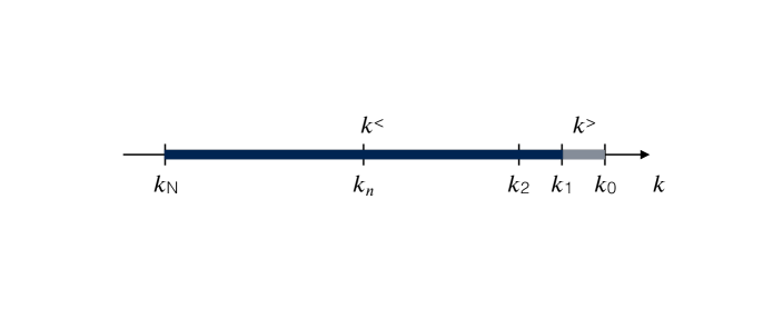
Figure 3: The wavenumber shells to be averaged during renormalization procedure.

In the following subsection we will calculate renormalized viscosity using RG procedure.

VII.3 Renormalization of viscosity using self-consistent procedure

In this subsection we compute renormalized viscosity using self-consistent procedure. This work was done by McComb and his group workers McComb (1990, 2014). The renormalization of viscosity is performed from large wavenumber to smaller wavenumbers.

McComb and his group workers took the following form of Kolmogorov’s spectrum for kinetic energy

$$E(k) = K_{Ko}\Pi^{2/3}k^{-5/3},$$ (69)

where $K_{Ko}$ is Kolmogorov’s constant, and $\Pi$ is the total energy flux. The incompressible fluid equations in the Fourier space are

$$\left(-i\omega+\nu k^{2}\right)u_{i}\left(\hat{{k}}\right) = -\frac{i}{2}P_{ijm}^{+}(\mathbf{k})\int_{\hat{{p}}+\hat{{q}}=\hat{{k}}}d\hat{{p}}\left[u_{j}(\hat{{p}})u_{m}(\hat{{q}})\right],$$ (70)

where

$$P_{ijm}^{+}(\mathbf{k}) = k_{j}P_{im}(\mathbf{k})+k_{m}P_{ij}(\mathbf{k}),$$ (71)

Here $\nu$ is viscosity, and $d$ is the space dimensionality.

In this RG procedure the wavenumber range $(k_{N},k_{0})$ is divided logarithmically into $N$ shells. The $n$th shell is $(k_{n},k_{n-1})$ where $k_{n}=h^{n}k_{0}\,\,(h<1)$. In the following discussion, the elimination of the first shell $(k_{1},k_{0})$ is carried out, and modified NS equation is obtained. Then one proceeds iteratively to eliminate higher shells and get a general expression for the modified fluid equation. The renormalization group procedure is as follows:

1. The the spectral space is divided in two parts: 1. the shell $(k_{1},k_{0})=k^{>}$, which is to be eliminated; 2. $(k_{N},k_{1})=k^{<}$, set of modes to be retained. Note that $\nu_{(0)}$ denote the viscosity and resistivity before the elimination of the first shell.

2. Rewrite Eqs. (70) for $k^{<}$ and $k^{>}$. The equations for $u_{i}^{<}(\hat{k})$ and $b_{i}^{<}(\hat{k})$ modes are

   $$\left(-i\omega+\Sigma_{(0)}(k)\right)u_{i}^{<}(\hat{k}) = -\frac{i}{2}P_{ijm}^{+}({\textbf{k}})\int d\hat{p}([u_{j}^{<}(\hat{p})u_{m}^{<}(\hat{k}-\hat{p})]$$ (72)

   $$+2[u_{j}^{<}(\hat{p})u_{m}^{>}(\hat{k}-\hat{p})]+[u_{j}^{>}(\hat{p})u_{m}^{>}(\hat{k}-\hat{p})])$$

   The $\Sigma$s appearing in the equations are usually called the “self-energy” in Quantum field theory language. In the first iteration, $\Sigma_{(0)}=\nu_{(0)}k^{2}$. The equation for $u_{i}^{>}(\hat{k})$ modes can be obtained by interchanging $<$ and $>$ in the above equations.

3. The terms given in the second and third brackets in the Right-hand side of Eqs. (72) are calculated perturbatively. Since we are interested in the statistical properties of $\mathbf{u}$ fluctuations, we perform the usual ensemble average of the system Yakhot and Orszag (1986). It is assumed that $\mathbf{u}^{>}(\hat{k})$ has Gaussian distributions with zero mean, while $\mathbf{u}(\hat{k})$ is unaffected by the averaging process. Hence,

   $$\left\langle u_{i}^{>}(\hat{k})\right\rangle = 0$$ (73)

   $$\left\langle u_{i}^{<}(\hat{k})\right\rangle = u_{i}^{<}(\hat{k})$$ (74)

   and

   $$\left\langle u_{i}^{>}(\hat{p})u_{j}^{>}(\hat{q})\right\rangle = P_{ij}(\mathbf{p})C(\hat{p})\delta(\hat{p}+\hat{q})$$ (75)

   The triple order correlations $\left\langle u_{i}^{>}(\hat{k})u_{j}^{>}(\hat{p})u_{m}^{>}(\hat{q})\right\rangle$ are zero due to Gaussian nature of the fluctuations. Here, $X$ stands for $u$ or $b$. In addition, we also neglect the contribution from the triple nonlinearity $\left\langle u^{<}(\hat{k})u_{j}^{<}(\hat{p})u_{m}^{<}(\hat{q})\right\rangle$, as done in many of the turbulence RG calculations Yakhot and Orszag (1986); McComb (1990). The effects of triple nonlinearity can be included following the scheme of Zhou and Vahala Zhou et al. (1988).

4. To the first order, the second bracketed terms of Eqs. (72) vanish, but the nonvanishing third bracketed terms yield corrections to $\Sigma$s. Refer to Appendix C for details. Eqs. (72) can now be approximated by

   $$\left(-i\omega+\Sigma_{(0)}+\delta\Sigma_{(0)}\right)u_{i}^{<}(\hat{k}) = -\frac{i}{2}P_{ijm}^{+}({\textbf{k}})\int d\hat{p}[u_{j}^{<}(\hat{p})u_{m}^{<}(\hat{k}-\hat{p})]$$ (76)

   with

   $$\delta\Sigma_{(0)}^{uu}(k) = \frac{1}{(d-1)}\int_{\hat{p}+\hat{q}=\hat{k}}^{\Delta}d\hat{p}[S(k,p,q)G(\hat{p})C(\hat{q})]$$ (77)

   where

   $$S(k,p,q)=kp((d-3)z+2z^{3}+(d-1)xy).$$ (78)

   The integral $\Delta$ is to be done over the first shell.

5. The frequency dependence of the correlation function is taken as: $C(k,\omega)=2C(k)\Re(G(k,\omega))$. In other words, the relaxation time-scale of correlation function is assumed to be the same as that of corresponding Green’s function. Since we are interested in the large time-scale behaviour of turbulence, we take the limit $\omega$ going to zero. Under these assumptions, the frequency integration of the above equations yield

   $$\delta\nu_{(0)}(k) = \frac{1}{(d-1)k^{2}}\int_{\textbf{p+q=k}}^{\Delta}\frac{d\mathbf{p}}{(2\pi)^{d}}\frac{S(k,p,q)C(q)}{\nu_{(0)}(p)p^{2}+\nu_{(0)}(q)q^{2}}$$ (79)

   Note that $\nu(k)=\Sigma^{uu}(k)/k^{2}$ . There are some important points to remember in the above step. The frequency integral in the above is done using contour integral. It can be shown that the integrals are nonzero only when both the components appearing the denominator are of the same sign. For example, first term of Eq. (79) is nonzero only when both $\nu_{(0)}(p)$ and $\nu_{(0)}(q)$ are of the same sign.

6. Let us denote $\nu_{(1)}(k)$ as the renormalized viscosity after the first step of wavenumber elimination. Hence,

   $$\nu_{(1)}(k) = \nu_{(0)}(k)+\delta\nu_{(0)}(k);$$ (80)

   We keep eliminating the shells one after the other by the above procedure. After $n+1$ iterations we obtain

   $$\nu_{(n+1)}(k)=\nu_{(n)}(k)+\delta\nu_{(n)}(k)$$ (81)

   where the equation for $\delta\nu_{(n)}(k)$ is the same as the Eqs. (79) except that $\nu_{(0)}(k)$ appearing in the equation is to be replaced by $\nu_{(n)}(k)$. Clearly $\nu_{(n+1)}(k)$ is the renormalized viscosity and resistivity after the elimination of the $(n+1)$th shell.

7. We need to compute $\delta\nu_{(n)}$ for various $n$. These computations, however, require $\nu_{(n)}$. In our scheme we solve these equations iteratively. In Eqs. (79, LABEL:eq:delta-eta) we substitute $C(k)$ by one dimensional energy spectrum $E(k)$

   $$C(k)=\frac{2(2\pi)^{d}}{S_{d}(d-1)}k^{-(d-1)}E(k)$$

   where $S_{d}$ is the surface area of $d$-dimensional spheres. We assume that $E(k)$ follows Eqs. (69) . Regarding $\nu_{(n)}$, we attempt the following form of solution

   $$\nu_{(n)}(k_{n}k^{\prime})=(K_{Ko})^{1/2}\Pi^{1/3}k_{n}^{-4/3}\nu_{(n)}^{*}(k^{\prime})$$

   with $k=k_{n+1}k^{\prime}\,(k^{\prime}<1)$. We expect $\nu_{(n)}^{*}(k^{\prime})$ to be a universal functions for large $n$. The substitution of $C(k),\nu_{(n)}(k)$ yields the following equations:

   $$\delta\nu_{(n)}^{*}(k^{\prime}) = \frac{1}{(d-1)}\int_{\textbf{p'+q'=k'}}d\mathbf{q}^{\prime}\frac{2}{(d-1)S_{d}}\frac{E^{u}(q^{\prime})}{q^{\prime d-1}}[S(k^{\prime},p^{\prime},q^{\prime})\frac{1}{\nu_{(n)}^{*}(hp^{\prime})p^{\prime 2}+\nu_{(n)}^{*}(hq^{\prime})q^{\prime 2}}]$$ (82)

   $$\nu_{(n+1)}^{*}(k^{\prime}) = h^{4/3}\nu_{(n)}^{*}(hk^{\prime})+h^{-4/3}\delta\nu_{(n)}^{*}(k^{\prime})$$ (83)

   where the integrals in the above equations are performed iteratively over a region $1\leq p^{\prime},q^{\prime}\leq 1/h$ with the constraint that $\mathbf{p}^{\prime}+\mathbf{q}^{\prime}=\mathbf{k}^{\prime}$. Fournier and Frisch Fournier and Frisch (1978) showed the above volume integral in $d$ dimension to be

   $$\int_{\mathbf{p}^{\prime}+\mathbf{q}^{\prime}=\mathbf{k}^{\prime}}d\mathbf{p^{\prime}}=S_{d-1}\int dp^{\prime}dq^{\prime}\left(\frac{p^{\prime}q^{\prime}}{k^{\prime}}\right)^{d-2}\left(\sin\alpha\right)^{d-3},$$ (84)

   where $\alpha$ is the angle between vectors $\mathbf{p}^{\prime}$ and $\mathbf{q}^{\prime}$.

8. Now the above equations are solved self-consistently with $h=0.7$. This value is about middle of the range (0.55-0.75) estimated to be the reasonable values of $h$ by Zhou et al. Zhou et al. (1997). One starts with constant value of $\nu_{(0)}^{*}$, and compute the integrals using Gauss quadrature technique. Once $\delta\nu_{(0)}^{*}$ has been computed, $\nu_{(1)}^{*}$ is computed. This process is iterated till $\nu_{(m+1)}^{*}(k^{\prime})\approx\nu_{(m)}^{*}(k^{\prime})$, that is, till they converge. The result of our RG analysis is given below.

McComb and coworkers McComb (1990); McComb and Watt (1992); Zhou et al. (1997) successfully applied the above self-consistent renormalization group theory to 2D and 3D fluid turbulence. They found that $\nu^{*}(k^{\prime})$ converges quite quickly. For 3D the value of $\nu^{*}(k^{\prime}\rightarrow 0)$ is approximately 0.38. See Fig. 4 for an illustration.

For 2D turbulence $\nu^{*}(k^{\prime})$ is negative as shown in Fig. 4. The function $\nu^{*}$ is not very well behaved as $k^{\prime}\rightarrow 0$. Still, negative renormalized viscosity is consistent with negative eddy viscosity obtained using Test Field Model Kraichnan (1971) and EDQNM calculations Pouquet (1978). We estimate $\nu^{*}\approx-0.60$.

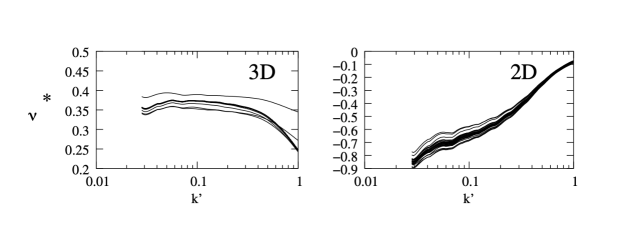
Figure 4: Plot of $\nu^{*}(k^{\prime})$ vs. $k^{\prime}$ for 2D and 3D fluid turbulence. In 2D, $\nu^{*}$ is negative.

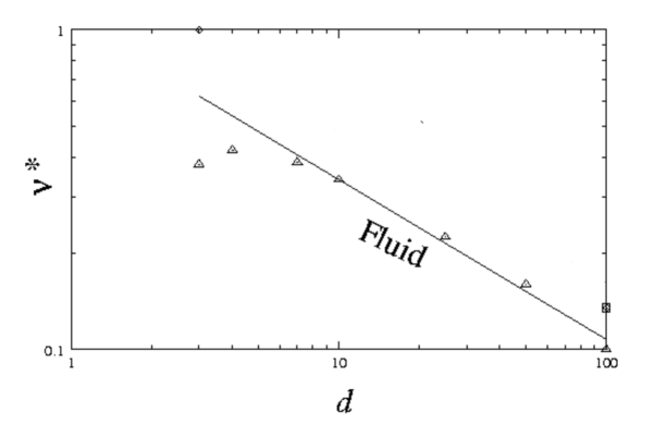
Figure 5: The plot of asymptotic $\nu^{*}$vs. $d$ . For large $d$, the plot fits quite well with predicted $d^{-1/2}$ curve. Adopted from Verma Verma (2004).

For large $d$ , $\nu^{*}=\eta^{*}$, and it decreases as $d^{-1/2}$ (see Fig. 5). $\nu^{*}$ for pure fluid turbulence also decreases as $d^{-1/2}$, as shown in the same figure. This is evident from Eqs. (82) Fournier and Frisch (1978). For large $d$

$$\int dp^{\prime}dq^{\prime}\left(\frac{p^{\prime}q^{\prime}}{k^{\prime}}\right)^{d-2}\left(\sin\alpha\right)^{d-3}... \sim d^{-1/2},$$ (85)

$$\frac{S_{d-1}}{\left(d-1\right)^{2}S_{d}} \sim \frac{1}{d^{2}}\left(\frac{d}{2\pi}\right)^{1/2},$$

$$S,-S_{6},-S_{8},S_{9}(k^{\prime},p^{\prime},q^{\prime}) = kpd(z+xy),$$ (86)

which leads to

$$\nu^{*}\delta\nu^{*}\propto\frac{1}{d^{2}}\left(\frac{d}{2\pi}\right)^{1/2}d^{-1/2}d$$

hence $\nu^{*}\propto d^{-1/2}$.

In conclusion the above RG procedure shows that

$$E(k) = K_{Ko}\Pi^{2/3}k^{-5/3},$$ (87)

$$\nu(k=k_{n}k^{\prime}) = K_{Ko}^{1/2}\Pi^{1/3}k_{n}^{-4/3}\nu^{*}(k^{\prime}),$$ (88)

is a consistent solution of renormalization group equation. Here, $K_{Ko}$ is Kolmogorov’s constant, $\Pi$ is the energy flux, and $\nu^{*}(k^{\prime})$ is a universal function that is a constant as $k^{\prime}\rightarrow 0$.

VII.3.1 Helical turbulence

Helical turbulence is defined for space dimension $d=3$. We can extend the above the RG analysis to helical turbulence (Zhou Zhou et al. (1988); Avinash et al. (2006); Verma (2019)). All the steps are the same except Eqs. (75) are replaced by

$$\left\langle u_{i}^{>}(\hat{p})u_{j}^{>}(\hat{q})\right\rangle = \left[P_{ij}({\textbf{p)}}C^{uu}(\hat{p})-i\epsilon_{ijl}\frac{p_{l}}{p^{2}}H_{K}(\hat{p})\right](2\pi)^{4}\delta(\hat{p}+\hat{q})$$ (89)

Because of helicities, the equation for change in renormalized self-energy (79) gets altered to

$$\delta\nu_{(0)}(k) = \frac{1}{(d-1)k^{2}}\int_{\textbf{p+q=k}}^{\Delta}\frac{d{\textbf{p}}}{(2\pi)^{d}}[\frac{S(k,p,q)C^{uu}(q)+S^{\prime}(k,p,q)H_{K}(q)}{\nu_{(0)}(p)p^{2}+\nu_{(0)}(q)q^{2}}$$

where $S^{\prime}_{i}$ defined below can be shown to be zero.

$$S^{\prime}(k,p,q) = P_{bjm}^{+}(k)P_{mab}^{+}(p)\epsilon_{jal}q_{l}=0,$$

The argument for vanishing of $S^{\prime}$ is follows. Since $\delta\nu$ is a proper scalar, and $H_{K}$ is a pseudo scalar, $S^{\prime}(k,p,q)$ will be also be a pseudo scalar. In addition, $S^{\prime}(k,p,q)$ are also linear in $k,p$ and $q$. This implies that $S^{\prime}_{i}(k,p,q)$ must be proportional to $\mathbf{q}\cdot(\mathbf{k}\times\mathbf{p})$, which will be zero because $\mathbf{k}=\mathbf{p}+\mathbf{q}$. Hence $S^{\prime}(k,p,q)$ turn out to be zero. Hence, helicities do not alter the already calculated $\delta(\nu)_{(n)}(k)$ in the earlier section.

In fluid turbulence, there are some other interesting variations of field-theoretic calculations by DeDominicis and Martin DeDominicis and Martin (1979), Bhattacharjee Bhattacharjee (1991), Carati Carati (1990) and others.

In the next section we will compute energy fluxes for fluid turbulence using field-theoretic techniques.

VIII Field-theoretic Calculation of Energy Fluxes and Shell-to-shell Energy Transfer

In this section we present calculation of energy flux using field-theoretic method. We assume the turbulence to be homogeneous and isotropic. Even though the real-world turbulence do not satisfy these properties, many conclusions drawn using these assumption provide us with important insights into the energy transfer mechanisms at small scales. The field-theoretic procedure requires Fourier space integrations of functions involving products of energy spectrum and the Greens functions. Since there is a general agreement on Kolmogorov-like spectrum for fluid turbulence, $E(k)\propto k^{-5/3}$ is taken for the energy spectrum. For the Greens function, we substitute the “renormalized” or “dressed” Greens function computed in the previous section Verma (2001b) (see Section VII.3).

Most of these works are based on perturbative expansion to first order. We assume that the Fourier modes are quasi-Gaussian that yield the following to first order in perturbation:

$$\Pi_{u}(k_{0}) = \sum_{p\leq k_{0}}\sum_{k>k_{0}}\Im\left[\left\langle{\bf\{k\cdot u(q)\}\{u(p)\cdot u^{*}(k)\}}\right\rangle\right]$$ (90)

$$\sim \sum_{p\leq k_{0}}\sum_{k>k_{0}}\int_{0}^{t}dt^{\prime}G({\bf k},t-t^{\prime})\left\langle{\bf u(p},t)\cdot{\bf u(-p},t^{\prime})\right\rangle\left\langle{\bf u(q},t)\cdot{\bf u(-q},t^{\prime})\right\rangle$$

$$= \Pi_{u}=\mathrm{const},$$

where $G({\bf k},t-t^{\prime})$ is the Green’s function, and $t,t^{\prime}$ are two different times. The quasi-Gaussian nature of the modes yields $\left\langle uuu\right\rangle\sim\left\langle uu\right\rangle\left\langle uu\right\rangle$. The above integral converges and yields a constant. Some of the details of calculations are given below.

VIII.1 Calculation of Energy Flux

As described in Section III the energy flux from a wavenumber sphere of radius $k_{0}$ to the outside of the sphere of the same radius is

$$\Pi(k_{0}) = \frac{1}{(2\pi)^{d}\delta(\mathbf{k^{\prime}+p+q})}\int_{k^{\prime}>k_{0}}\frac{d\mathbf{k^{\prime}}}{(2\pi)^{d}}\int_{p<k_{0}}\frac{d\mathbf{p}}{(2\pi)^{d}}\left\langle S^{uu}(\mathbf{k^{\prime}|p|q})\right\rangle$$ (91)

We assume that the kinetic energy is forced at small wavenumbers.

We analytically calculate the above energy fluxes in the inertial range to leading order in perturbation series. It was assumed that $\mathbf{u}(\mathbf{k})$ is quasi-Gaussian as in EDQNM approximation. Under this approximation, the triple correlation $\left\langle XXX\right\rangle$ is zero to zeroth order, but nonzero to first oder. To first order $\left\langle XXX\right\rangle$ is written in terms of $\left\langle XXXX\right\rangle$, which is replaced by its Gaussian value, a sum of products of second-order moment. Consequently, the ensemble average of $S$, $\left\langle S\right\rangle$, is zero to the zeroth order, but is nonzero to the first order. The first order terms for $\left\langle S(k|p|q)\right\rangle$ in terms of Feynman diagrams are given in Appendix C. They are given below in terms of Green’s functions and correlation functions:

$$\left\langle S(k|p|q)\right\rangle = \int_{-\infty}^{t}dt^{\prime}(2\pi)^{d}[T_{1}(k,p,q)G(k,t-t^{\prime})C(p,t,t^{\prime})C(q,t,t^{\prime})$$ (92)

$$\hskip 28.45274pt+T_{2}(k,p,q)G(p,t-t^{\prime})C(k,t,t^{\prime})C(q,t,t^{\prime})$$

$$\hskip 28.45274pt+T_{3}(k,p,q)G(q,t-t^{\prime})C(k,t,t^{\prime})C(p,t,t^{\prime})]\delta(\mathbf{k^{\prime}}+\mathbf{p}+\mathbf{q})$$

where $T_{i}(k,p,q)$ are functions of wavevectors $k,p$, and $q$ given in Appendix B.

The Greens functions can be written in terms of “effective” or “renormalized” viscosity $\nu(k)$ and resistivity $\eta(k)$ computed in Section VII

$$G(k,t-t^{\prime})=\theta{(t-t^{\prime})}\exp\left(-\nu(k)k^{2}(t-t^{\prime})\right)$$

The relaxation time for $C(k,t,t^{\prime})$ is assumed to be the same as that of $G(k,t,t^{\prime})$. Therefore the time dependence of the unequal-time correlation functions will be

$$C^{uu}(k,t,t^{\prime})=\theta{(t-t^{\prime})}\exp\left(-\nu(k)k^{2}(t-t^{\prime})\right)C^{uu,bb}(k,t,t)$$

The above forms of Green’s and correlation functions are substituted in the expression of $\left\langle S\right\rangle$, and the $t^{\prime}$ integral is performed. Now Eq. (91) yields the following flux formula for $\Pi(k_{0})$:

$$\Pi(k_{0}) = \int_{k>k_{0}}\frac{d\mathbf{k}}{(2\pi)^{d}}\int_{p<k_{0}}\frac{d\mathbf{k}}{(2\pi)^{d}}\frac{1}{\nu(k)k^{2}+\nu(p)p^{2}+\nu(q)q^{2}}\times[T_{1}(k,p,q)C^{uu}(p)C^{uu}(q)$$ (93)

$$\hskip 85.35826pt+T_{2}(k,p,q)C^{uu}(k)C^{uu}(q)+T_{3}(k,p,q)C^{uu}(k)C^{uu}(p)].$$

The expressions for the other fluxes can be obtained similarly.

The equal-time correlation function $C(k,t,t)$ at the steady-state can be written in terms of one dimensional energy spectrum as

$$C(k,t,t)=\frac{2(2\pi)^{d}}{S_{d}(d-1)}k^{-(d-1)}E(k),$$

where $S_{d}$ is the surface area of $d$-dimensional unit spheres. We are interested in the fluxes in the inertial range. Therefore, we substitute Kolmogorov’s spectrum [Eqs.(69)] for the energy spectrum. The effective viscosity is proportional to $k^{-4/3}$, i.e.,

$$\nu(k)=(K^{u})^{1/2}\Pi^{1/3}k^{-4/3}\nu^{*},$$ (94)

and the parameter $\nu^{*}$ was calculated in Section VII.

We nondimensionalize Eq. (93) by substituting Leslie (1973)

$$k=\frac{k_{0}}{u};\,\,\,\,\,p=\frac{k_{0}}{u}v;\,\,\,\,\,q=\frac{k_{0}}{u}w.$$ (95)

Application of Eq. (84) yields

$$\Pi=(K_{Ko})^{3/2}\Pi\left[\frac{4S_{d-1}}{(d-1)^{2}S_{d}}\int_{0}^{1}dv\ln{(1/v)}\int_{1-v}^{1+v}dw(vw)^{d-2}(\sin\alpha)^{d-3}F(v,w)\right],$$ (96)

where the integral $F(v,w)$ are

$$F = \frac{1}{\nu^{*}(1+v^{2/3}+w^{2/3})}[t_{1}(v,w)(vw)^{-d-\frac{2}{3}}+t_{2}(v,w)w^{-d-\frac{2}{3}}+t_{3}(v,w)v^{-d-\frac{2}{3}}],$$ (97)

Here $t_{i}(v,w)=T_{i}(k,kv,kw)/k^{2}$. Note that the energy fluxes are constant, consistent with the Kolmogorov’s picture. We compute the bracketed term (denoted by $I$) numerically using Gaussian-quadrature method, and found it to be convergent. Using $I$ the constant $K_{Ko}$ can be calculated as

$$K_{Ko}=(I)^{-2/3}.$$ (98)

For 3D turbulence, the value of constant $K_{Ko}$ computed using Eqs. (96, 98) is 1.58. This number is very good agreement with numerical and experimental estimate of Kolmogorov’s constant. For 2D turbulence, we substitute $\nu^{*}=-0.60$ in the above equations. The computation yields $K_{Ko}^{2D}\approx 6.3$.

For large $d$

$$\int dp^{\prime}dq^{\prime}\left(\frac{p^{\prime}q^{\prime}}{k^{\prime}}\right)^{d-2}\left(\sin\alpha\right)^{d-3}... \sim d^{-1/2},$$ (99)

$$\frac{S_{d-1}}{\left(d-1\right)^{2}S_{d}} \sim \frac{1}{d^{2}}\left(\frac{d}{2\pi}\right)^{1/2},$$

$$\nu^{*}=\eta^{*} \sim d^{-1/2}$$ (100)

$$t_{1}=-t_{2} = kpd(z+xy),$$ (101)

and $t_{3}=0$. Using Eq. (101) and by matching the dimensions, it can be shown that $K\propto d^{-1/3}$. This result is due to Fournier et al. Fournier and Frisch (1978).

All the above conclusions are for large Reynolds number or $\nu\rightarrow 0$ limit. The behaviour of Navier-Stokes equation for viscosity $\nu=0$ (inviscid) is very different, and has been analyzed using absolute equilibrium theory (see Section IV.2). It can be shown using this theory that under steady state, energy is equipartitioned among all the modes, hence $C(k)=const$ Orszag (1973). Using this result we can compute mode-to-mode energy transfer rates $\left\langle S^{uu}(k|p|q)\right\rangle$ to first order in perturbation theory (Eq. [92]), which yields

$$\left\langle S^{uu}(k|p|q)\right\rangle\propto\int\frac{\left(T_{1}(k,p,q)+T_{5}(k,p,q)+T_{9}(k,p,q)\right)Const}{\nu(k)k^{2}+\nu(p)p^{2}+\nu(q)q^{2}}=0$$

because $T_{1}(k,p,q)+T_{5}(k,p,q)+T_{9}(k,p,q)=0$. Hence, under steady-state, their is no energy transfer among Fourier modes in inviscid Navier-Stokes. In other words “principle of detailed balance” holds here. Note that the above result holds for all space dimensions. Contrast this result with the turbulence situation when energy preferentially gets transferred from smaller wavenumber to larger wavenumber. This example contrasts equilibrium and nonequilibrium systems.

After completing the discussion on energy fluxes for fluid turbulence, we now move on to theoretical computation of shell-to-shell energy transfer.

VIII.2 Field-theoretic Calculation of Shell-to-shell Energy Transfer

Energy transfers between wavenumber shells provide us with important insights into the dynamics of turbulence. Kolmogorov’s fluid turbulence model is based on local energy transfer between wavenumber shells. There are several quantitative theories in fluid turbulence about the amount of energy transfer between neighbouring wavenumber shells. For examples, Kraichnan Kraichnan (1971) showed that $35$% of the energy transfer comes from wavenumber triads where the smallest wave-number is greater than one-half of the middle wavenumber.

In this subsection we will compute the shell-to-shell energy transfer in turbulence using field-theoretic method Verma et al. (2005). The procedure is identical to the one described for energy fluxes. Recall that the energy transfer rates from the $m$-th shell to the $n$-th shell is

$$T_{nm}=\sum_{\mathbf{k^{\prime}}\in n}\sum_{\mathbf{p}\in m}S^{uu}(\mathbf{k^{\prime}|p|q}).$$ (102)

The $\mathbf{p}$-sum is over $m$-th shell, and the $\mathbf{k^{\prime}}$-sum is over $n$-th shell (Section III). The terms of $S$’s are the same as in flux calculation, however, the limits of the integrals are different. The shells are binned logarithmically with $n$-th shell being $(k_{0}s^{n-1},k_{0}s^{n})$. We nondimensionalize the equations using the transformation Leslie (1973)

$$k=\frac{a}{u};\hskip 28.45274ptp=\frac{a}{u}v;\hskip 28.45274ptq=\frac{a}{u}w,$$ (103)

where $a=k_{0}s^{n-1}$. The resulting equation is

$$\frac{T_{nm}}{\Pi}=K_{Ko}^{3/2}\frac{4S_{d-1}}{(d-1)^{2}S_{d}}\int_{s^{-1}}^{1}\frac{du}{u}\int_{us^{m-n}}^{us^{m-n+1}}dv\int_{|1-v|}^{1+v}dw\left(vw\right)^{d-2}\left(\sin{\alpha}\right)^{d-3}F(v,w),$$ (104)

where$F(v,w)$ was computed in the previous section. The renormalized parameters $\nu^{*}$, and Kolmogorov’s constant $K_{Ko}$ required to compute $T_{nm}/\Pi$ are taken from the previous calculations. From Eq. (104) we can draw the following inferences:

1. The shell-to-shell energy transfer rate is a function of $n-m$, that is, $\Phi_{nm}=\Phi_{(n-i)(m-i)}$. Hence, the turbulent energy transfer rates in the inertial range are all self-similar. Of course, this is true only in the inertial range.

2. $T_{nn}/\Pi=0$.

We compute the integral of Eq. (104) and substitute the value of $K_{Ko}$, which yields $T_{nm}$. The plots of $T_{nm}$for 2D and 3D fluids are shown in Fig. 6. In 3D the energy transfer is forward and local. In 2D however the energy transfer is forward for the nearest neighbours, but it is backward for fourth neighbour onward; these backward transfers are one of the major factors in the inverse cascade of energy Verma et al. (2005). The sum of all these transfers is negative energy flux, consistent with the inverse cascade result of Kraichnan Kraichnan (1971). For details refer to Verma et al. Verma et al. (2005).

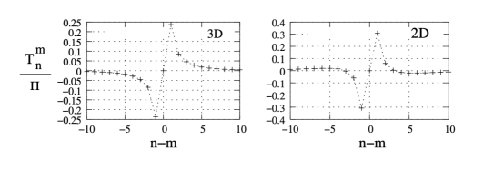
Figure 6: Plots of shell-to-shell energy transfer rates $T_{nm}/\Pi$ vs. $n-m$ for 3D and 2D fluid turbulence.

Verma et al. Verma et al. (2005) computed the shell-to-shell energy transfer in 3D fluid turbulence using numerical simulations. Their result is shown in Fig. 7.

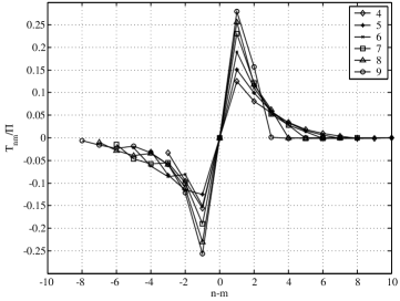
Figure 7: Plot of normalized shell-to-shell energy transfer $T_{nm}/\Pi$ vs. $n-m$ for $d=3$obtained from numerical simulations on $512^{3}$DNS. The $n$th shell is $(k_{0}s^{n}:k_{0}s^{n+1})$ with $s=2^{1/4}.$The energy transfer is maximum for $n=m\pm 1$, hence the energy transfer is local and self-similar. The energy transfer is also forward. Taken from Verma et al. Verma et al. (2005).

Comparison of Fig. 6 and Fig. 7 shows that theoretical and numerical computation of shell-to-shell energy transfer are consistent with each other.

Incompressible fluid turbulence is nonlocal in real space due to incompressibility condition. Field-theoretic calculation also reveals that mode-to-mode transfer $S(k|p|q)$ is large when $p\ll k$, but small for $k\sim p\sim q$, hence Navier-Stokes equation is nonlocal in Fourier space too. However, in 3D shell-to-shell energy transfer rate $T_{nm}$ is forward and most significant to the next-neighbouring shell. Hence, shell-to-shell energy transfer rate is local even though the interactions appear to be nonlocal in both real and Fourier space. Refer to Zhou Zhou (1993), Domaradzki and Rogallo Domaradzki and Rogallo (1990), Verma et al. Verma et al. (2005), and Verma Verma (2005).

With this we conclude our discussion on shell-to-shell energy transfer in hydrodynamic turbulence.

VIII.3 EDQNM Calculation of Fluid Turbulence

Eddy-damped quasi-normal Markovian (EDQNM) calculation of turbulence is very similar to the field-theoretic calculation of energy evolution. This scheme was first invented by Orszag Orszag (1973) for Fluid turbulence.

The Navier-Stokes equation is symbolically written as

$$\left(\frac{d}{dt}+\zeta k^{2}\right)X(\mathbf{k},t)=\sum_{\mathbf{p+q=k}}X(\mathbf{p},t)X(\mathbf{q},t),$$

where $X$ stands for the field u, $X(\mathbf{p},t)X(\mathbf{q},t)$ represents all the nonlinear terms, and $\zeta$ is the dissipation coefficient $(\nu$). The evolution of second and third moment would be

$$\left(\frac{d}{dt}+2\zeta k^{2}\right)\left\langle X(\mathbf{k},t)X(\mathbf{-k},t)\right\rangle = \sum_{\mathbf{p+q=k}}\left\langle X(\mathbf{-k},t)X(\mathbf{p},t)X(\mathbf{q},t)\right\rangle$$ (105)

$$\left(\frac{d}{dt}+\zeta(k^{2}+p^{2}+q^{2})\right)\left\langle X(\mathbf{-k},t)X(\mathbf{p},t)X(\mathbf{q},t)\right\rangle = \sum_{\mathbf{p+q+r+s=0}}\left\langle X(\mathbf{q},t)X(\mathbf{p},t)X(\mathbf{r},t)X(\mathbf{s},t)\right\rangle$$

If $X$ were Gaussian, third-order moment would vanish. However, quasi-normal approximation gives nonzero triple correlation; here we replace $\left\langle XXXX\right\rangle$ by its Gaussian value, which is a sum of products of second-order moments. Hence,

$$\left\langle X(\mathbf{-k},t)X(\mathbf{p},t)X(\mathbf{q},t)\right\rangle = \int_{0}^{t}d\tau\exp{-\zeta(k^{2}+p^{2}+q^{2})(t-\tau)}\sum_{\mathbf{p+q=k}}$$

$$[\left\langle X(\mathbf{q},\tau)X(-\mathbf{q},\tau)\right\rangle\left\langle X(\mathbf{p},\tau)X(\mathbf{p},\tau)\right\rangle+...],$$

where $...$ refers to other products of second-order moments. The substitution of the above in Eq. (105) yields a closed form equation for second-order correlation functions. Orszag Orszag (1973) discovered that the solution of the above equation was plagued by problems like negative energy. To cure this problem, a suitable linear relaxation operator of the triple correlation (denoted by $\mu$) was introduced (Eddy-damped approximation). In addition, it was assumed that the characteristic evolution time of $\left\langle XX\right\rangle\left\langle XX\right\rangle$ is larger than $\left(\mu_{kpq}+\nu(k^{2}+p^{2}+q^{2})\right)^{-1}$(Markovian approximation). As a result the following form of energy evolution equation is obtained

$$\left(\frac{d}{dt}+2\zeta k^{2}\right)\left\langle X(\mathbf{k},t)X(\mathbf{-k},t)\right\rangle=\int d\mathbf{p}\theta_{kpq}(t)\sum_{\mathbf{p+q=k}}[\left\langle X(\mathbf{q},t)X(-\mathbf{q},t\right\rangle\left\langle X(\mathbf{p},t)X(-\mathbf{p},t\right\rangle+...],$$ (106)

where

$$\theta_{kpq}(t)=\left(1-\exp{-(\mu_{k}+\mu_{p}+\mu_{q})t}\right)/\left(\mu_{k}+\mu_{p}+\mu_{q}\right)$$

with

$$\mu_{k}=\left(\nu+\eta\right)k^{2}+C_{s}\left(\int_{0}^{k}dq\left(E^{u}(q)\right)q^{2}\right)^{1/2}.$$ (107)

The first and second terms represent viscous and nonlinear eddy-distortion rates respectively. Note that homogeneity and isotropy are assumed in EDQNM analysis too.

The right-hand side of Eq. (106) is very similar to the perturbative expansion of $S^{uu}(k|p|q)$ (under $t\rightarrow\infty$). The term $\mu_{k}$ of Eq. (107) is nothing but the renormalized dissipative parameters. Thus, field-theoretic techniques for turbulence is quite similar to EDQNM calculation. There is a bit of difference however. In field-theory, we typically compute asymptotic energy fluxes in the inertial range. On the contrary, energy is numerically evolved in EDQNM calculations.

IX Energy flux in real space; Kolmogorov’s four-fifth law (K41)

In this section, we briefly describe the kinetic energy flux in real space. The kinetic energy flows from one scale to next and to next, $l\rightarrow l/2\rightarrow l/4...$, till the dissipation scales where the energy gets dissipated. Our focus is on the formulation by Kolmogorov (1941c, b), who connected the third-order structure function to the energy flux. For the quantification of correlation and structure functions, we consider two real space points, ${\bf r}$ and ${\bf r+l}$, where the velocity fields are ${\bf u(r)}$ and ${\bf u(r+l)}$ respectively. It is convenient to denote ${\bf r+l}$, $u_{i}({\bf r})$, $u_{i}({\bf r+l})$, $\partial/\partial x_{i}$, $\partial/\partial x_{i}^{\prime}$ using ${\bf r^{\prime}}$, $u_{i}$, $u_{i}^{\prime}$, $\partial_{i}$, $\partial_{i}^{\prime}$ respectively. See Fig. 8 for an illustration.

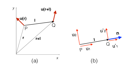
Figure 8: (a) The velocity fields at the two points P and Q are ${\bf u(r)}$ and ${\bf u(r+l)}$ respectively. (b) The components of velocity fields along ${\bf l}$ are $u_{1}$ and $u_{1}^{\prime}$, while the perpendicular components are $u_{2}$, $u_{3}$, $u_{2}^{\prime}$, and $u_{3}^{\prime}$. Here ${\bf n=l}/l$ is the unit vector along ${\bf l}$.

Kolmogorov considered statistically homogeneous, isotropic, and steady turbulence, with forcing employed at large scales. In such flows, the second-order correlation function for the velocity field is  Kolmogorov (1941c); Batchelor (1953)

$$\left\langle u_{i}({\bf r},t)u_{j}({\bf r+l},t)\right\rangle=\left\langle u_{i}u^{\prime}_{j}\right\rangle=C_{ij}(l).$$ (108)

where $u_{i},u_{j}$ are the velocity components, $t$ is time, and $\left\langle.\right\rangle$ represents ensemble average. Note that $C_{ij}(l)$ is a function of $l$ or $|{\bf l}|$, and it is independent of ${\bf r}$, $t$, and orientation of ${\bf l}$. Also, the above correlation is for equal time. Similarly, the third-order longitudinal structure function $S_{3}(l)$ is defined as

$$S_{3}(l)=\left\langle[{\bf(u^{\prime}-u)}\cdot\hat{l}]^{3}\right\rangle,$$ (109)

where $\hat{l}$ is the unit vector along vector ${\bf l}$.

Starting from Navier-Stokes equation, under the assumption of homogeneity and isotropy, Kolmogorov (1941b) derived the following evolution equation for $\left\langle u_{i}u^{\prime}_{j}\right\rangle$:

$$\frac{\partial}{\partial t}\frac{1}{2}\left\langle u_{i}u_{i}^{\prime}\right\rangle = \frac{1}{2}\left\langle u_{i}^{\prime}\frac{\partial}{\partial t}u_{i}\right\rangle+\frac{1}{2}\left\langle u_{i}\frac{\partial}{\partial t}u_{i}^{\prime}\right\rangle$$ (110)

$$= \frac{1}{2}\left[-\partial_{j}\left\langle u_{i}^{\prime}(u_{j}u_{i})\right\rangle-\partial_{j}^{\prime}\left\langle u_{i}(u_{j}^{\prime}u_{i}^{\prime})\right\rangle-\cancel{\partial_{i}\left\langle pu_{i}^{\prime}\right\rangle}-\cancel{\partial_{i}^{\prime}\left\langle p^{\prime}u_{i}\right\rangle}\right.$$

$$\left.+\left\langle u_{i}^{\prime}F_{\mathrm{LS},i}\right\rangle+\left\langle u_{i}F_{\mathrm{LS},i}^{\prime}\right\rangle+\nu\left\langle u_{i}^{\prime}\nabla^{2}u_{i}\right\rangle+\nu\left\langle u_{i}\nabla^{\prime 2}u_{i}^{\prime}\right\rangle\right]$$

$$= \frac{1}{2}\left[\partial_{j}^{\prime}\left\langle u_{i}^{\prime}(u_{j}u_{i})\right\rangle-\partial_{j}^{\prime}\left\langle u_{i}(u_{j}^{\prime}u_{i}^{\prime})\right\rangle+2\left\langle u_{i}^{\prime}F_{\mathrm{LS},i}\right\rangle+2\nu\nabla^{\prime 2}\left\langle u_{i}u_{i}^{\prime}\right\rangle\right]$$

$$= \frac{1}{4}\nabla_{l}\cdot\left\langle|{\bf u^{\prime}-u}|^{2}({\bf u^{\prime}-u})\right\rangle+\left\langle F_{\mathrm{LS},i}u_{i}^{\prime}\right\rangle+\nu\nabla^{\prime 2}\left\langle u_{i}u_{i}^{\prime}\right\rangle$$

$$= T_{u}({\bf l})+\mathcal{F}_{\mathrm{LS}}({\bf l})-D_{u}({\bf l}).$$

The above derivation makes use of tensorial and symmetry properties (homogeneity and isotropy) of the correlation functions. For example, $\left\langle pu^{\prime}_{i}\right\rangle=\left\langle p^{\prime}u_{i}\right\rangle=0$ due to isotropy. For details, refer to Kolmogorov (1941b); Landau and Lifshitz (1987); Frisch (1995); Brachet (2000).

In Eq. (110), $T_{u}({\bf l})$ corresponds to the spectral energy transfer term $T_{u}({\bf k})$; and $\mathcal{F}_{u}({\bf l})$ and $D_{u}({\bf l})$ are the respective correlations of the energy injection rate and the dissipation rate. Further, Kolmogorov Kolmogorov (1941b) assumed the following:

1. $\partial\left\langle u_{i}u_{i}^{\prime}\right\rangle/\partial t=0$ due to the steady nature of the flow.

2. $\nu\rightarrow 0$, hence the dissipation wavenumber ($k_{d}$) is at infinity.

3. The flow is forced at large scales, hence $\mathcal{F}_{\mathrm{LS}}(l)\approx\epsilon_{u}$, and it is approximately the same at all scales.

In addition, we focus on the inertial range, $1/k_{d}\ll l\ll L$, where the viscous dissipation $D_{u}({\bf l})=2\nu\nabla^{\prime 2}\left\langle u_{i}u_{i}^{\prime}\right\rangle\rightarrow 0$. Therefore, Eq. (110) yields

$$\mathcal{F}_{\mathrm{LS}}(l)\approx\epsilon_{u}\approx-T_{u}(l)=-\frac{1}{4}\nabla_{l}\cdot\left\langle|{\bf u^{\prime}-u}|^{2}({\bf u^{\prime}-u})\right\rangle.$$ (111)

We denote

$${\bf Q(l)} = \left\langle|{\bf u^{\prime}-u}|^{2}({\bf u^{\prime}-u})\right\rangle,$$ (112)

$$\bar{S}_{3}(l) = \left\langle|{\bf u^{\prime}-u}|^{2}\{({\bf u^{\prime}-u})\cdot\hat{l}\}\right\rangle.$$ (113)

Since ${\bf Q(l)}$ is a isotropic vector, we deduce that

$${\bf Q(l)}=\bar{S}_{3}(l)\hat{l},$$ (114)

whose substitution in Eq. (111) yields the following equation (in spherical coordinate system for ${\bf l}$):

$$-\frac{1}{4}\frac{1}{l^{2}}\frac{d}{dl}\left[l^{2}\bar{S}_{3}(l)\right]=\epsilon_{u}.$$ (115)

The solution of the above equation is

$$\bar{S}_{3}(l)=-\frac{4}{3}\epsilon_{u}l,$$ (116)

which is the four-third law.

It is easy to show that  Kolmogorov (1941b); Frisch (1995)

$$\bar{S}_{3}(l)=\frac{1}{3}\left[l\frac{d}{dl}S_{3}(k)+4S_{3}(l)\right]=\frac{1}{3l^{3}}\frac{d}{dl}\left[l^{4}S_{3}(k)\right].$$ (117)

Using Eqs. (116, 117), we immediately deduce the third-order longitudinal structure function as

$$S_{3}(l)=\left\langle[{\bf(u^{\prime}-u)}\cdot\hat{l}]^{3}\right\rangle=-\frac{4}{5}\epsilon_{u}l.$$ (118)

This is the Kolmogorov’s four-fifth law, which has been verified in various experiments and simulations Frisch (1995); Davidson (2004). Using Eqs. (116, 118), we deduce the third-order transverse structure function as

$$\left\langle|{\bf u_{\perp}^{\prime}-u_{\perp}}|^{2}({\bf u^{\prime}-u})\right\rangle=-\left(4/3-4/5\right)\epsilon_{u}l=-\frac{8}{15}\epsilon_{u}l,$$ (119)

where ${\bf u}_{\perp}$ is the velocity component perpendicular to ${\bf l}$, and $|{\bf u_{\perp}^{\prime}-u_{\perp}}|^{2}=|{\bf u^{\prime}-u}|^{2}-|({\bf u^{\prime}-u})\cdot\hat{l}|^{2}$. Eyink (2002) derived the above relations earlier.

The prefactors for the longitudinal and transverse structure functions, $4/5$ and $8/15$, are of the same order. This is consistent with the observations of Dhruva et al. (1997) who employed atmospheric turbulence data to deduce that the longitudinal and transverse structure functions are close to each other. Shen and Warhaft (2002) arrived at a similar conclusion based on their studies on sheared and unshared wind-tunnel turbulence.

The aforementioned four-third and four-fifth laws have been derived under the assumption that the external force is applied at the large scales leading to $\mathcal{F}_{\mathrm{LS}}(l)\approx\epsilon_{u}$, a constant. However, we can generalise the above laws to isotropic forcing employed in the inertial range. Suppose that in the inertial range, the correlation function related to energy injection rate is $\mathcal{F}_{u}(l)$, then Eq. (111) translates to

$$\mathcal{F}_{u}(l)=-T_{u}(l)=-\frac{1}{4}\nabla_{l}\cdot\left\langle|{\bf u^{\prime}-u}|^{2}({\bf u^{\prime}-u})\right\rangle.$$ (120)

whose solution is

$$\bar{S}_{3}(l)=-\frac{4}{l^{2}}\int^{l}dl^{\prime}\mathcal{F}_{u}(l^{\prime})l^{\prime 2}.$$ (121)

For $\mathcal{F}_{u}(l)=\epsilon_{u}$, we recover the four-third law.

The above real-space description is closely related to the corresponding Fourier space description. We show below that Eq. (111) is related to its Fourier space equivalent. See Fig. 9 for an illustration. In $-T_{u}(l)$, the product $|{\bf u^{\prime}-u}|^{2}$ includes the giver and receiver fields, while the third $\delta{\bf u}$ is the mediator field. Since the real space $\delta{\bf u}$ is a linear superposition of many Fourier modes, $\Pi_{u}(k)$, which is the complement of $T_{u}(l)$, involves sums over ${\bf p}$ and ${\bf k}$ modes. Also note that $K\leftrightarrow 1/l$ is the radius of the wavenumber sphere.

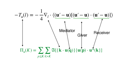
Figure 9: A figure illustrating connections between $-T_{u}(l)$ and the energy flux $\Pi_{u}(K)$. We contrast the receiver, giver, and mediator fields in both the formulas.

Both, the four-fifth law and the variable energy flux equation, $d\Pi_{u}/dk=-\mathcal{F}_{u}(k)$, are exact relations in statistical sense. This is because their derivation is based on conservation of energy. An interesting departure however is isotropy. The Fourier-space definition of flux has been employed to anisotropic system, for example to quasi-static MHD turbulence after angular averaging. However, Kolmogorov’s four-fifth law assumes isotropy, though there have been attempts to generalise it to anisotropic turbulence  Danaila et al. (2012); Ching (2013).

The skewness $S$ for a turbulent flow is defined using

$$\left\langle\left(\frac{\partial u_{1}}{\partial x_{1}}\right)^{2}\right\rangle^{3/2}/\left\langle\left(\frac{\partial u_{1}}{\partial x_{1}}\right)^{3}\right\rangle=\frac{1}{S}.$$ (122)

Kolmogorov (1941b) assumed that

$$\left\langle(\Delta u)_{\parallel}^{2}\right\rangle=\left\langle\frac{1}{S}S_{3}(l)\right\rangle^{2/3}\sim\Pi^{2/3}l^{2/3}.$$ (123)

Using the above it can be deduced that

$$\left\langle{\bf u(r+l)\cdot u(r)}\right\rangle\sim C-\Pi_{u}^{2/3}l^{2/3},$$ (124)

where $C$ is a constant. The Fourier transform of the above correlation yields Kolmogorov’s spectrum, apart from a constant  Batchelor (1953).

A trivial generalisation of the above relations to higher order structure functions yields

$$S_{q}(l)=\left\langle(\Delta u)_{\parallel}^{q}\right\rangle=C_{q}\Pi^{q/3}l^{q/3}\sim l^{\zeta_{q}}$$ (125)

leading to $\zeta_{q}=q/3$, and $C_{q}$ as constants. The exponents $\zeta_{q}$’s are called intermittency exponents. However, contrary to the above predictions, the experiments and numerical simulations reveal that $\zeta_{q}<q/3$, specially for large $q$’s; this is the topic of the next section.

X Beyond K41; Fluctuations in energy flux

In Kolmogorov’s theory of hydrodynamic turbulence, the kinetic energy cascades to intermediate scales and then to smaller scales. In Fourier space, conservation of energy for a shell leads to $\Pi_{u}(k)=\mathrm{const}$ in the inertial range. However, this theory does not provide information about the distribution of energy among the daughter eddies. An uneven distribution of the energy flux among the daughter eddies leads to fluctuations in the flux, whose quantification is the topic of the present section.

Landau and Lifshitz (1987) pointed out that the viscous dissipation ($\nu\omega^{2}$) in a turbulent flow is singular. That is, there are tiny regions of strong viscous dissipation in a sea where the average dissipation is weak. The above phenomenon, observed in many experiments and numerical simulations, is due to an uneven distribution of energy flux among the daughter eddies. This distribution has been studied using various models, which will be presented In the following discussion. We refer the reader to Frisch (1995), Dubrulle (2019), and Stolovitzky and Sreenivasan (1994) for details.

X.1 Fractal model

Frisch et al. (1978) and Frisch (1995) constructed a fractal-based model, popularly known as $\beta$ model, for the energy cascade. They assumed fluid structures to be a fractal with a fractal dimension of $D$. Here, the fraction of “active" space in a turbulent cascade decreases as a power law:

$$p_{l}=\beta^{n}=\left(\frac{l}{L}\right)^{(3-D)},$$ (126)

where $l=2^{-n}L$ is the length scale of the eddies at the $n$th level. Hence, the energy flux at length scale $l$ would be

$$\Pi_{l}=\frac{u_{l}^{3}}{l}p_{l}=\frac{u_{l}^{3}}{l}\left(\frac{l}{L}\right)^{(3-D)}.$$ (127)

Constancy of energy flux in the inertial range implies that $\Pi_{l}=\Pi$, i.e.,

$$\Pi_{l}=\frac{U_{L}^{3}}{L}.$$ (128)

This leads to

$$u_{l}=U_{L}\left(\frac{l}{L}\right)^{1/3-(3-D)/3}.$$ (129)

Therefore, in this model, the $q$th-order structure function is

$$S_{q}(l)=\left\langle(\Delta u)_{\parallel}^{q}\right\rangle\sim\left\langle u_{l}^{q}\right\rangle\sim u_{l}^{q}p_{l}\sim U_{L}^{q}\left(\frac{l}{L}\right)^{q[1/3-(3-D)/3]}\left(\frac{l}{L}\right)^{(3-D)}.$$ (130)

The above expression yields the intermittency exponent as

$$\zeta_{q}=\frac{q}{3}+(3-D)\left(1-\frac{q}{3}\right).$$ (131)

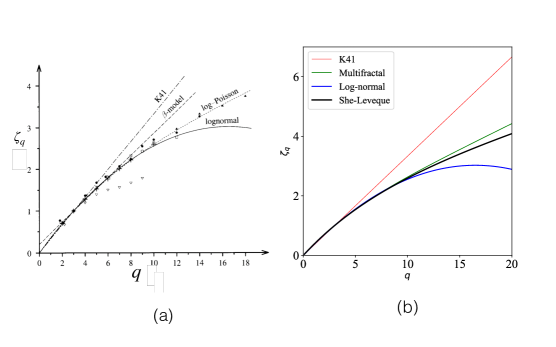
Figure 10: Plots of $\zeta_{q}$ vs. $q$ for various models and those computed using experimental data. The experimental results Anselmet et al. (1984) are shown as triangles and circles. The plot of $\beta$-model is constructed using $D=2.8$, that of multifractal model using $p=0.7$, and that of log-normal model using $\mu=0.2$. Figure (a) is adopted from a figure of Frisch (1995).

Note that $\zeta_{q}=q/3$ for $D=3$. This situation corresponds to homogeneous dissipation among all the eddies at any scale. Imagine a cube being divided into 8 equal-sized cubes, which are successively cut into 8 cubes each. For $D=3$, each cube at level 1 will receive $\Pi_{u}/8$ units of energy flux, and then they will pass on $\Pi_{u}/64$ units of energy flux to daughter cubes, and so on. Such distribution of $\Pi_{u}$ corresponds to $p_{l}=1$. Now contrast the above with structures with $D<3$. Here, the energy flux is divided as in fractals, e.g., three-dimensional Sierpinski Gasket or Menger sponge  Addison (1997). These structures, as well the energy cascade in them, are self-similar.

In Fig. 10(a) we illustrate a plot of $\zeta_{q}$ vs. $q$ for $D=2.8$. The model predictions match with experimental results of Anselmet et al. (1984) only till $q\approx 8$  Frisch (1995). The above discrepancy is corrected in multifractal models of turbulence.

X.2 Multifractal model

The $\beta$-model of turbulence discussed in the previous subsection assumes the turbulent structures to be a homogeneous fractal. Experimental observations however reveal that the structures are inhomogeneous, that is, the fractal dimension of the turbulent structures varies with position. Hence, researchers have proposed multifractal model of turbulence  Frisch and Parisi (1985); Frisch (1995); Meneveau and Sreenivasan (1987a, b); Addison (1997); Grassberger and Procaccia (1983). In this subsection we illustrate the central idea of multifractality using Meneveau and Sreenivasan (1987a)’s model.

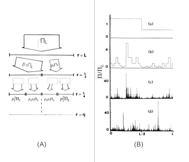
Figure 11: (A) A schematic diagram illustrating distribution of energy flux during a one-dimensional cascade process. In the multifractal model of Meneveau and Sreenivasan (1987a), the two daughter eddies receive fraction $p_{1}$ and $p_{2}=1-p_{1}$ of $\Pi_{l}$. This cascade process is continued successively. (B) The distribution of $\Pi_{l}$ at the (a) first stage, (b) fifth stage, (c) twelfth stage. (d) A distribution of $\Pi_{l}$ in an experimental signal resembles distribution of (c). From Meneveau and Sreenivasan (1987a).

Therefore, the fractal dimension for the three-dimensional structures would be

$$D_{q}=\bar{D}_{q}+2.$$ (132)

Note that $D_{q}$ is function of $q$ due to multifractal nature of the structures. This feature is related to space variability of the fractal dimension  Frisch (1995); Addison (1997); Grassberger and Procaccia (1983). In contrast, for the $\beta$-model, $D_{q}=D$ for all $q$’s due the fractal nature of the flow. The intermittency exponent $\zeta_{q}$ for the above multifractal model can be computed by substituting $D_{q}$ of Eq. (132) in Eq. (131) that yields  Meneveau and Sreenivasan (1987b)

$$\zeta_{q}=\frac{q}{3}+(3-2-\bar{D}_{q/3})\left(1-\frac{q}{3}\right)=\left(\frac{q}{3}-1\right)\bar{D}_{q/3}+1.$$ (133)

We illustrate the above $\zeta_{q}$ in Fig. 10(b). We remark that the deviation of $\zeta_{q}$ from $q/3$ is due to the spatial intermittency of $\Pi_{l}$, hence it is called intermittency correction. Meneveau and Sreenivasan (1987a, b) also computed $\zeta_{q}$ using data from several experiments (grid turbulence, wake of a circular cylinder, atmospheric turbulence). The model $\zeta_{q}$ with $p=0.7$ provides best fit to the experimental results.

X.3 Lognormal model

The multifractal model of Meneveau and Sreenivasan (1987a) is made probabilistic by a modified prescription, according to which the incident energy flux for an arbitrary eddy is  Kolmogorov (1962); Gurvich and Yaglom (1967); Frisch (1995)

$$\Pi_{l}=\eta_{1}\eta_{2}...\eta_{n}\Pi=\Pi\prod_{i}\eta_{i},$$ (134)

where $\eta_{i}$ is a random variable. Since $\Pi_{l}$ is a product of random variables, it follows a lognormal distribution.

$$\log\Pi_{l}=\log\Pi+\sum_{i}\log\eta_{i}$$ (135)

follows a gaussian distribution, or

$$P(\Pi_{l})=\frac{1}{\sigma\Pi_{l}\sqrt{2\pi}}\exp\left(-\frac{(\log\Pi_{l}-M)^{2}}{2\sigma^{2}}\right),$$ (136)

where $M$ and $\sigma$ are respectively the mean and standard deviation of $\Pi_{l}$  Kolmogorov (1962); Gurvich and Yaglom (1967); Frisch (1995).

Using the above probability distribution we deduce that

$$\frac{\left\langle\Pi_{l}^{q}\right\rangle}{\left\langle\Pi_{l}\right\rangle^{q}}=\exp\left(Mq+\frac{1}{2}\sigma^{2}q^{2}\right).$$ (137)

Let us postulate that the above ratio is

$$\frac{\left\langle\Pi_{l}^{q}\right\rangle}{\left\langle\Pi_{l}\right\rangle^{q}}=A_{q}\left(\frac{L}{l}\right)^{\tau_{q}},$$ (138)

where $\tau_{q}$ and $A_{q}$ are constants. The constants $M$ and $\sigma$ are related to each other as follows. By setting $q=1$ in Eq. (137), we obtain $M=-\sigma^{2}/2$. Hence,

$$\frac{\left\langle\Pi_{l}^{q}\right\rangle}{\left\langle\Pi_{l}\right\rangle^{q}}=\exp\left(\frac{1}{2}\sigma^{2}q(q-1)\right).$$ (139)

By definition, substitution of $q=2$ in Eq. (139) yields the variance of $\Pi_{l}$ as

$$\frac{\left\langle\Pi_{l}^{2}\right\rangle}{\left\langle\Pi_{l}\right\rangle^{2}}=\exp(\sigma^{2})\equiv A\left(\frac{L}{l}\right)^{\mu},$$ (140)

or

$$\sigma^{2}=\log A+\mu\log(L/l),$$ (141)

$A_{2}=A$, and $\tau_{2}=\mu$. Substitution of Eq. (140) in Eq. (139) yields

$$\left\langle\Pi_{l}^{q}\right\rangle=A_{q}\left\langle\Pi_{l}\right\rangle^{q}\left(\frac{l}{L}\right)^{-\frac{\mu}{2}q(q-1)},$$ (142)

and hence,

$$\tau_{q}=-\frac{\mu}{2}q(q-1).$$ (143)

Therefore, using Eq. (142) we derive

$$\left\langle(\Delta_{l}u)^{q}\right\rangle = \left\langle\Pi_{l}^{(q/3)}\right\rangle l^{q/3}\approx A_{q/3}\left\langle\Pi\right\rangle^{q/3}l^{\zeta_{q}}L^{-\tau_{q/3}},$$ (144)

where

$$\zeta_{q}=\frac{q}{3}+\tau_{q/3}=\frac{q}{3}-\frac{\mu}{18}q(q-3).$$ (145)

Note that $\zeta_{6}=2-\mu$, a relation that is used to estimate $\mu$. The experiments  Benzi et al. (1993); Frisch (1995) reveal that $\mu\approx 0.22$, albeit with significant errors.

The predictions of lognormal model are illustrated in Fig. 10 for $\mu=0.2$. The model predictions match with the experimental data quite well till $q\approx 12$ (see Fig. 10(a)), but they deviate significantly for larger $q$’s. In the next subsection we present another model that corrects for the above deficiency.

X.4 She Leveque model

The intermittency correction ($q/3-\zeta_{q}$) for the lognormal model is larger than those observed in experiments, especially for large $q$’s. This is because for large $q$, $\left\langle\Pi_{l}^{q}\right\rangle$ is suppressed very strongly due to lognormal nature of $\Pi_{l}$. In particular, for large $q$, Eq. (142) yields

$$\left\langle\Pi_{l}^{q}\right\rangle\sim\left(\frac{l}{L}\right)^{-\frac{\mu}{2}q^{2}}.$$ (146)

She and Leveque (1994) corrected this discrepancy by a very interesting postulate. They argued that asymptotically (for large $q$), singular nature of the vortex filaments is expected to follow

$$\Pi_{l}^{(\infty)}=\frac{\left\langle\Pi_{l}^{(q+1)}\right\rangle}{\left\langle\Pi_{l}^{q}\right\rangle}\sim\left(\frac{l}{L}\right)^{-2/3}.$$ (147)

In other words, for large $q$,

$$\left\langle\Pi_{l}^{q}\right\rangle\sim\left(\frac{l}{L}\right)^{-2q/3},$$ (148)

and hence,

$$\zeta_{q}\approx\frac{q}{3}+\tau_{q/3}\approx\frac{q}{3}-\frac{2q}{9}\approx\frac{q}{9}.$$ (149)

The above prediction appears to match with the experimental observations for $q>12$ where lognormal distribution tends to fail. Note that She and Leveque (1994)’s ansatz allows for presence of larger fluctuations in $\Pi_{l}$; it is also termed as log-Poisson model  Dubrulle (1994); She and Waymire (1995).

To compute $\zeta_{q}$ for all $q$’s, She and Leveque (1994) postulated that

$$\left\langle\Pi_{l}^{(q+1)}\right\rangle=\left\langle\Pi_{l}^{(q)}\right\rangle^{\beta}\left(\Pi_{l}^{(\infty)}\right)^{(1-\beta)}.$$ (150)

The above equation has a solution:

$$\tau_{q}=-\frac{2}{3}q+2\left[1-\left(\frac{2}{3}\right)^{q}\right]$$ (151)

that leads to

$$\zeta_{q}=\frac{q}{9}+2\left[1-\left(\frac{2}{3}\right)^{(q/3)}\right]$$ (152)

The above $\zeta_{q}$ fits with the experimental and numerical results quite well, as illustrated in Fig. 10  She and Leveque (1994); Frisch (1995).

Now let us compare the results of the four models and K41. She-Leveque’s model predicts that $\zeta_{2}\approx 0.696\approx(2/3)+0.03$, thus it deviates from K41 prediction by 0.03. As a result, the energy spectrum is

$$E_{u}(k)\sim\Pi^{2/3}k^{-5/3-0.03}L^{0.03}.$$ (153)

Thus, the energy spectrum and structure function depend on the system size (though weakly), contrary to the assumptions of universal theory of turbulence. Note however that the constancy of energy flux still holds; it is related to the energy conservation and Kolmogorov’s four-fifth law. The deviation from the scale-symmetric exponent $\zeta_{q}=q/3$ is due to the multifractal nature of turbulence  Frisch (1991). See Frisch (1995) for more details on symmetry arguments.

As shown in Fig. 10, the predictions of the four models are quite close to each other for $q=2$ to 5, and those of multifractal, lognormal and She-Leveque’s models match till $q\approx 10$  Frisch (1995). For larger $q$’s, only She-Leveque’s model provides good fit to the experimental results. As described earlier in this section, the deviation from $\zeta_{q}=q/3$ is due to the fact that the turbulent structures are multifractal (not fractal). Singular dissipation at small scales contribute more significantly to the structure functions for large $q$’s.

It is interesting to contrast the distributions of kinetic energy spectrum and flux. The former has a power law behaviour in $l$ or wavenumber $k$, while latter exhibits lognormal or log-Poisson distribution. This difference is essentially due to fact that the energy spectrum is a distribution across various scales. On the contrary, Eq. (136) describes the lognormal distribution of energy flux at a given scale $l$. The latter distribution occurs in a branching process after many iterations. Note that a sum of $\Pi_{l}$ for all the eddies at scale $l$ is a constant (statistically), and it equals the total energy flux $\Pi$.

Branching process is observed in many natural phenomena, for example, in fragmentation, population development, gene propagation, natural growth, etc. Following this idea, the mass distribution in the universe is conjectured to be log-normal Coles and Jones (1991); this distribution can be easily explained using multiscale fragmentation process in the universe. Though cosmic anisotropy is a complex problem, the above simple idea may provide interesting connections between the observed anisotropy and fragmentation caused by the big bang. Similarly, branching process in a tree accounts for the lognormal distribution of length of terminal twigs  Koyama et al. (2017).

XI Structure function for 2D turbulence

In this section, we briefly describe the structure functions of 2D turbulence  Gotoh (1998); Lindborg (1999); Bernard (1999). The situation for 2D turbulence is more complex than for 3D counterpart due to forcing at the intermediate wavenumbers. We inspect the structure functions for $k<k_{f}$ and $k>k_{f}$ regimes that exhibit different scaling. Here we focus only on the inertial range, hence ignore the effects of viscous force and Ekman friction.

For the inertial range in the $k<k_{f}$ regime, the equation for the velocity correlation function is same as Eq. (110). For the correlation function $\mathcal{F}_{u}(l)$, it is assumed that

$$\mathcal{F}_{u}(l)\approx-\epsilon_{u,\alpha}\approx-\epsilon_{u}.$$ (154)

In addition, the dissipation is assumed to negligible in this range. Hence,

$$-\epsilon_{u} = -T_{u}(l)=-\frac{1}{4}\nabla_{l}\cdot\left\langle|{\bf u^{\prime}-u}|^{2}({\bf u^{\prime}-u})\right\rangle.$$ (155)

We denote

$${\bf Q(l)} = \left\langle|{\bf u^{\prime}-u}|^{2}({\bf u^{\prime}-u})\right\rangle,$$ (156)

$${S}_{3}(l) = \left\langle|{\bf u^{\prime}-u}|^{2}\{({\bf u^{\prime}-u})\cdot\hat{l}\}\right\rangle.$$ (157)

Due to the isotropic nature of ${\bf Q(l)}$, we deduce that

$${\bf Q(l)}={S}_{3}(l)\hat{l},$$ (158)

whose substitution in Eq. (155) yields

$$\frac{1}{4}\frac{1}{l}\frac{d}{dl}\left[l{S}_{3}(l)\right]=\epsilon_{u}.$$ (159)

Note that the divergence operator for a 2D radially-symmetric vector field ${\bf Q(l)}=Q_{l}\hat{l}$ is $(1/l)d(lQ_{l})/dl$. Hence, the solution of Eq. (159) is  Lindborg (1999); Bernard (1999)

$${S}_{3}(l)=2\epsilon_{u}l.$$ (160)

Contrast the above relation with Eq. (116) for 3D hydrodynamic turbulence. The opposite sign of Eq. (160) indicates inverse energy cascade for 2D hydrodynamic turbulence.

The above relation was first derived by Lindborg (1999) and Bernard (1999). Further, using the symmetry properties of the tensors, Lindborg (1999) showed that

$$\left\langle[{\bf(u^{\prime}-u)}\cdot\hat{l}]^{3}\right\rangle=\frac{3}{4}{S}_{3}(l).$$ (161)

Therefore,

$$\left\langle[{\bf(u^{\prime}-u)}\cdot\hat{l}]^{3}\right\rangle = \frac{3}{2}\epsilon_{u}l,$$ (162)

$$\left\langle{\bf(u^{\prime}_{\perp}-u_{\perp})}^{2}\{{\bf(u^{\prime}-u)}\cdot\hat{l}\}\right\rangle = \frac{1}{2}\epsilon_{u}l,$$ (163)

where ${\bf u}_{\perp}$ is the velocity component perpendicular to ${\bf l}$. The relation of Eq. (162) has been verified numerically by Boffetta et al. (2000).

In the $k>k_{f}$ regime, the enstrophy flux dominates the energy flux. Hence, the structure function for the vorticity is reported for this regime  Gotoh (1998); Lindborg (1999); Bernard (1999). Following similar arguments as that for passive scalar, one can derive the evolution equation for the vorticity correlation function $\left\langle\omega\omega^{\prime}\right\rangle$ as

$$\frac{\partial}{\partial t}\frac{1}{2}\left\langle\omega\omega^{\prime}\right\rangle = \frac{1}{4}\nabla_{l}\cdot\left\langle|\omega-\omega^{\prime}|^{2}({\bf u^{\prime}-u})\right\rangle+\left\langle F_{\omega}\omega^{\prime}\right\rangle+\nu\nabla^{\prime 2}\left\langle\omega\omega^{\prime}\right\rangle$$ (164)

$$= T_{\omega}({\bf l})+\mathcal{F}_{\omega}({\bf l})-D_{\omega}({\bf l}).$$

Hence, in the inertial range,

$$\left\langle|\omega-\omega^{\prime}|^{2}({\bf u^{\prime}-u})\cdot\hat{l}\right\rangle=-2\epsilon_{\omega}l,$$ (165)

where $\epsilon_{\omega}$ is the enstrophy dissipation rate. Further, Lindborg (1999) generalised Eq. (164) to

$$\frac{\partial}{\partial t}\frac{1}{2}\left\langle\omega\omega^{\prime}\right\rangle = \frac{1}{4}\nabla_{l}^{2}\nabla_{l}\cdot\left\langle|{\bf u-u^{\prime}}|^{2}({\bf u^{\prime}-u})\right\rangle+\mathcal{F}_{\omega}({\bf l})-D_{\omega}({\bf l}).$$ (166)

From the above equation, it is straightforward to derive that Lindborg (1999)

$$\left\langle|{\bf u^{\prime}-u}|^{2}({\bf u^{\prime}-u})\cdot\hat{l}\right\rangle=-\frac{1}{8}\epsilon_{\omega}l.$$ (167)

Gotoh (1998) started from Eq. (165) and derived that $E_{u}(k)\propto k^{-(3+\delta)}$ for $k<k_{d2D}$, and $E_{u}(k)\propto k^{-(3+\delta)/2}\exp(-\alpha_{2}k/k_{d2D})$ for $k>k_{d2D}$, where $\alpha_{2},\delta$ are constants. Gotoh (1998) also verified the above scaling using numerical simulations.

Regarding the higher order structure function, Boffetta et al. (2000) and Tabeling (2002) argue that in the $k<k_{f}$ regime, $\zeta_{q}\approx q/3$, thus signalling an absence of intermittency in 2D turbulence. These authors also claim that in the inertial range, the probability distribution function of velocity increments is close to gaussian, which is consistent with the non-intermittent nature of the flow. Boffetta and Ecke (2012) however show that longitudinal velocity increment deviates from gaussian distribution. These issues may require further investigation. Using numerical simulations, Babiano and Dubrulle (1995) and Babiano et al. (1997) computed the multiscaling exponents for the $k<k_{f}$ regime of 2D turbulence. Babiano et al. (1997) related the intermittency exponents to the homogeneity and stationarity of the transfers in the inverse energy cascade.

XI.1 Field-theoretic description of energy flux and intermittency

K41 is an analytical theory of turbulence. In addition, there are several field-theoretic calculations of turbulence, which are first-principle treatment of the problem. Field theory is a complex and vast field, and it is covered in several books, and hundreds of papers. Hence, it is impossible to describe it in a short amount of space. Here, we provide a brief summary of the main results of this topic. One of first field-theoretic calculations of turbulent flow was by Kraichnan (1959) who employed direct interaction approximation (DIA) to compute the effective viscosity and energy flux. Later works in this field include Wyld (1961); Orszag (1973); Yakhot and Orszag (1986); McComb (1990, 2014); DeDominicis and Martin (1979); Zhou (2010); Adzhemyan et al. (1999); Zakharov et al. (1992); Verma (2004), etc. These works provide renormalized viscosity as well as energy flux; here we sketch the energy flux aspects of the above works.

It is very hard to compute the fluctuations in the energy flux or dissipation rate using field theory. The computations, if successful, would have yielded the intermittency exponents. In spite of many valiant attempts, there is no fully consistent calculation that achieves this objective. Belinicher et al. (1998) developed a field-theoretic procedure to compute the scaling exponents $\zeta_{q}$ of the $q$th-order structure function. In a series of papers, L’vov and Procaccia (1995a, b, 1996) employed exact resumption of all the Feynman diagrams of hydrodynamic turbulence and derived scaling relations among the intermittency exponents. Their perturbative theory is divergence-free both in infrared and ultraviolet regime. These results are summarized as fusion rules L’vov and Procaccia (1996). Fairhall et al. (1997) showed that the predictions of the fusion rules are in good agreement with the experimental results of atmospheric turbulence. Another important and related issue is Euler singularity and dissipative anomaly, which are discussed in Onsager (1949); Frisch (1995), and Eyink and Sreenivasan (2006). Using mode coupling and renormalization group method, Das and Bhattacharjee (1994) computed the second-order correlation of the energy flux, $\left\langle\Pi_{u}({\bf r})\Pi_{u}({\bf r+l})\right\rangle$. Gurarie and Migdal (1996) and Apolinario et al. (2019) have employed instantons to derive the exponential tails of the probability distribution function of the velocity gradients of randomly forced Burgers equation. Similar methods are being applied to hydrodynamic turbulence. The above calculations are quite complex; the reader is referred to the original paper for details.

XII Conclusion

In this short review, we describe basics of Kolmogorov’s theory of turbulence, energy transfers in turbulence, and field-theoretic description of hydrodynamic turbulence. We briefly cover intermittency as well.

Appendix A Fourier Series vs. Fourier Transform for Turbulent Flows

In statistical theory turbulence we typically assume the flow field to be homogeneous. Therefore, Fourier transform is not applicable to these flows in strict sense. However, we can define these quantities by taking limits carefully. This issue has been discussed by Batchelor Batchelor (1953) and McComb McComb (1990, 2014) We briefly discuss them here because they form the basis of the whole paper.

A periodic function $\mathbf{u}(\mathbf{x})$ in box $L^{d}$ can be expanded using Fourier series as following:

$$\mathbf{u}\left(\mathbf{x}\right) = \sum\hat{\mathbf{u}}\left(\mathbf{k}\right)\exp\left(i\mathbf{k\cdot x}\right),$$ (168)

$$\mathbf{\hat{u}(k}) = \frac{1}{L^{d}}\int d\mathbf{xu}\left(\mathbf{x}\right)\exp\left(-i\mathbf{k\cdot x}\right),$$ (169)

where $d$ is the space dimensionality. When we take the limit $L\rightarrow\infty$, we obtain Fourier transform. Using $\mathbf{u}(\mathbf{k})=\mathbf{\hat{\mathbf{u}}}(\mathbf{k})L^{d}$, it can be easily shown that

$$\mathbf{u}\left(\mathbf{x}\right) = \int\frac{d\mathbf{k}}{(2\pi)^{d}}\mathbf{u}\left(\mathbf{k}\right)\exp\left(i\mathbf{k\cdot x}\right),$$ (170)

$$\mathbf{u}(\mathbf{k}) = \int d\mathbf{xu}\left(\mathbf{x}\right)\exp\left(-i\mathbf{k\cdot x}\right),$$ (171)

with integrals performed over the whole space. Note however that Fourier transform (integral converges) makes sense when $u(x)$ vanishes as $|x|\rightarrow\infty$, which is not the case for homogeneous flows. However, correlations defined below are sensible quantities. Using the above equations, we find that

$$\left\langle u_{i}(\mathbf{k})u_{j}(\mathbf{k^{\prime}})\right\rangle = \int d\mathbf{x}d\mathbf{x^{\prime}}\left\langle u_{i}(\mathbf{x})u_{j}(\mathbf{x^{\prime}})\right\rangle\exp-i(\mathbf{k}\dot{\cdot\mathbf{x}+\mathbf{k^{\prime}}\cdot\mathbf{x^{\prime}})}$$ (172)

$$= \int d\mathbf{r}C_{ij}(\mathbf{r})\exp-i\mathbf{k}\cdot\mathbf{r}\int d\mathbf{x}\exp-i(\mathbf{k}\dot{+\mathbf{k^{\prime})}\cdot\mathbf{x}}$$

$$= C_{ij}(\mathbf{k})(2\pi)^{d}\delta(\mathbf{k+k^{\prime}})$$

We have used the fact that $\delta(\mathbf{k})\approx L^{d}/(2\pi)^{d}$. The above equation holds the key. In experiments we measure correlation function $C(\mathbf{r})$ which is finite and decays with increasing $r$, hence spectra $C(\mathbf{k})$ is well defined. Now energy spectrum as well as total energy can be written in terms of $C(\mathbf{k})$ as the following:

$$\left\langle u^{2}\right\rangle=\frac{1}{L^{d}}\int d\mathbf{x}u^{2}=\sum_{\mathbf{k}}\left|\mathbf{\hat{u}(k)}\right|^{2} = \frac{1}{L^{d}}\int\frac{d\mathbf{k}}{(2\pi)^{d}}\left\langle\left|\mathbf{u(k)}\right|^{2}\right\rangle$$ (173)

$$= (d-1)\int\frac{d\mathbf{k}}{(2\pi)^{d}}C(\mathbf{k)}$$

We have used the fact that $\delta(\mathbf{k})\approx L^{d}/(2\pi)^{d}$. Note that $\left\langle\left|\mathbf{u(k)}\right|^{2}\right\rangle=(d-1)C(\mathbf{k})L^{d}$ [see Eq. (172)] is not well defined in the limit $L\rightarrow\infty$.

In conclusion, the measurable quantity in homogeneous turbulence is the correlation function, which is finite and decays for large $r$. Therefore, energy spectra etc. are well defined objects in terms of Fourier transforms of correlation functions.

We choose a finite box, typically $(2\pi)^{d}$, in spectral simulations for fluid flows. For these problems we express the equations (incompressible MHD) in terms of Fourier series. We write them below for reference.

$$\left(\frac{\partial}{\partial t}+\nu k^{2}\right)\hat{u}_{i}(\mathbf{k},t) = -ik_{i}\hat{p}_{tot}\left(\mathbf{k},t\right)-ik_{j}\sum[\hat{u}_{j}(\mathbf{q},t)\hat{u}_{i}(\mathbf{p},t)]$$ (174)

The energy spectrum can be computed using $\hat{u}_{i}(\mathbf{k},t)$:

$$\int E(k)dk=\sum\left|\mathbf{\hat{u}}(\mathbf{k})\right|^{2}/2=\int d\mathbf{n}\left|\mathbf{\hat{u}}(\mathbf{k})\right|^{2}/2=\int d\mathbf{k}\left|\mathbf{\hat{u}}(\mathbf{k})\right|^{2}/2$$ (175)

where $\mathbf{n}$ is the lattice vector in $d$-dimensional space. The above equation implies that

$$E(k)=\frac{\left|\mathbf{\hat{u}}(\mathbf{k})\right|^{2}}{2}S_{d}k^{d-1}.$$ (176)

A natural question is why the results of numerical simulations or experiments done in a finite volume should match with those obtained for infinite volume. The answer is straight forward. When we go from size $2\pi$ to $L$, the wavenumbers should be scaled by $(2\pi)/L$. The velocity and frequency should be should be scaled by $(2\pi)/L$ and $\left[(2\pi)/L\right]^{2}$ to keep dimensionless $\nu$ fixed. The evolution of the two systems will be identical apart from the above factors. Hence, numerical simulations in a box of size $2\pi$ can capture the behaviour of a system with $L\rightarrow\infty$, for which Fourier transform in defined.

Appendix B Perturbative Calculation of Navier Stokes Equation

The Navier Stokes can be written as Leslie (1973)

$$u_{i}(\hat{k})=G(\hat{k})-\frac{i}{2}P^{+}_{ijm}({\bf k})\int d\hat{p}[u_{j}(\hat{p})u_{m}(\hat{k}-\hat{p})]$$ (177)

where the Greens function $G$ can be written as

$$G^{-1}(k,\omega)=-i\omega-\Sigma^{uu}$$ (178)

We solve the above equation perturbatively keeping the terms upto the first nonvanishing order. The corresponding Feynmann diagram is Wyld (1961); Yakhot and Orszag (1986)

$$\parbox{56.9055pt}{\begin{picture}(20.0,15.0)\immediate\ignorespaces\immediate\ignorespaces\immediate\ignorespaces\immediate\ignorespaces\immediate\ignorespaces{\immediate\immediate}\put(0.0,0.0){{\f@ynmf:fmfub1\char 1\relax}}\ignorespaces\immediate\ignorespaces\immediate\ignorespaces\immediate\ignorespaces\immediate\ignorespaces\immediate\ignorespaces\immediate\ignorespaces \immediate\ignorespaces{}\end{picture}}=\parbox{56.9055pt}{\begin{picture}(20.0,15.0)\immediate\ignorespaces\immediate\ignorespaces\immediate\ignorespaces\immediate\ignorespaces\immediate\ignorespaces{\immediate\immediate}\put(0.0,0.0){{\f@ynmf:fmfub1\char 2\relax}}\ignorespaces\immediate\ignorespaces\immediate\ignorespaces\immediate\ignorespaces\immediate\ignorespaces\immediate\ignorespaces\immediate\ignorespaces\immediate\ignorespaces\immediate\ignorespaces\immediate\ignorespaces \immediate\ignorespaces{}\end{picture}}$$ (179)

The solid line represents fields $u$, and the wiggly line (photon) denotes $G$. The filled circle denotes $-(i/2)P^{+}_{ijm}$ vertex. These diagrams appear in renormalization calculations as well as in energy flux calculations.

B.1 Viscosity Renormalization

The expansion of $u$ in terms of Feynman diagrams are given below:

$$I^{u} = \parbox{56.9055pt}{\begin{picture}(20.0,15.0)\immediate\ignorespaces\immediate\ignorespaces\immediate\ignorespaces\immediate\ignorespaces\immediate\ignorespaces{\immediate\immediate}\put(0.0,0.0){{\f@ynmf:fmfub2\char 1\relax}}\ignorespaces\immediate\ignorespaces\immediate\ignorespaces\immediate\ignorespaces\immediate\ignorespaces\immediate\ignorespaces\immediate\ignorespaces\immediate\ignorespaces\immediate\ignorespaces\immediate\ignorespaces \immediate\ignorespaces{}\end{picture}}+\parbox{56.9055pt}{\begin{picture}(20.0,15.0)\immediate\ignorespaces\immediate\ignorespaces\immediate\ignorespaces\immediate\ignorespaces\immediate\ignorespaces{\immediate\immediate}\put(0.0,0.0){{\f@ynmf:fmfub2\char 2\relax}}\ignorespaces\immediate\ignorespaces\immediate\ignorespaces\immediate\ignorespaces\immediate\ignorespaces\immediate\ignorespaces\immediate\ignorespaces\immediate\ignorespaces\immediate\ignorespaces\immediate\ignorespaces \immediate\ignorespaces{}\end{picture}}+\parbox{56.9055pt}{\begin{picture}(20.0,15.0)\immediate\ignorespaces\immediate\ignorespaces\immediate\ignorespaces\immediate\ignorespaces\immediate\ignorespaces{\immediate\immediate}\put(0.0,0.0){{\f@ynmf:fmfub2\char 3\relax}}\ignorespaces\immediate\ignorespaces\immediate\ignorespaces\immediate\ignorespaces\immediate\ignorespaces\immediate\ignorespaces\immediate\ignorespaces\immediate\ignorespaces\immediate\ignorespaces\immediate\ignorespaces \immediate\ignorespaces{}\end{picture}}$$ (180)

Factor of 2 appears in $I^{u}$ because of $<>$ symmetry in the corresponding term. To zeroth order, the terms with $<>$ are zero because of quasi-gaussian nature of $>$ modes. To the next order in perturbation, the third term of $I^{u}$ is

$$= \parbox{56.9055pt}{\begin{picture}(20.0,15.0)\immediate\ignorespaces\immediate\ignorespaces\immediate\ignorespaces\immediate\ignorespaces\immediate\ignorespaces{\immediate\immediate}\put(0.0,0.0){{\f@ynmf:fmfub3\char 2\relax}}\ignorespaces\immediate\ignorespaces\immediate\ignorespaces\immediate\ignorespaces\immediate\ignorespaces\immediate\ignorespaces\immediate\ignorespaces\immediate\ignorespaces\immediate\ignorespaces\immediate\ignorespaces\immediate\ignorespaces\immediate\ignorespaces \immediate\ignorespaces{}\end{picture}}+\parbox{56.9055pt}{\begin{picture}(20.0,15.0)\immediate\ignorespaces\immediate\ignorespaces\immediate\ignorespaces\immediate\ignorespaces\immediate\ignorespaces{\immediate\immediate}\put(0.0,0.0){{\f@ynmf:fmfub3\char 3\relax}}\ignorespaces\immediate\ignorespaces\immediate\ignorespaces\immediate\ignorespaces\immediate\ignorespaces\immediate\ignorespaces\immediate\ignorespaces\immediate\ignorespaces\immediate\ignorespaces\immediate\ignorespaces\immediate\ignorespaces\immediate\ignorespaces \immediate\ignorespaces{}\end{picture}}+\parbox{56.9055pt}{\begin{picture}(20.0,15.0)\immediate\ignorespaces\immediate\ignorespaces\immediate\ignorespaces\immediate\ignorespaces\immediate\ignorespaces{\immediate\immediate}\put(0.0,0.0){{\f@ynmf:fmfub3\char 4\relax}}\ignorespaces\immediate\ignorespaces\immediate\ignorespaces\immediate\ignorespaces\immediate\ignorespaces\immediate\ignorespaces\immediate\ignorespaces\immediate\ignorespaces\immediate\ignorespaces\immediate\ignorespaces\immediate\ignorespaces\immediate\ignorespaces \immediate\ignorespaces{}\end{picture}}+\parbox{56.9055pt}{\begin{picture}(20.0,15.0)\immediate\ignorespaces\immediate\ignorespaces\immediate\ignorespaces\immediate\ignorespaces\immediate\ignorespaces{\immediate\immediate}\put(0.0,0.0){{\f@ynmf:fmfub3\char 5\relax}}\ignorespaces\immediate\ignorespaces\immediate\ignorespaces\immediate\ignorespaces\immediate\ignorespaces\immediate\ignorespaces\immediate\ignorespaces\immediate\ignorespaces\immediate\ignorespaces\immediate\ignorespaces\immediate\ignorespaces\immediate\ignorespaces \immediate\ignorespaces{}\end{picture}}-$$ (181)

$$\parbox{56.9055pt}{\begin{picture}(20.0,15.0)\immediate\ignorespaces\immediate\ignorespaces\immediate\ignorespaces\immediate\ignorespaces\immediate\ignorespaces{\immediate\immediate}\put(0.0,0.0){{\f@ynmf:fmfub3\char 6\relax}}\ignorespaces\immediate\ignorespaces\immediate\ignorespaces\immediate\ignorespaces\immediate\ignorespaces\immediate\ignorespaces\immediate\ignorespaces\immediate\ignorespaces\immediate\ignorespaces\immediate\ignorespaces\immediate\ignorespaces\immediate\ignorespaces \immediate\ignorespaces{}\end{picture}}-\parbox{56.9055pt}{\begin{picture}(20.0,15.0)\immediate\ignorespaces\immediate\ignorespaces\immediate\ignorespaces\immediate\ignorespaces\immediate\ignorespaces{\immediate\immediate}\put(0.0,0.0){{\f@ynmf:fmfub3\char 7\relax}}\ignorespaces\immediate\ignorespaces\immediate\ignorespaces\immediate\ignorespaces\immediate\ignorespaces\immediate\ignorespaces\immediate\ignorespaces\immediate\ignorespaces\immediate\ignorespaces\immediate\ignorespaces\immediate\ignorespaces\immediate\ignorespaces \immediate\ignorespaces{}\end{picture}}-\parbox{56.9055pt}{\begin{picture}(20.0,15.0)\immediate\ignorespaces\immediate\ignorespaces\immediate\ignorespaces\immediate\ignorespaces\immediate\ignorespaces{\immediate\immediate}\put(0.0,0.0){{\f@ynmf:fmfub3\char 8\relax}}\ignorespaces\immediate\ignorespaces\immediate\ignorespaces\immediate\ignorespaces\immediate\ignorespaces\immediate\ignorespaces\immediate\ignorespaces\immediate\ignorespaces\immediate\ignorespaces\immediate\ignorespaces\immediate\ignorespaces\immediate\ignorespaces \immediate\ignorespaces{}\end{picture}}-\parbox{56.9055pt}{\begin{picture}(20.0,15.0)\immediate\ignorespaces\immediate\ignorespaces\immediate\ignorespaces\immediate\ignorespaces\immediate\ignorespaces{\immediate\immediate}\put(0.0,0.0){{\f@ynmf:fmfub3\char 9\relax}}\ignorespaces\immediate\ignorespaces\immediate\ignorespaces\immediate\ignorespaces\immediate\ignorespaces\immediate\ignorespaces\immediate\ignorespaces\immediate\ignorespaces\immediate\ignorespaces\immediate\ignorespaces\immediate\ignorespaces\immediate\ignorespaces \immediate\ignorespaces{}\end{picture}}+$$

$$\parbox{56.9055pt}{\begin{picture}(20.0,15.0)\immediate\ignorespaces\immediate\ignorespaces\immediate\ignorespaces\immediate\ignorespaces\immediate\ignorespaces{\immediate\immediate}\put(0.0,0.0){{\f@ynmf:fmfub3\char 10\relax}}\ignorespaces\immediate\ignorespaces\immediate\ignorespaces\immediate\ignorespaces\immediate\ignorespaces\immediate\ignorespaces\immediate\ignorespaces\immediate\ignorespaces\immediate\ignorespaces\immediate\ignorespaces\immediate\ignorespaces\immediate\ignorespaces \immediate\ignorespaces{}\end{picture}}+\parbox{56.9055pt}{\begin{picture}(20.0,15.0)\immediate\ignorespaces\immediate\ignorespaces\immediate\ignorespaces\immediate\ignorespaces\immediate\ignorespaces{\immediate\immediate}\put(0.0,0.0){{\f@ynmf:fmfub3\char 11\relax}}\ignorespaces\immediate\ignorespaces\immediate\ignorespaces\immediate\ignorespaces\immediate\ignorespaces\immediate\ignorespaces\immediate\ignorespaces\immediate\ignorespaces\immediate\ignorespaces\immediate\ignorespaces\immediate\ignorespaces\immediate\ignorespaces \immediate\ignorespaces{}\end{picture}}+\parbox{56.9055pt}{\begin{picture}(20.0,15.0)\immediate\ignorespaces\immediate\ignorespaces\immediate\ignorespaces\immediate\ignorespaces\immediate\ignorespaces{\immediate\immediate}\put(0.0,0.0){{\f@ynmf:fmfub3\char 12\relax}}\ignorespaces\immediate\ignorespaces\immediate\ignorespaces\immediate\ignorespaces\immediate\ignorespaces\immediate\ignorespaces\immediate\ignorespaces\immediate\ignorespaces\immediate\ignorespaces\immediate\ignorespaces\immediate\ignorespaces\immediate\ignorespaces \immediate\ignorespaces{}\end{picture}}+\parbox{56.9055pt}{\begin{picture}(20.0,15.0)\immediate\ignorespaces\immediate\ignorespaces\immediate\ignorespaces\immediate\ignorespaces\immediate\ignorespaces{\immediate\immediate}\put(0.0,0.0){{\f@ynmf:fmfub3\char 13\relax}}\ignorespaces\immediate\ignorespaces\immediate\ignorespaces\immediate\ignorespaces\immediate\ignorespaces\immediate\ignorespaces\immediate\ignorespaces\immediate\ignorespaces\immediate\ignorespaces\immediate\ignorespaces\immediate\ignorespaces\immediate\ignorespaces \immediate\ignorespaces{}\end{picture}}+$$

$$\parbox{56.9055pt}{\begin{picture}(20.0,15.0)\immediate\ignorespaces\immediate\ignorespaces\immediate\ignorespaces\immediate\ignorespaces\immediate\ignorespaces{\immediate\immediate}\put(0.0,0.0){{\f@ynmf:fmfub3\char 14\relax}}\ignorespaces\immediate\ignorespaces\immediate\ignorespaces\immediate\ignorespaces\immediate\ignorespaces\immediate\ignorespaces\immediate\ignorespaces\immediate\ignorespaces\immediate\ignorespaces\immediate\ignorespaces\immediate\ignorespaces\immediate\ignorespaces \immediate\ignorespaces{}\end{picture}}+\parbox{56.9055pt}{\begin{picture}(20.0,15.0)\immediate\ignorespaces\immediate\ignorespaces\immediate\ignorespaces\immediate\ignorespaces\immediate\ignorespaces{\immediate\immediate}\put(0.0,0.0){{\f@ynmf:fmfub3\char 15\relax}}\ignorespaces\immediate\ignorespaces\immediate\ignorespaces\immediate\ignorespaces\immediate\ignorespaces\immediate\ignorespaces\immediate\ignorespaces\immediate\ignorespaces\immediate\ignorespaces\immediate\ignorespaces\immediate\ignorespaces\immediate\ignorespaces \immediate\ignorespaces{}\end{picture}}+\parbox{56.9055pt}{\begin{picture}(20.0,15.0)\immediate\ignorespaces\immediate\ignorespaces\immediate\ignorespaces\immediate\ignorespaces\immediate\ignorespaces{\immediate\immediate}\put(0.0,0.0){{\f@ynmf:fmfub3\char 16\relax}}\ignorespaces\immediate\ignorespaces\immediate\ignorespaces\immediate\ignorespaces\immediate\ignorespaces\immediate\ignorespaces\immediate\ignorespaces\immediate\ignorespaces\immediate\ignorespaces\immediate\ignorespaces\immediate\ignorespaces\immediate\ignorespaces \immediate\ignorespaces{}\end{picture}}+\parbox{56.9055pt}{\begin{picture}(20.0,15.0)\immediate\ignorespaces\immediate\ignorespaces\immediate\ignorespaces\immediate\ignorespaces\immediate\ignorespaces{\immediate\immediate}\put(0.0,0.0){{\f@ynmf:fmfub3\char 17\relax}}\ignorespaces\immediate\ignorespaces\immediate\ignorespaces\immediate\ignorespaces\immediate\ignorespaces\immediate\ignorespaces\immediate\ignorespaces\immediate\ignorespaces\immediate\ignorespaces\immediate\ignorespaces\immediate\ignorespaces\immediate\ignorespaces \immediate\ignorespaces{}\end{picture}}$$

$$+\mbox{higer oder diagrams}$$

In the above diagrams solid lines denote $<u({\bf k})u({\bf k^{\prime}})>$. As mentioned earlier, the wiggly line denotes Green’s functions. All the diagrams except 4,8,12, and 16th can be shown to be trivially zero using Eqs. (73,74). We assume that 4,8,12, and 16th diagrams are also zero, as usually done in turbulence RG calculations Yakhot and Orszag (1986); McComb (1990); Zhou et al. (1988, 1988); Zhou (2010). Hence, the term is zero. Now we are left with $>>$ terms (3rd term of $I^{u}$), which is

$$I_{3}^{u} = \parbox{56.9055pt}{\begin{picture}(20.0,15.0)\immediate\ignorespaces\immediate\ignorespaces\immediate\ignorespaces\immediate\ignorespaces\immediate\ignorespaces{\immediate\immediate}\put(0.0,0.0){{\f@ynmf:fmfub4\char 1\relax}}\ignorespaces\immediate\ignorespaces\immediate\ignorespaces\immediate\ignorespaces\immediate\ignorespaces\immediate\ignorespaces\immediate\ignorespaces\immediate\ignorespaces\immediate\ignorespaces\immediate\ignorespaces \immediate\ignorespaces{}\end{picture}}=-\delta\Sigma(k)\parbox{56.9055pt}{\begin{picture}(20.0,15.0)\immediate\ignorespaces\immediate\ignorespaces\immediate\ignorespaces\immediate\ignorespaces\immediate\ignorespaces{\immediate\immediate}\put(0.0,0.0){{\f@ynmf:fmfub4\char 2\relax}}\ignorespaces\immediate\ignorespaces\immediate\ignorespaces\immediate\ignorespaces\immediate\ignorespaces\immediate\ignorespaces\immediate\ignorespaces \immediate\ignorespaces{}\end{picture}}$$ (182)

where

$$-(d-1)\delta\Sigma =$$ (183)

In the above equation we have omitted all the vanishing diagrams (similar to those appearing in Eq. [181]). These terms contribute to $\Sigma$s.

The algebraic expressions for the above diagrams are given in Section VII. For isotropic flows, the algebraic factors $S(k,p,q)$ resulting from tensor contractions are given below.

$$S(k,p,q) = P^{+}_{bjm}(k)P^{+}_{mab}(p)P_{ja}(q)=kp\left((d-3)z+2z^{3}+(d-1)xy\right)$$ (184)

In the next subsection we will derive the terms for mode-to-mode energy transfer function.

B.2 Mode-to-Mode Energy Transfer in fluid Turbulence

In Section 3, we studied the “mode-to-mode” energy transfer $S^{uu}({\bf k^{\prime}|p|q})$ from mode p to mode k’, with mode q acting as a mediator. The perturbative calculation of $S$ involves the following terms

$$\left\langle S^{uu}(k^{\prime}|p|q)\right\rangle = \parbox{85.35826pt}{\begin{picture}(30.0,20.0)\immediate\ignorespaces\immediate\ignorespaces\immediate\ignorespaces\immediate\ignorespaces\immediate\ignorespaces{\immediate\immediate}\put(0.0,0.0){{\f@ynmf:fmfub5\char 1\relax}}\ignorespaces\immediate\ignorespaces\immediate\ignorespaces\immediate\ignorespaces\immediate\ignorespaces\immediate\ignorespaces\immediate\ignorespaces\immediate\ignorespaces\immediate\ignorespaces\immediate\ignorespaces\immediate\ignorespaces\immediate\ignorespaces\immediate\ignorespaces \immediate\ignorespaces{}\end{picture}}+\parbox{85.35826pt}{\begin{picture}(30.0,20.0)\immediate\ignorespaces\immediate\ignorespaces\immediate\ignorespaces\immediate\ignorespaces\immediate\ignorespaces{\immediate\immediate}\put(0.0,0.0){{\f@ynmf:fmfub5\char 2\relax}}\ignorespaces\immediate\ignorespaces\immediate\ignorespaces\immediate\ignorespaces\immediate\ignorespaces\immediate\ignorespaces\immediate\ignorespaces\immediate\ignorespaces\immediate\ignorespaces\immediate\ignorespaces\immediate\ignorespaces\immediate\ignorespaces\immediate\ignorespaces \immediate\ignorespaces{}\end{picture}}+\parbox{85.35826pt}{\begin{picture}(30.0,20.0)\immediate\ignorespaces\immediate\ignorespaces\immediate\ignorespaces\immediate\ignorespaces\immediate\ignorespaces{\immediate\immediate}\put(0.0,0.0){{\f@ynmf:fmfub5\char 3\relax}}\ignorespaces\immediate\ignorespaces\immediate\ignorespaces\immediate\ignorespaces\immediate\ignorespaces\immediate\ignorespaces\immediate\ignorespaces\immediate\ignorespaces\immediate\ignorespaces\immediate\ignorespaces\immediate\ignorespaces\immediate\ignorespaces\immediate\ignorespaces \immediate\ignorespaces{}\end{picture}}$$ (185)

In all the diagrams, the left vertex denotes $k_{i}$, while the filled circle of the right vertex represent $(-i/2)P^{+}_{ijm}$. For isotropic nonhelical flows, the algebraic factors are given below. The factors for the diagrams are $T_{1},T_{2},T_{3}$ in sequential order.

$$T_{1}(k,p,q) = k_{i}P^{+}_{jab}(k)P_{ja}(p)P_{ib}(q)=kp\left((d-3)z+(d-2)xy+2z^{3}+2xyz^{2}+x^{2}z\right)$$ (186)

$$T_{3}(k,p,q) = -k_{i}P^{+}_{jab}(p)P_{ja}(k)P_{ib}(q)=-kp\left((d-3)z+(d-2)xy+2z^{3}+2xyz^{2}+y^{2}z\right)$$ (187)

$$T_{3}(k,p,q) = -k_{i}P^{+}_{iab}(q)P_{ja}(k)P_{jb}(p)=-kq\left(xz-2xy^{2}z-yz^{2}\right)$$ (188)

These terms are similar to those given in Leslie Leslie (1973).

Appendix C Energy transfer in scalar turbulence and MHD turbulence

The equations for passive scalar turbulence are

$$\frac{\partial\mathbf{u}}{\partial t}+(\mathbf{u}\cdot\nabla)\mathbf{u} = -\nabla p+\nu\nabla^{2}\mathbf{u},$$ (190)

$$\frac{\partial\theta}{\partial t}+(\mathbf{u}\cdot\nabla)\theta = \kappa\nabla^{2}\theta,$$ (191)

$$\nabla\cdot\mathbf{u} = 0,$$ (192)

where $\theta$ is the scalar density. Note that the scalar is convected by velocity field, but the scalar does not affect the flow. For details refer to Lesieur Leslie (1973) and Stanis̆ić Stanisic (1984).

For energy transfer in scalar field, we can follow the same procedure as in fluid turbulence. If we take only a single triad $({\bf k^{\prime},p,q})$ with ${\bf k^{\prime}+p+q=0}$, energy is conserved for $\kappa=0$. Following fluid turbulence, we can show that the energy equation for scalar turbulence can be written in terms of ’mode-to-mode energy transfer’ $S^{\theta\theta}({\bf k^{\prime}|p|q})$ from mode $\theta({\bf p})$ to $\theta({\bf k^{\prime}})$ with $\theta({\bf q}),{\bf u}({\bf q})$ as a mediator, which is

$$S^{\theta\theta}({\bf k^{\prime}|p|q}) = -\Im\left({\bf\left[k^{\prime}.u(q)\right]}\left[\theta(k^{\prime})\theta(p)\right]\right)$$ (193)

where $\Im$ stands for the imaginary part of the argument. The energy equation for scalar field is

$$\left(\frac{\partial}{\partial t}+2\kappa k^{2}\right)C^{\theta}({\bf k}) = [S^{\theta\theta}({\bf k^{\prime}|p|q})+S^{\theta\theta}({\bf k^{\prime}|q|p})]$$ (194)

Note that there is no cross-transfer between $u$ and $\theta$ energy. It is also important to note that both $C^{u}$ and $C^{\theta}$ are conserved in every triad interaction, i.e.,

$$S^{uu}({\bf k^{\prime}|p|q})+S^{uu}({\bf k^{\prime}|q|p})+S^{uu}({\bf p|k^{\prime}|q})+S^{uu}({\bf p|q|k^{\prime}})+S^{uu}({\bf q|k^{\prime}|p})+S^{uu}({\bf q|p|k^{\prime}}) = 0$$ (195)

$$S^{\theta\theta}({\bf k^{\prime}|p|q})+S^{\theta\theta}({\bf k^{\prime}|q|p})+S^{\theta\theta}({\bf p|k^{\prime}|q})+S^{\theta\theta}({\bf p|q|k^{\prime}})+S^{\theta\theta}({\bf q|k^{\prime}|p})+S^{\theta\theta}({\bf q|p|k^{\prime}}) = 0$$ (196)

These are the statements of “detailed conservation of energy” in triad interaction (when $\nu=\kappa=0$) Leslie (1973).

The energy flux $\Pi^{\theta}$ from a wavenumber sphere of radius $k_{0}$ is Dar et al. (2001)

$$\Pi^{\theta}(k_{0}) = \int_{k^{\prime}>k_{0}}\frac{d{\bf k^{\prime}}}{(2\pi)^{d}}\int_{p<k_{0}}\frac{d{\bf p}}{(2\pi)^{d}}\left\langle S^{\theta\theta}({\bf k^{\prime}|p|q})\right\rangle$$ (197)

MHD turbulence has both velocity and magnetic field. Detailed calculations show that there are six energy fluxes in MHD turbulence Dar et al. (2001); Verma (2004). For field-theoretic treatment of MHD turbulence, refer to the reference Verma (1999); Goldreich and Sridhar (1995); Verma (2004, 2003a, 2003b). We refer to the reader to these references for the details.

Appendix D Energy Transfers in Rayleigh Bénard Convection

One of the most studied model of convection is Rayleigh Bénard Convection (RBC). In this model the fluid confined between two parallel plates is heated from below. Constant temperature is maintained across these plates. Nondimensionalized equations for RBC under Boussinesq approximation are Chandrasekhar (1981); Verma (2018)

$$\frac{\partial\mathbf{u}}{\partial t}+(\mathbf{u}\cdot\nabla)\mathbf{u} = -\nabla\sigma+RP\theta\hat{{\mathbf{z}}}+P\nabla^{2}\mathbf{u},$$ (198)

$$\frac{\partial\theta}{\partial t}+(\mathbf{u}\cdot\nabla)\theta = u_{3}+\nabla^{2}\theta,$$ (199)

where the nondimensinal parameters $R$ and $P=\nu/\kappa$ are Rayleigh and Prandtl numbers respectively. The fluid is assumed to incompressible except for the buoyancy term.

We can apply ’mode-to-mode energy transfer’ model to RBC. The above hydrodynamical equations in Fourier space are

$$\frac{\partial u_{i}(\mathbf{k})}{\partial t} = -ik_{i}\sigma{\bf{k}}-ik_{j}\sum_{{\mathbf{p+q}={\mathbf{k}}}}u_{j}({\bf q})u_{i}({\bf p})+RP\theta({\mathbf{k}})\delta_{i3}-Pk^{2}u_{i}({\mathbf{k}})$$ (200)

$$\frac{\partial\theta({\mathbf{k}})}{\partial t} = u_{3}(k)-ik_{j}\sum_{\mathbf{p}+q=k}u_{j}({\mathbf{q}})\theta({\mathbf{p}})-k^{2}\theta({\mathbf{k}}),$$ (201)

$$k_{i}u_{i}(\mathbf{k}) = 0,$$ (202)

where $\mathbf{k}=\mathbf{p+q}$. We can derive interesting results by focussing on a single triad $(\mathbf{k}^{\prime},\mathbf{p},\mathbf{q})$ such that $\mathbf{k^{\prime}+p+q}=0$. Clearly $\mathbf{k^{\prime}}=-\mathbf{k}$. We can easily derive the following energy equations:

$$\frac{\partial}{\partial t}\frac{|\mathbf{u}({\mathbf{k}})|^{2}}{2} = S^{uu}({\mathbf{k}^{\prime}|\mathbf{p}|\mathbf{q}})+S^{uu}(\mathbf{k}^{\prime}|\mathbf{q}|\mathbf{p})+RP\Re\left[\theta({\mathbf{k}})u_{3}({\mathbf{k}^{\prime}})\right]-2Pk^{2}\frac{|\mathbf{u}(\mathbf{k})|^{2}}{2},$$ (203)

$$\frac{\partial}{\partial t}\frac{|\theta({\mathbf{k}})|^{2}}{2} = S^{\theta\theta}({\mathbf{k}^{\prime}|\mathbf{p}|\mathbf{q}})+S^{\theta\theta}({\mathbf{k}^{\prime}|\mathbf{q}|\mathbf{p}})+\Re\left[\theta({\mathbf{k}})u_{3}({\mathbf{k}^{\prime}})\right]-2k^{2}\frac{|\theta(\mathbf{k})|^{2}}{2},\$$ (204)

where

$$S^{uu}(\mathbf{k^{\prime}|p|q}) = -\Im\left(\left[\mathbf{k^{\prime}}\cdot\mathbf{u}(\mathbf{q})\right]\left[\mathbf{u}(\mathbf{k}^{\prime})\cdot\mathbf{u}(\mathbf{q})\right]\right),$$ (205)

$$S^{\theta\theta}(\mathbf{k^{\prime}|p|q}) = -\Im\left(\left[\mathbf{k^{\prime}}\cdot\mathbf{u}(\mathbf{q})\right]\left[\theta(\mathbf{k}^{\prime})\cdot\theta(\mathbf{q})\right]\right).$$ (206)

Here $\Re$ and $\Im$ represents the real and imaginary part of the argument. The quantity $S^{\theta\theta}(\mathbf{k^{\prime}|p|q})$ represents the energy transfer from mode $\theta(\mathbf{p})$ (the field variable with the second argument) to mode $\theta(\mathbf{k^{\prime}})$ (the field variable with the first argument) with the help of the mode $\theta({\mathbf{q}})$ (the field variable with the third argument) acting as a mediator Dar et al. (2001); Verma (2004). The above energy equations can be interpreted as follows: The field variables with wavenumber $\mathbf{k}^{\prime}$ [$\mathbf{u}(\mathbf{k^{\prime}})$, $\theta(\mathbf{k^{\prime}})$] receives energy from the modes $\mathbf{p}$ and $\mathbf{q}$ through mode-to-mode energy transfer terms, and it also receives energy due to interaction term $\theta({\mathbf{k}})u_{3}({\mathbf{k}^{\prime}})$.

Following the same line of arguments as those for passive scalars, we deduce that the sums of the energy transfer rates along $u$-$u$ and $\theta-\theta$ channels are zero, i.e.,

$$S^{XX}({\mathbf{k^{\prime}|p|q}})+S^{XX}({\mathbf{k^{\prime}|q|p}})+S^{XX}({\mathbf{p}|k^{\prime}|q})$$ (207)

$$+S^{XX}({\mathbf{p}|q|k})+S^{XX}({\mathbf{q}|k^{\prime}|p})+S^{XX}({\mathbf{q}|p|k^{\prime}}) = 0,$$ (208)

where $XX$ could be $uu$ or $\theta\theta$. Using these identities we can easily show that without viscous and thermal diffusion

$$\frac{\partial}{\partial t}|\mathbf{u}(\mathbf{k})|^{2}+|\mathbf{u}(\mathbf{p})|^{2}+|\mathbf{u}(\mathbf{q})|^{2} = 2RP\Re[\theta({\mathbf{k}})u_{3}^{*}({\mathbf{k}})+\theta({\bf{p}})u_{3}^{*}({\bf{p}})+\theta({\bf{q}})u_{3}^{*}({\bf{q}})],$$ (209)

$$\frac{\partial}{\partial t}\left[|\theta(\bf{k})|^{2}+|\theta(\bf{p})|^{2}+|\theta(\bf{q})|^{2}\right] = 2\Re[\theta({\bf{k}})u_{3}^{*}({\bf{k}})+\theta({\bf{p}})u_{3}^{*}({\bf{p}})+\theta({\bf{q}})u_{3}^{*}({\bf{q}})],$$ (210)

The interpretation of the above equations is that the triads $[\mathbf{u}(\mathbf{k}^{\prime}),\mathbf{u}(\mathbf{p}),\mathbf{u}(\mathbf{q})]$ and $[\theta(\mathbf{k}^{\prime}),\theta(\mathbf{p}),\theta(\mathbf{q})]$ exchange energy between each other via $\theta({\mathbf{k}})u_{3}^{*}({\mathbf{k}})$ interaction terms. The mode-to-mode interactions conserve energy within a triad. The viscous and diffusive terms dissipate kinetic energy and $\theta$-energy respectively.

For more details on the energy fluxes and spectra, refer to Verma et al. (2017); Verma (2018). Such studies are also useful for studying instabilities and patterns Pal et al. (2009); Mishra et al. (2010). Also note that this formalism also works for stably stratified turbulence.

References

- Kolmogorov (1941a) A. N. Kolmogorov, Dokl Acad Nauk SSSR 31, 319 (1941a).
- Kolmogorov (1941b) A. N. Kolmogorov, Dokl Acad Nauk SSSR 32, 16 (1941b).
- Kolmogorov (1941c) A. N. Kolmogorov, Dokl Acad Nauk SSSR 30, 301 (1941c).
- She et al. (1993) Z.-S. She, S. Chen, G. D. Doolen, R. H. Kraichnan, and S. A. Orszag, Phys. Rev. Lett. 70, 3251 (1993).
- Gotoh (2002) T. Gotoh, Comput. Phys. Commun. 147, 530 (2002).
- Yeung et al. (2015) P. K. Yeung, X. M. Zhai, and K. R. Sreenivasan, PNAS 112, 12633 (2015).
- Ishihara et al. (2016) T. Ishihara, K. Morishita, M. Yokokawa, A. Uno, and Y. Kaneda, Phys. Rev. Fluids 1, 299 (2016).
- Verma et al. (2018) M. K. Verma, A. Kumar, P. Kumar, S. Barman, A. G. Chatterjee, R. Samtaney, and R. Stepanov, Fluid Dyn. 53, 728 (2018).
- Kraichnan (1959) R. H. Kraichnan, J. Fluid Mech. 5, 497 (1959).
- Monin and Yaglom (2007a) A. S. Monin and A. M. Yaglom, Statistical Fluid Mechanics: Mechanics of Turbulence, vol. 1 (Dover Publications, 2007a).
- Monin and Yaglom (2007b) A. S. Monin and A. M. Yaglom, Statistical Fluid Mechanics: Mechanics of Turbulence, vol. 2 (Dover Publications, 2007b).
- Leslie (1973) D. C. Leslie, Developments in the theory of turbulence (Clarendon Press, Oxford, 1973).
- McComb (1990) W. D. McComb, The physics of fluid turbulence (Clarendon Press, Oxford, 1990).
- McComb (2004) W. D. McComb, Renormalization Methods: A Guide For Beginners (Oxford University Press, Oxford, 2004).
- McComb (2014) W. D. McComb, Homogeneous, Isotropic Turbulence: Phenomenology, Renormalization and Statistical Closures (Oxford University Press, 2014).
- McComb and Watt (1992) W. D. McComb and A. Watt, Phys. Rev. A 46, 4797 (1992).
- Zhou et al. (1997) Y. Zhou, G. Vahala, and W. D. McComb, Tech. Rep. ICAS-97-36 (1997), URL http://historical.ncstrl.org/tr/fulltext/tr/icase/TR-97-36.txt.
- Zhou (2010) Y. Zhou, Phys. Rep. 488, 1 (2010).
- Yakhot and Orszag (1986) V. Yakhot and S. A. Orszag, J. Sci. Comput. 1, 3 (1986).
- Smith and Woodruff (1998) L. M. Smith and S. L. Woodruff, Annu. Rev. Fluid Mech. 30, 275 (1998).
- Frisch (1995) U. Frisch, Turbulence: The Legacy of A. N. Kolmogorov (Cambridge University Press, Cambridge, 1995).
- Lesieur (2008) M. Lesieur, Turbulence in Fluids (Springer-Verlag, Dordrecht, 2008).
- Davidson (2004) P. A. Davidson, Turbulence: An Introduction for Scientists and Engineers (Oxford University Press, Oxford, 2004).
- Verma (2019) M. K. Verma, Energy transfers in Fluid Flows: Multiscale and Spectral Perspectives (Cambridge University Press, Cambridge, 2019).
- Orszag (1973) S. A. Orszag, in Les Houches Summer School of Theoretical Physics, edited by R. Balian and J. L. Peube (1973), p. 235.
- Kraichnan and Montgomery (1980) R. H. Kraichnan and D. C. Montgomery, Rep. Prog. Phys. 43, 547 (1980).
- Sreenivasan (1999) K. R. Sreenivasan, Rev. Mod. Phys. 71, S383 (1999).
- Verma (2004) M. K. Verma, Phys. Rep. 401, 229 (2004).
- Alexakis and Biferale (2018) A. Alexakis and L. Biferale, Phys. Rep. 767-769, 1 (2018).
- Tritton (1988) D. J. Tritton, Physical Fluid Dynamics (Clarendon Press, Oxord, 1988).
- Zank and Matthaeus (1990) G. P. Zank and W. H. Matthaeus, Phys. Rev. Lett. 64, 1243 (1990).
- Zank and Matthaeus (1991) G. P. Zank and W. H. Matthaeus, Phys. Fluids A 3, 69 (1991).