Rayleigh–Taylor turbulence in two dimensions

Abstract

The first consistent phenomenological theory for two and three dimensional Rayleigh–Taylor (RT) turbulence has recently been presented by Chertkov [Phys. Rev. Lett. 91 115001 (2003)]. By means of direct numerical simulations we confirm the spatio/temporal prediction of the theory in two dimensions and explore the breakdown of the phenomenological description due to intermittency effects. We show that small-scale statistics of velocity and temperature follow Bolgiano-Obukhov scaling. At the level of global observables we show that the time-dependent Nusselt and Reynolds numbers scale as the square root of the Rayleigh number. These results point to the conclusion that Rayleigh-Taylor turbulence in two and three dimensions, thanks to the absence of boundaries, provides a natural physical realization of the Kraichnan scaling regime hitherto associated with the elusive “ultimate state of thermal convection”.

The Rayleigh–Taylor (RT) instability is a well-known fluid-mixing mechanism occuring when a light fluid is accelerated into a heavy fluid. For a fluid in a gravitational field, such a mechanism was first discovered by Lord Rayleigh in the 1880s ra80 and later applied to all accelerated fluids by Sir Geoffrey Taylor in 1950 ta50 .
RT instability plays a crucial role in many field of science and technology. As an example, large-scale mixing in the ejecta of a supernova explosion can be explained as a combination of the Rayleigh-Taylor and Kelvin-Helmholtz instabilities gull75 . RT instability also plays a crucial role in inertial confinement fusion as it finally causes fuel-pusher mixing that potentially quenches thermonuclear ignition. Suppression of the RT instability is thus very crucial for the ultimate goal of inertial fusion energy. The final stage of RT instability necessarily leads to the so-called Rayleigh–Taylor turbulence, the main subject of the present Letter. Despite the long history of RT turbulence, a consistent phenomenological theory has been presented only very recently by Chertkov che03 . Different behaviors are expected for the 3D and the 2D case. About the former regime, the “$5/3$”-Kolmogorov scenario K41 is predicted, while the Bolgiano picture bo59 is expected for the 2D case. This Letter presents the first attempt to compare numerical results with such phenomenological theory. We show that: (i) low-order statistics of temperature and velocity follow Bolgiano scaling; (ii) there are strong corrections (intermittency) for higher-order temperature statistics; (iii) the behavior of time-dependent global quantities such as the Nusselt and Reynolds number as a function of Rayleigh number follows Kraichnan scaling.

The equations ruling the fluid evolution in the 2D Boussinesq approximation are:

$$\partial_{t}T+\bm{v}\cdot\nabla T = \kappa\Delta T\;\;,$$ (1)

$$\partial_{t}\omega+\bm{v}\cdot\nabla\omega = \nu\Delta\omega-\beta\nabla T\times\bm{g}\;\;,$$ (2)

T being the temperature field, $\omega={\bm{\nabla}}\times{\bm{v}}$ the vorticity, $\bm{g}$ the gravitational acceleration, $\beta$ the thermal expansion coefficient, $\kappa$ molecular diffusivity and $\nu$ viscosity.
At time $t=0$, the system is at rest with the colder fluid placed above the hotter one. This amounts to assuming a step function for the initial tempertaure profile: $T(0,\bm{x})=-sgn(z)\Theta/2$, $\Theta$ being the initial temperature jump. At sufficiently long times a mixing layer of width $L(t)$ sets in, giving rise to a fully developed, nonstationary, turbulent zone, growing in time as $L(t)\sim t^{2}$ (i.e., with velocity $u_{L}(t)\sim t$). If, on one hand, there is a general consensus on this quadratic law, which also has a simple physical meaning in terms of gravitational fall and rise of thermal plumes, on the other hand the value of the prefactor and its possible universality is still a much debated issue (see, e.g. Ref. clark and references therein).
The statistics of velocity and temperature fluctuations inside the mixing zone is the realm of application of the pheomenological theory of Ref. che03 . Let us briefly recall the main predictions of this theory and some of its merits and intrinsic limitations. The cornerstone of the theory is the quasi-equilibrium picture where small scales adjust adiabatically as temperature and velocity fluctuations decay in time. Upon assuming that the temperature behaves as a passive scalar, the analysis of two-dimensional Navier-Stokes turbulence leads to two scenarios. While temperature variance flows to small scales at a constant flux, the velocity field either undergoes an inverse cascade with an inertial range characterized by a backward scale-independent energy flux or it develops a direct enstrophy cascade (for background information on two-dimensional turbulence see Ref. KM80 for a theoretical introduction and Refs. PT ; KG for experimentally oriented reviews). Both possibilities actually turn out to be inconsistent che03 .
This apparent deadlock can be broken by rejecting the initial assumption that temperature behaves as a passively transported quantity at all scales. Indeed, Chertkov suggests that buoyancy and nonlinear terms in Eq. (2) must be in equilibrium. This is the essence of the Bolgiano regime bo59 , and under the assumption that temperature fluctuations cascade to small scales at a constant rate one arrives che03 to the Bolgiano scaling relations:

$$\delta_{r}T \sim\Theta\left(\frac{r}{L(t)}\right)^{1/5}\sim(\beta g)^{-1/5}\Theta^{4/5}r^{1/5}t^{-2/5}$$ (3)

$$\delta_{r}v \sim u_{L}(t)\left(\frac{r}{L(t)}\right)^{3/5}\sim(\beta g\Theta)^{2/5}r^{3/5}t^{-1/5}\;\;\;.$$ (4)

The above results constitute a set of mean field (i.e. dimensional) predictions which need to be verified against numerical simulations and/or experiments. Our aim here is to shed some light on both the theory proposed by Chertkov and to expose the presence of intermittent phenomena (that could not be addressed within the phenomenological framework of Ref. che03 ) by means of direct numerical simulations of equations (1), (2).
The integration of both equations is performed by a standard $2/3$-dealiased pseudospectral method on a doubly periodic domain of horizontal/vertical aspect ratio $L_{x}/L_{z}=1/4$. The resolution is $128\times 4096$ collocation points. Different aspect ratios (up to $1:8$) and resolutions (up to $128\times 8192$) did not show substantial modifications on the results. In order to avoid possible inertial range contaminations, no hyperviscosity/hyperdiffusivity have been used. The time evolution is implemented by a standard second-order Runge–Kutta scheme. The integration starts from an initial condition corresponding to a zero velocity field and to a step function for the temperature. Given that the system is intrinsically nonstationary, averages to compute statistical observables are performed over different realizations (about $40$ in the present study). The latter are produced by generating initial interfaces with sinusoidal waves of equal amplitude and random phases clark . Each realization is advanced in time until the mixing layer invades the $75\%$ of the domain. The horizontally ensemble-averaged temperature field at three different instants is shown in Fig. 1.

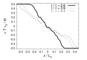
Figure 1: The horizontally ensemble-averaged temperature field at $t/\tau=2.6$ (solid line), $t/\tau=3.9$ (long-dashed line) and at $t/\tau=4.4$ (short-dashed line). The dimensional group $\tau\equiv(L_{z}/(Ag))^{1/2}$ is a characteristic time scale of the flow. Here, $A$ is the Atwood number, $g$ the gravitational acceleration and $L_{z}$ is the vertical size of the box. The value of $Ag$ is $0.15$.  Note the almost linear behaviour of $\langle T\rangle_{z}$ in the mixed layer.

It is worth noticing the almost linear behavior of the averaged temperature within the mixed layer. This is a first clue suggesting a possible relation between RT turbulence and the 2D Boussinesq driven convection studied in Refs. cmv01 ; cmmv02 . Further evidences will be given momentarily. In that particular instance of two-dimensional convection, turbulent fluctuations are driven by an external, linearly behaving with the elevation, temperature profile and the emergence of the Bolgiano regime clearly appears from data cmv01 . We will argue that 2D RT turbulence corresponds to the case driven by a linear temperature profile with a mean gradient that adiabatically decreases in time as $\Theta/L\sim t^{-2}$.
The mixing layer growth rate is shown in Fig. 2 in terms of the growth-rate parameter $\alpha$. Consistently with previous findings the mixing layer grows quadratically in time, i.e. $\alpha$ becomes almost constant in time nota1 , reaching the value $\alpha\sim 0.12$. The latter value is in agrement with the one found in Ref. clark (see the case $\chi=0.01$).

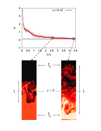
Figure 2: The time evolution of the layer-growth parameter $\alpha\equiv[(1/Ag)]dL/d(t^{2})$, $L$ being the mixing layer width. Heavy line represents the ensemble-averaged quantity while thin lines refer to each individual realization thus giving an indication of the level of fluctuations. The horizontal line refers to the value of $\alpha$ found in clark and it is shown for comparison. The mixing layer width $L(t)$ is defined as the distance between $z$-levels at which $\mathcal{F}\equiv(\langle T\rangle_{z}-T_{c})/(T_{h}-T_{c})=1\%$ and $99\%$, respectively. $T_{c}$ and $T_{h}$ are the temperature of the cold and hot fluid, before the mixing process takes place. Two snapshots of the temperature field are shown at $t/\tau=2.6$ (on the left) and at $t/\tau=4.4$ (on the right). Dark (white) areas identify cold (hot) regions.

In order to quantitatively assess the presence of Bolgiano’s regime for RT turbulence, let us focus on scaling behavior of stucture functions. For both velocity and temperature differences they are shown in Fig. 3. On the one hand, second-order structure functions follow the dimensional predictions (3) and (4). On the other hand, moments of order $4$ and $6$ display intermittency corrections for the temperature, e. g. deviations from (3), while this is not the case for the velocity which shows a close-to-Gaussian probability density function for inertial range increments (not shown).

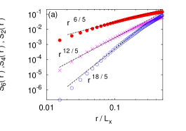
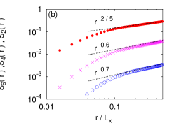
Figure 3: The moments of longitudinal velocity differences $S^{V}_{n}(r)$ (a) and temperature differences $S^{T}_{n}(r)$ (b). We consider the isotropic contribution to the statistics, by averaging over all directions of separations $\mathbf{r}$. In (a) dashed lines are the Bolgiano’s dimensional predictions, $S^{V}_{n}\sim r^{3n/5}$ bo59 . In (b), for $n=2$ the dashed line is the Bolgiano’s dimensional prediction: $S^{T}_{2}\sim r^{2/5}$ bo59 . For $n=4,6$ scaling exponents are anomalous, and their values are compatible with those of the $2D$ turbulent convection model of Refs. cmv01 ; cmmv02 (dashed lines). Moments are averaged over different $L$’s ranging from $L/L_{z}=0.4$ to $L/L_{z}=0.6$ (Fig. 4).

The slopes of Fig. 3 we have associated to $S_{4}^{T}$ and $S_{6}^{T}$ are relative to the scaling exponents found in Ref. cmv01 . This is a further quantitative evidence in favour of the equivalence between RT turbulence and Boussinesq turbulence in two dimensions cmv01 . With the present statistics, moments of order higher than $6$ are not accessible.

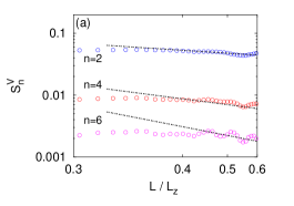
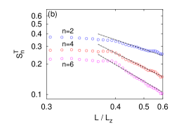
Figure 4: Evolution with $L$ of (a) moments of velocity differences $S^{V}_{n}$ and (b) temperature differences $S^{T}_{n}$. The results are obtained by averaging over a fixed range of separations belonging to the inertial scales. We found a better scaling behavior by displaying the behavior of structure functions as a function of the mixing layer width, $L$, rather than with respect to time. Those are connected by the relation $L\sim t^{2}$. The dash-dotted lines correspond to the dimensional scaling for velocity and to the intermittency-corrected scaling for temperature (see text for details).

We can further corroborate our claim on the possible equivalence between RT and driven 2D Boussinesq turbulence by looking at the temporal behavior of structure functions. Dimensional predictions immediately follow from Eqs. (3) and (4). The latter are well verified for all displayed orders for the velocity field (see Fig. 4). For the temperature field, anomalous corrections start to appear at the fourth order and are of the form $S_{n}^{T}(r)\sim\Theta^{n}(r/L(t))^{n/5}(r/L(t))^{-\sigma_{n}}$. If we assume (see Fig. 3) that the present RT model possesses the same spatial scaling exponents as those of the model presented in Ref. cmv01 , i.e. $S_{4}^{T}(r)\sim r^{0.6}$ and $S_{6}^{T}(r)\sim r^{0.7}$ (and thus $\sigma_{4}=0.2$ and $\sigma_{6}=0.5$), we immediately get a prediction for the exponents relative to the temporal behavior. We just have to remember that $L(t)\sim t^{2}$ to obtain the scaling relations $S_{4}\sim L^{-0.6}\sim t^{-1.2}$ and $S_{6}\sim L^{-0.7}\sim t^{-1.4}$. The latter are compatible with our results presented in Fig. 4 (b).

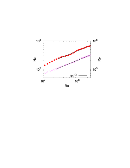
Figure 5: The behavior of the Nusselt number (bullets) and Reynolds number (circles) versus the Rayleigh number.

We end up by discussing the behavior of turbulent heat flux, mean temperature gradient and root-mean-square velocity as a function of time. These quantities are customarily represented in adimensional variables by the Nusselt number $Nu=[\langle v_{z}T\rangle L/(\kappa\Theta)]+1$, the Rayleigh number $Ra=g\beta\Theta L^{3}/(\nu\kappa)$ and the Reynolds number $Re=u_{rms}L/\nu$. The question about what functional relations exist among these quantities is a long-debated issue in the context of three-dimensional Rayleigh-Beńard turbulence (see, for example, Refs.S94 ; GL00 ; NSSD00 ; XBA00 ; NA03 and citations therein). In 2D RT turbulence exact expressions linking these adimensional numbers to temperature and kinetic energy input/dissipation rates can be derived closely following Ref. GL00 . For the RT case we have to deal with the additional complication of time-dependence yet compensated by the simplification originating from the absence of boundary effects. These relations read $\partial_{t}\langle{\bm{v}}^{2}/2\rangle=\nu\kappa^{2}L^{-4}(Nu-1)Ra-\epsilon_{v}$ and $\partial_{t}\langle\theta^{2}/2\rangle=\kappa\Theta^{2}L^{-2}(Nu-1)-\epsilon_{\theta}$, $\theta$ being the departure from the mean temperature profile. Since in 2D RT kinetic energy is transferred upscale we have a negligible $\epsilon_{v}$ and we can estimate a rate-of-change of kinetic energy $(\beta g\Theta)^{2}t$ from Eq. (4) and $L=\beta g\Theta t^{2}$. For the temperature we have $\langle\theta^{2}\rangle\sim\Theta^{2}$ independent of time. Temperature performs a direct cascade and thus dissipation can be estimated as $\delta_{L}\theta^{2}\delta_{L}v/L\sim\Theta^{2}/t$. Plugging those estimates into the exact relations yields $Nu\sim(\beta g\Theta)^{2}\kappa^{-1}t^{3}$ and $Ra\sim(\beta g\Theta)^{4}(\nu\kappa)^{-1}t^{6}$, therefore $Nu\sim Ra^{1/2}Pr^{1/2}$. As for the Reynolds number, Eq. (4) gives $Re\sim(\beta g\Theta)^{2}\nu^{-1}t^{3}\sim Ra^{1/2}Pr^{-1/2}$. It is worth remarking that a similar analysis for the 3D RT case leads mutatis mutandis to the same scaling laws. These, when considered as a function of $Ra$, coincide with the results derived by Kraichnan for the pure bulk contribution to 3D Rayleigh-Bénard turbulence. However, such Kraichnan scaling regime for RB convection, also dubbed “the ultimate state of thermal convection”, has so far eluded both experimental and numerical confirmation Amati2005 . Additionally, it has been shown that it is not realizable in the analytically tractable case of $Pr$ going to infinity Doering2005 . The reason may be traced back to the fundamental role played by the boundaries in establishing the turbulent heat transport in Rayleigh-Bénard convection. Indeed, when boundaries are artificially removed as in the numerical simulations of Refs. LT03 ; CLTT05 , the Kraichnan scaling is clearly observed. In this context, Rayleigh-Taylor turbulence provides a natural framework where heat transport takes place exclusively by bulk mechanisms and thus provides a physically realizable example of the Kraichnan scaling regime, inviting further experimental and numerical effort in this direction.

AM and LV have been supported by COFIN 2005 project n. 2005027808 and by CINFAI consortium. Simulations have been performed at CINECA (INFM parallel computing initiative). AC acknowledges the support of the European Union under the contract HPRN-CT-2002-00300 and PICS-CNRS 3057. Useful discussions with M. Chertkov are gratefully acknowledged.

References

- (1) Lord Rayleigh, Proc. London Math. Soc. 14, 170 (1883).
- (2) G.T. Taylor, Proc. R. London, Ser A 201, 192 (1950).
- (3) S.F. Gull, Royal Astronomical Society, Monthly Notices 171, 263, (1975).
- (4) M. Chertkov, Phys. Rev. Lett. 91, 115001 (2003).
- (5) A.N. Kolmogorov, Izv. Akad. Nauk SSSR, Ser. Fiz. VI, 56 (1941).
- (6) R. Bolgiano, J. Geophys. Res. 64, 2226 (1959).
- (7) T.T. Clark, Phys. Fluids 15, 2413 (2003).
- (8) R. H. Kraichnan and D. Montgomery, Rep. Prog. Phys. 43, 547 (1980).
- (9) P. Tabeling, Phys. Rep. 362, 1 (2002).
- (10) H. Kellay and W.I. Goldburg, Rep. Prog. Phys. 65, 845 (2002).
- (11) A. Celani, A. Mazzino, and M. Vergassola, Phys. Fluids 13, 2133 (2001).
- (12) A. Celani, T. Matsumoto, A. Mazzino, and M. Vergassola, Phys. Rev. Lett. 88, 054503 (2002).
- (13) We actually observe a slight decrease in time which has also been detected in Ref. clark and whose origin still remains a subject of discussions.
- (14) E.D. Siggia, Ann. Rev. Fluid. Mech. 26 137 (1994).
- (15) S. Grossmann and D. Lohse, J. Fluid Mech. 407, 27 (2000).
- (16) J. J. Niemela, L. Skrbek, K. R. Sreenivasan and R. J. Donnelly, Nature 404, 837 (2000).
- (17) X. Xu, K. M. S. Bajaj, and G. Ahlers, Phys. Rev. Lett. 84, 4357 (2000).
- (18) A. Nikolaenko and G. Ahlers, Phys. Rev. Lett. 91, 084501 (2003).
- (19) G. Amati, K. Koal, F. Massaioli, K. R. Sreenivasan and R. Verzicco, Phys. Fluids 17, 121701 (2005).
- (20) C. R. Doering, F. Otto, and M.G. Reznikoff J. Fluid Mech, submitted (2005).
- (21) D. Lohse, and F. Toschi, Phys. Rev. Lett. 90, 034502 (2003).
- (22) E. Calzavarini, D. Lohse, F. Toschi, and R. Tripiccione, Phys. Fluids 17, 055107 (2005).