Stability of a nonlinear oscillator with random damping

Abstract

A noisy damping parameter in the equation of motion of a nonlinear oscillator renders the fixed point of the system unstable when the amplitude of the noise is sufficiently large. However, the stability diagram of the system can not be predicted from the analysis of the moments of the linearized equation. In the case of a white noise, an exact formula for the Lyapunov exponent of the system is derived. We then calculate the critical damping for which the nonlinear system becomes unstable. We also characterize the intermittent structure of the bifurcated state above threshold and address the effect of temporal correlations of the noise by considering an Ornstein-Uhlenbeck noise.

1 Introduction

It is a well-known fact that a multiplicative noise acting on a dynamical system can generate unexpected phenomena such as stabilization Graham82b ; Lucke85 , stochastic transitions and patterns VandenBroeck94 or stochastic resonance Gammaitoni98 . As far as the stability of a random dynamical system is concerned, the exactly solvable example of a nonlinear first-order Langevin equation shows that the behaviour of the moments of the linearized equation can be misleading : higher moments seem to be always unstable although it is known that the critical value of the control parameter is the same as that of the deterministic system Graham82 . This apparent contradiction is due to the existence of long tails in the stationary probability distribution of the linearized equation which are suppressed when the nonlinearities are taken into account. The same type of conclusion can be drawn for a second-order system, namely a nonlinear oscillator with fluctuating frequency. The energetic stability analysis of the linearized system has been performed long ago Bourret71 ; Bourret73 but it leads to an erroneous phase diagram. In fact, because of the nonlinearities, the noise can even enhance the stable phase Graham82b ; Lucke85 . Besides, a non-perturbative reentrant transition can occur : a noise of small amplitude stabilizes the system, but a strong noise destabilizes it. Similar features hold in spatially extended systems such as the Ginzburg-Landau and Swift-Hohenberg equations driven by a noisy control parameter VandenBroeck94 ; Becker94 . Here again, the observed threshold shift can not be tackled by the analysis of the moments’ behaviour alone.

In this paper, we study the nonlinear oscillator with random damping. This dynamical system, in which the noise acts on the velocity variable rather than on the position, provides another example of a bifurcation induced by a multiplicative noise. This model was introduced in the study of the generation of water waves by wind West81 where the turbulent fluctuations in the air flow is modeled by a noise. This model is also relevant in the study of dynamical systems with an advective term where the corresponding velocity fluctuates. This problem has been investigated in VKampen74 ; Gitterman04 via the stability of the moments of the linearized equation. Here, we demonstrate that, as in the case of the random frequency oscillator, the moments stability analysis has no relevance and can not be used to derive the instability threshold. We shall obtain the exact phase diagram of the system thanks to an instability criterion valid for general nonlinear stochastic dynamical systems arnold ; Mallick03 .

The outline of this work is as follows. In section 2, we define the model and summarize the results obtained from the stability analysis of the moments. The main part of the paper (section 3) is devoted to the calculation of the Lyapunov exponent of the system from which the marginal stability curve is drawn. We then analyze the nature of the bifurcation and show that the bifurcated state is intermittent (section 4). In the last section, we consider an Ornstein-Uhlenbeck noise to investigate the effect of temporal correlations on the instability threshold.

2 Definition of the model and basic results

We consider the following stochastic dynamical system:

$$\ddot{x}+[r+ax^{2}-\xi(t)]\dot{x}+\alpha x=-bx^{3}\;,$$ (1)

where $\xi(t)$ is a white noise with intensity D and the parameters $a$ and $b$ are taken to be positive in order to have a stabilizing effect. The mean value of the damping $r$ is also positive whereas the coefficient $\alpha$ of the linear term can be either positive or negative. In fact, as far as the stability of the fixed point is concerned, the $\alpha<0$ case can be reduced to the $\alpha>0$ case as follows. For $\alpha<0$ and in the absence of noise, the oscillation around the $x=0$ position is unstable and the new equilibrium position in the saturated regime is $x_{0}=\pm\sqrt{-\alpha/b}$. Defining $y=x-x_{0}$, we observe that $y$ satisfies:

$$\ddot{y} + (r-\frac{a\alpha}{b}+2ax_{0}y+ay^{2})\dot{y}-2\alpha y$$

$$= \dot{x}\xi(t)-b(3x_{0}y^{2}-y^{3})\;.$$

The linear part of this equation is the same as that of equation (1) once the substitutions $r^{\prime}=r-a\alpha/b$ and $\alpha^{\prime}=-2\alpha$ are made. The coefficient $\alpha^{\prime}$ is now positive. We thus take $\alpha>0$. Before proceeding, we write time and position in dimensionless units by multiplying $t$ and $x$ by the factors $1/\sqrt{\alpha}$ and $\sqrt{a/r}$, respectively. Defining the following parameters:

$$\gamma=\frac{r}{\sqrt{\alpha}}\quad,\qquad\Delta=\frac{D}{\sqrt{\alpha}}\quad\text{and}\qquad k=\frac{br}{a\alpha}\;,$$ (3)

equation (1) becomes

$$\ddot{x}+\gamma(1+x^{2})\dot{x}+x=\dot{x}\xi(t)-kx^{3}\;,$$ (4)

where the autocorrelation of the white noise is given by $\langle\xi(t)\xi(t^{\prime})\rangle=\Delta\delta(t-t^{\prime})$ (as usual, the brackets represent an average on the realizations of the noise). The aim of this work is to study the stability of the fixed point $x=0$ of equation (4) as a function of the values of the different parameters $\gamma$, $\Delta$ and $k$.

We now summarize the results for the stability of the moments of the amplitude $x$, obtained by linearizing equation (4) around the fixed point $x=0$. It can be shown that the first moment satisfies :

$$\frac{d^{2}}{d\,t^{2}}\langle x\rangle+(\gamma-\frac{\Delta}{2})\frac{d}{d\,t}\langle x\rangle+\langle x\rangle=0\;.$$ (5)

The first moment remains bounded as $t\to\infty$ provided $\gamma>\Delta/2$. The effect of the noise is therefore to enhance the unstable phase. An intuitive argument of van Kampen VKampen74 explains why this should be the case : positive and negative fluctuations are equiprobable, but because the noise is multiplied by the velocity, the negative fluctuations have a stronger effect because they tend to increase the velocity (whereas the positive fluctuations decrease the velocity and have a lesser impact). For the second order moment, one must consider simultaneously $\langle x^{2}\rangle$, $\langle\dot{x}^{2}\rangle$ and $\langle x\dot{x}\rangle$, and study the linear system that couples them. These three quantities become zero in the long time limit provided $\gamma>\Delta$. In this case, the system is said to be ‘energetically’ stable. The instability threshold thus depends on the moment which is considered, due to the interplay between noise and nonlinearities. Therefore, in contrast to the deterministic case, a naive linear stability analysis fails to lead to conclusive results. A more refined criterion is needed to determine stability.

3 The Lyapunov exponent

The correct criterion that determines the stability of the fixed point $x=0$ is based upon the Lyapunov exponent $\Lambda$, defined as

$$\Lambda=\frac{1}{2}\langle\,\partial_{t}\ln[{\delta x}^{2}]\,\rangle=\langle\frac{\partial_{t}({\delta x})}{x}\,\rangle\,,$$ (6)

where ${\delta x}$ satisfies equation (4) linearized around $x=0$. It has been shown arnold ; Mallick03 ; Hansel89 that the sign of the Lyapunov exponent, calculated with the linear part of the equation, monitors the instability of the nonlinear oscillating system. When $\Lambda$ is negative, the trajectories of the nonlinear system (4) almost surely decay to zero and in the long time limit, the oscillator becomes localized in its rest position $x=0$. On the contrary, if $\Lambda>0$, the fixed point $x=0$ is unstable and the stationary probability density of the oscillator is extended.

We now calculate the Lyapunov exponent as a function of the parameters $\gamma$ and $\Delta$. Defining the variable $z$ as $z=\partial_{t}({\delta x})/{\delta x}$, the equation satisfied by $z$ is given by

$$\dot{z}=-1-\gamma z-z^{2}+z\xi(t)\;.$$ (7)

This is a Langevin equation involving the variable $z$ alone and coupled to a multiplicative noise (to be interpreted in the Stratonovich sense). By definition (6), we observe that

$$\Lambda(\gamma,\Delta)=\langle z\rangle\,.$$ (8)

Using standard techniques VKampen81 ; Gardiner84 , we obtain the Fokker-Planck equation for the probability density $P(z,t)$ at time $t$. The stationary probability density $P_{s}(z)$ satisfies:

$$\frac{\Delta}{2}\partial_{z}\bigl{[}zP_{s}(z)\bigr{]}+\frac{1+\gamma z+z^{2}}{z}P_{s}(z)=\frac{J}{z}\;,$$ (9)

where $J$ is the constant current of probability. Here, the current $J$ does not vanish; intuitively, this is due to the fact that $z$ plays the role of an angular variable in phase space and must be interpreted as a compact variable (see Risken for more details). Equation (9) can be solved by variation of constants method and we obtain

$$P_{s}(z)=\frac{2J}{\Delta} \int_{c}^{z} |\frac{t}{z}|^{1+2\gamma/\Delta}\frac{1}{t^{2}}\exp\Bigl{[}-\frac{2}{\Delta}\bigl{(}\Phi(z)-\Phi(t)\bigr{)}\Bigr{]}\,dt$$ (10)

$$+ A|z|^{-1-2\gamma/\Delta}\exp\Bigl{[}-\frac{2\Phi(z)}{\Delta}\Bigr{]}\;,$$

where $\Phi(t)=t-1/t$; the constant $A$ and the reference point $c$ are not determined at this stage. We must impose $A=0$ so that $P_{s}(z)$ is integrable at infinity (this implies $J\neq 0$). Furthermore, the function $\exp[\Phi(t)]$ is exponentially divergent when $t\to 0^{-}$; this remark fixes the choice of the value of $c$ in order to ensure that $P_{s}(z)$ is integrable at the origin (the cases $z<0$ and $z>0$ must be analyzed separately and two different reference points must be chosen). Finally, we obtain,

$$P_{s}(z)=\begin{cases}\frac{1}{N}\int_{-\infty}^{z}H(z,t)\,dt&\text{if}\quad z<0\\ \frac{1}{N}\int_{0}^{z}\;H(z,t)\,dt&\text{if}\quad z>0\\ \end{cases}$$ (11)

where $H(z,t)$ represents the function under the integral sign in (10). Using equation (9), we find that the probability density (11) satisfies

$$P_{s}(z) \sim \frac{J}{z^{2}}\quad\,\,\text{for}\,\,z\longrightarrow\pm\infty\,,$$ (12)

$$P_{s}(z) \sim J\qquad\text{for}\,\,z\longrightarrow 0\,.$$ (13)

This quadratic decay insures that the probability density is indeed normalizable at infinity. The normalization constant $N$ can calculated exactly gradstein and we obtain

$$N=\pi^{2}\Bigl{[}J_{2\gamma/\Delta}^{2}\bigl{(}\frac{4}{\Delta}\bigr{)}+Y_{2\gamma/\Delta}^{2}\bigl{(}\frac{4}{\Delta}\bigr{)}\Bigl{]}\;,$$ (14)

where $J$ and $Y$ are Bessel functions of the first kind and second kind, respectively. This formula was derived in Bouchaud87 for the study of diffusion in a random medium.

According to equation (8), the Lyapunov exponent is equal to the mean value of $z$ calculated with respect to $P_{s}(z)$; this quantity will be evaluated in the sense of principal parts

$$\Lambda=\lim_{M\rightarrow\infty}\int_{-M}^{+M}zP_{s}(z)dz\;.$$ (15)

(Thanks to equation (12), the logarithmic divergencies at $-\infty$ and $+\infty$ cancel with each other by parity). An exact closed formula for the Lyapunov exponent can then be derived and is given by

$$\Lambda=\frac{8}{N}\int_{0}^{+\infty}K_{1}\Bigl{(}\frac{8\sinh x}{\Delta}\Bigr{)}\sinh\Bigl{[}\bigl{(}1-\frac{4\gamma}{\Delta}\bigr{)}x\Bigr{]}\;dx\,,$$ (16)

where $K_{1}$ is a modified Bessel function of the second kind and the normalization constant $N$ is given in equation (14). From this expression, the instability threshold is readily found. Indeed, because the Bessel function is always positive, the sign of the Lyapunov is the same as that of the argument of the hyperbolic sine. We conclude that the fixed point $x=0$ is stable when

$$\gamma>\frac{\Delta}{4}\;.$$ (17)

We find, as usual, that the stable phase is wider than what moments stability predicts. Reverting to the initial variables, we observe that the instability threshold is given by $r=D/4$ which does not depend on the ‘linear frequency’ $\alpha$ of the oscillator. In the $(r,D)$ plane, the critical curve in the stability diagram of the $x=0$ fixed point is simply a straight line. We emphasize that this exact result is much simpler than that obtained for the Duffing oscillator with random frequency Mallick03 .

In figure 1, we plot the Lyapunov exponent of the nonlinear equation (4) for $\gamma=1$ and $\gamma=4$. We observe that, for $\Lambda<0$, the numerical findings and the analytical prediction are in perfect agreement. For higher values of the noise, the nonlinear term can not be neglected : whereas the linear Lyapunov exponent, given by equation (16) continues to grow, the Lyapunov exponent of the nonlinear equation saturates to a value close to 0. This indicates that the nonlinear system has gone through a bifurcation : the fixed point $x=0$ has become unstable and in the long time limit the system reaches an extended stationary state (in our case a noisy limit cycle). A remarkable feature of the curves displayed in figure 1, is that noise can have a stabilizing effect at small amplitudes : we notice that the curve for $\gamma=4$ decreases for small values of $\Delta$ and then increases. A closer inspection shows that this non-monotonic behaviour occurs when $\gamma>2$. This feature seems to contradict the argument, presented in section 2, stating that a noise in the damping term always has a distabilizing effect VKampen74 . This contradiction stems from the asymmetry of growth rate of the deterministic system around $\gamma=2$. Indeed, for $\gamma<2$ the growth rate is a linear function of $\gamma$ ($\sigma=-\gamma/2$), whereas it has a very different expression for $\gamma>2$ ($\sigma=-\gamma/2+\sqrt{\gamma^{2}-4}/2$). The positive and negative fluctuations of the growth rate are therefore intrinsically asymmetric, in contrast to the implicit assumption in van Kampen’s argument.

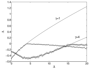
Figure 1: Typical evolution of the Lyapunov exponent as a function of the noise amplitude $\Delta$. The circles/crosses are obtained by numerical simulations of the nonlinear equation in the stationary regime for $\gamma=4$ and $\gamma=1$. The solid lines represent the theoretical values (16) for the linearized equation.

4 Intermittency above the threshold

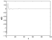
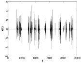
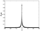
Figure 2: Numerical simulations of the system (4) with $\gamma=1$, $k=1$ and $\Delta=3$ (top left panel) corresponding to an absorbing state and for $\Delta=4.5$ (top right panel), corresponding to an intermittent state. The lower panels compares the probability distribution for $z$ obtained by simulations (dots) with the exact result (11) (full lines).

As shown in figure 2, the temporal series of the signal $x(t)$ exhibits “on-off intermittency”above the instability threshold (i.e., for a positive Lyapunov exponent). In other words, the amplitude $x$ is vanishingly small for the most of the time but exhibits sudden burst of activity. This behaviour has already been observed in chaotic systems Ott94 ; Sweet01 and in systems driven by multiplicative noise Japonais ; Japonais2 ; Tresser ; Leprovost05b ; Aumaitre05 . This intermittency can also be identified in the probability distribution density. In figure 3, we show the probability density of the energy of the oscillator defined as $r=\sqrt{x^{2}+\dot{x}^{2}}$. Near the origin, we observe that the probability distribution of $r$ is a power law which is generic of an intermittent signal. This power-law distribution for the energy of the oscillator can be derived as follows. From equation (4), we deduce that $r$ satisfies

$$\dot{r}=-(\gamma+\xi(t))r\sin^{2}\theta-\bigl{(}\gamma\sin^{2}\theta\cos^{2}\theta+k\cos^{3}\theta\sin\theta\bigr{)}r^{3}\;,$$

where $\theta=\arctan(\dot{x}/x)=\arctan(z)$. This equation, together with (7), forms a system of stochastic equations. A Fokker-Planck equation for the joint density $P(r,\theta)$ or $P(r,z)$ can be written but the resulting partial differential equation seems unlikely to be exactly solvable.

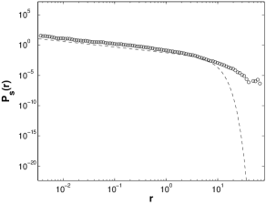
Figure 3: Probability density (in log-log scale) of the variable $r=\sqrt{x^{2}+\dot{x}^{2}}$ for $\gamma=1$, $\Delta=4.2$ and $k=1$. The dotted line corresponds to the approximation (18).

We therefore make an approximation along the lines of Mallick03 and assume that, for small values of $r$, the probability density is separable and can be written as $P(r,\theta)=P_{s}(r)P_{s}(\theta)$. An average over the angular variable yields an independent equation for $P_{s}(r)$ that can be exactly solved:

$$P_{s}(r)=\frac{1}{N_{r}}r^{(B/A)-1}\exp\Bigl{[}-\frac{Cr^{2}}{2A}\Bigr{]}\;,$$ (18)

where the coefficients $A,B$ and $C$ can all be expressed as mean values over the variable $z$ (or, equivalently, over the angular variable $\theta$) :

$$A=\langle\frac{\Delta\,z^{4}}{2(1+z^{2})^{2}}\rangle,\,B=\langle z^{2}\frac{\Delta-\gamma(1+z^{2})}{(1+z^{2})^{2}}\rangle,\,C=\langle\frac{\gamma z^{2}+kz}{(1+z^{2})^{2}}\rangle\,.$$

Multiplying equation (9) by $z^{2}/(1+z^{2})$ and integrating the result over $z$, the following identity is obtained :

$$B=\langle z\rangle=\Lambda\;.$$ (19)

The coefficient $A$ being a positive quantity, we remark that the function (18) is normalizable if and only if $B=\Lambda>0$. This provides a simple derivation of the stability criterion that we have used : when $\Lambda<0$, the fixed point $x=0$ is stable (the distribution (18) being not normalizable, the stationary distribution is the Dirac function at 0); when $\Lambda>0$, the fixed point is unstable and the stationary distribution is extended.

The distribution (18) is obviously a power law for small values of the variable $r$ which is an indication for intermittency. In figure 3, numerical results (open circles) for the probability distribution of the variable $r$ are compared with the analytical formula (18) (dashed line); the coefficients $A$, $B$ and $C$ have been calculated using (11). The agreement between the two curves is excellent as far as the power-law behaviour for small values of $r$ is concerned. For higher values of $r$, a discrepancy appears : the assumption that the stationary distribution is separable is no more valid and a specific analysis for large $r$ is needed Mallick03 . In figure 4, we plot the probability density of the energy for a greater value of the noise : again the small $r$ power law is very well described by equation (18).

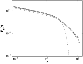
Figure 4: Probability density (in log-log scale) of the variable $r=\sqrt{x^{2}+\dot{x}^{2}}$ for $\gamma=1$, $\Delta=6$ and $k=1$.

5 Effect of a colored noise

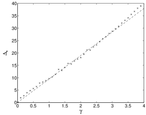
Figure 5: Critical amplitude $\Delta_{\star}$ of the noise versus $\gamma$ for a time correlation $\tau=1$. The dotted line is a linear fit.

In order to study the effect of the temporal correlations of the noise, we have performed numerical simulations of equation (4), taking the noise to be an Ornstein-Uhlenbeck process. In the stationary regime, the correlation of the Ornstein-Uhlenbeck process is exponential :

$$\langle\xi(t)\xi(t^{\prime})\rangle=\frac{\Delta}{2\tau}\exp\Bigl{[}-\frac{|t-t^{\prime}|}{\tau}\Bigr{]}\;.$$ (20)

Using the time series of the simulation results, we estimate the Lyapunov exponent (by computing $\langle\dot{x}/x\rangle$) and identify the bifurcation threshold. In figure 5, we plot the critical value of the noise intensity $\Delta$ for the onset of instability as a function of $\gamma$, the correlation time $\tau$ being equal to 1 (in dimensionless units). We observe that the critical curve has the shape of a straight line. Performing this analysis for different values of $\tau$, we have found that the critical amplitude $\Delta_{\star}$ of the noise is almost linear with $\gamma$; hence, to a good approximation, the critical curve is given by $\Delta_{*}(\gamma)=C(\tau)\gamma$. In figure 6, we plot $C(\tau)$ as a function of $\tau$; again the evolution is well described by a straight line in the range $0\leq\tau\leq 1$. These results indicate that the structure of the bifurcation diagram for the Ornstein-Uhlenbeck noise remains qualitatively the same as that for white noise.

Figure 6: Evolution of the critical slope as a function of the correlation time. The dotted line is a linear fit.

6 Conclusion

In this paper, we have studied the noise-induced bifurcation of a nonlinear oscillator with a fluctuating damping term. We have shown that the instability threshold of the nonlinear oscillator can not be determined from a stability analysis of the moments of the linearized problem; the system is indeed more stable than the analysis of moments indicates. This feature, that has already been noticed in a variety of models Graham82 ; Becker94 ; Mallick03 , can be explained by the existence of long tails in the probability distribution of the linearized system. These long tails have a greater influence on higher moments of $x$ which are therefore less and less stable. However, these long tails are suppressed for the nonlinear system, which has, therefore, a well defined stability threshold. For the problem considered here, an exact calculation of the Lyapunov exponent has allowed us to determine the exact stability diagram of the system. Besides, we have shown that a good quantitative description of the system in the vicinity of the bifurcation can be obtained if the probability distribution is assumed to be separable in energy and angle variables. This Ansatz allows us to calculate the power law exponent of the stationary probability and to predict intermittency. Our theoretical findings agree with numerical simulations. Finally, we have studied numerically the effect of temporal correlation of the noise by coupling our dynamical system to an Ornstein-Uhlenbeck process, and have found that the bifurcation scenario remains qualitatively the same. For this latter problem, exact analytical calculations seem to be out of reach; some quantitative information may, however, be obtained either by using one of the various Markovian approximations for colored noise, or by considering a special type of random process, such as the dichotomic Poisson noise which leads, in the present case, to an exactly solvable problem.

- (1) R. Graham, A. Schenzle, Phys. Rev. A 26, 1676 (1982)
- (2) M. Lücke, F. Schank, Phys. Rev. Lett. 54, 1465 (1985)
- (3) C.V. den Broeck, J.M.R. Parrondo, R. Toral, Phys. Rev. Lett. 73, 3395 (1985)
- (4) L. Gammaitoni, P. Hänggi, P. Jung, F. Marchesoni, Rev. Mod. Phys. 70, 223 (1998)
- (5) R. Graham, A. Schenzle, Phys. Rev. A 25, 1731 (1982)
- (6) R. Bourret, Physica 54, 623 (1971)
- (7) R. Bourret, U. Frisch, A. Pouquet, Physica 65, 303 (1973)
- (8) A. Becker, L. Kramer, Phys. Rev. Lett. 73, 955 (1994)
- (9) B.J. West, V. Seshadri, J. Geophys. Res. 86, 4293 (1981)
- (10) N.G. van Kampen, Physica 74, 239 (1974)
- (11) M. Gitterman, Phys. Rev. E 69, 41101 (2004)
- (12) L.Arnold, Random Dynamical Systems (Springer-Verlag, 1998)
- (13) K. Mallick, P. Marcq, Eur. Phys. J. B 36, 119 (2003)
- (14) D. Hansel, J.F. Luciani, J. Stat. Phys. 54, 971 (1985)
- (15) N.G. van Kampen, Stochastic processes in Physics and Chemistry (North-Holland, 1981)
- (16) C.W. Gardiner, Handbook of stochastic methods (Springer, 1984)
- (17) H. Risken, The Fokker-Planck equation (Springer, 1989)
- (18) I.S. Gradstein, I.M. Rhizik, Table of Integrals, Series and Products (Academic Press, 1994)
- (19) J.P. Bouchaud, A. Comtet, A. Georges, P. Ledoussal, Europhys. Lett. 3, 653 (1987)
- (20) E. Ott, J.C. Sommerer, Phys. Lett. A 188, 39 (1994)
- (21) D. Sweet, E. Ott, J.F. Finn, T.M. Antonsen, D.P. Lathrop, Phys. Rev. E 63, 66211 (2001)
- (22) T. Yamada, H. Fujisaka, Prog. Theor. Phys. 76, 582 (1986)
- (23) H. Fujisaka, H. Ishii, M. Inoue, T. Yamada, Prog. Theor. Phys. 76, 1198 (1986)
- (24) N. Platt, E.A. Spiegel, C. Tresser, Phys. Rev. Lett. 70, 279 (1993)
- (25) N. Leprovost, B. Dubrulle, Eur. Phys. J. B 44, 395 (2005)
- (26) S. Aumaître, F. Petrelis, K. Mallick, Phys. Rev. Lett. 95, 064101 (2005)